Crust and Upper Mantle Structure of Mars Determined from Surface Wave Analysis

Abstract

The crust and upper mantle structure of Mars is determined in the depth range of 0 to 100 km, by means of dispersion analysis and its inversion, which is performed for the surface waves present in the traces of the seismic event: S1094b. From these traces, Love and Rayleigh waves are measured in the period range of 4 to 40 s. This dispersion was calculated with a combination of digital filtering techniques, and later was inverted to obtain both models: isotropic (from 0 to 100 km depth) and anisotropic (from 0 to 15 km depth), which were calculated considering the hypothesis of the surface wave propagation in slightly anisotropic media. The seismic anisotropy determined from 0 to 5 km depth (7% of S-velocity variation and ξ ~ 1.1) could be associated with the presence of sediments or lava-flow layering, and wide damage zones surrounding the long-term fault networks. For greater depths, the observed anisotropy (17% of S-velocity variation and ξ ~ 1.4) could be due to the possible presence of volcanic materials and/or the layering of lava flows. Another cause for this anisotropy could be the presence of layered intrusions due to a single or multiple impacts, which could cause internal layering within the crust. Finally, the Moho depth is determined at 50 km as a gradual transition from crust to mantle S-velocities, through an intermediate value (3.90 km/s) determined from 50 to 60 km-depth.

1. Introduction

The knowledge of the Martian crust and upper mantle structure with depth is an important key to understanding its origin and evolution, but this structure remains among the least studied structures in geophysics and planetary science, due to the long distance of Mars from Earth, which has made the development and operation of scientific instruments in satellites and/or on land very difficult. However, in the last few years and with huge scientific and economic effort, the Interior Exploration Using Seismic Investigations, Geodesy, and Heat Transport (InSight) mission (which landed on Mars in Elysium Planitia) has provided the first seismic data recorded on the Martian surface. These invaluable seismic data have been analyzed to obtain the deep structure from P and S waves (e.g., [1]), the shallow structure from ambient-noise wavefield [2], and the crust and upper mantle structure from surface waves (e.g., [3]). The present study will complement the very scarce quantity of previous studies performed on the crust and upper mantle structure of Mars, with the dispersion analysis of the surface waves present in the record of the seismic event S1094b, and the inversion of this dispersion to calculate an S-velocity distribution with depth, for a depth range of 0 to 100 km, in which the seismic anisotropy present in the first 15 km of the crust will be considered. The seismic anisotropy in Mars has already been reported in previous studies [3,4,5], but only for the event S1222a. The seismic records obtained from InSight were analyzed by Kim et al. to obtain surface group velocities [3,6]. Unfortunately, most of these records do not present surface waves, because they are affected by strong contamination with long-period wind noise and atmospheric pressure waves, as well as a strong crustal scattering; only the records of three seismic events are suitable for surface wave analysis: S1000a, S1094b, and S1222a. The largest marsquake recorded during all InSight missions was S1222a, providing the first clear signals of surface waves and their first overtones [3]. On the other hand, S1000a provided unclear surface waves and only Rayleigh wave dispersion was determined by Kim et al. [6] due to its relatively small magnitude and large epicentral distance. The records of S1094b also were analyzed by Kim et al. [6], and they only determined Rayleigh wave dispersion. In the present study, the seismic anisotropy is reported for the first time for the event S1094b, and is also related, for the first time, to the possible presence of sediments or lava flow layering for the first 5 km depth, and volcanic materials from a 5 to 15 km depth.

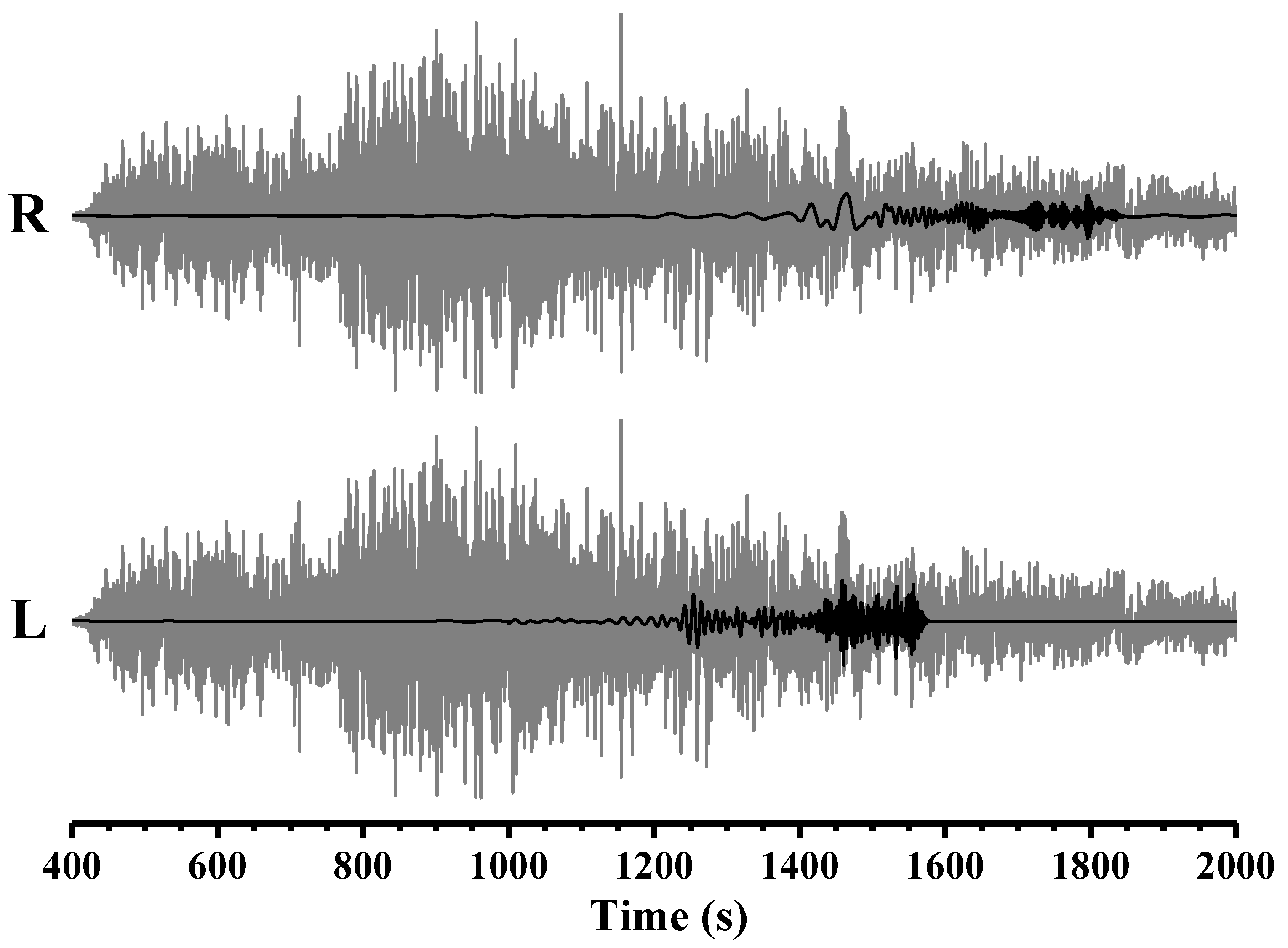
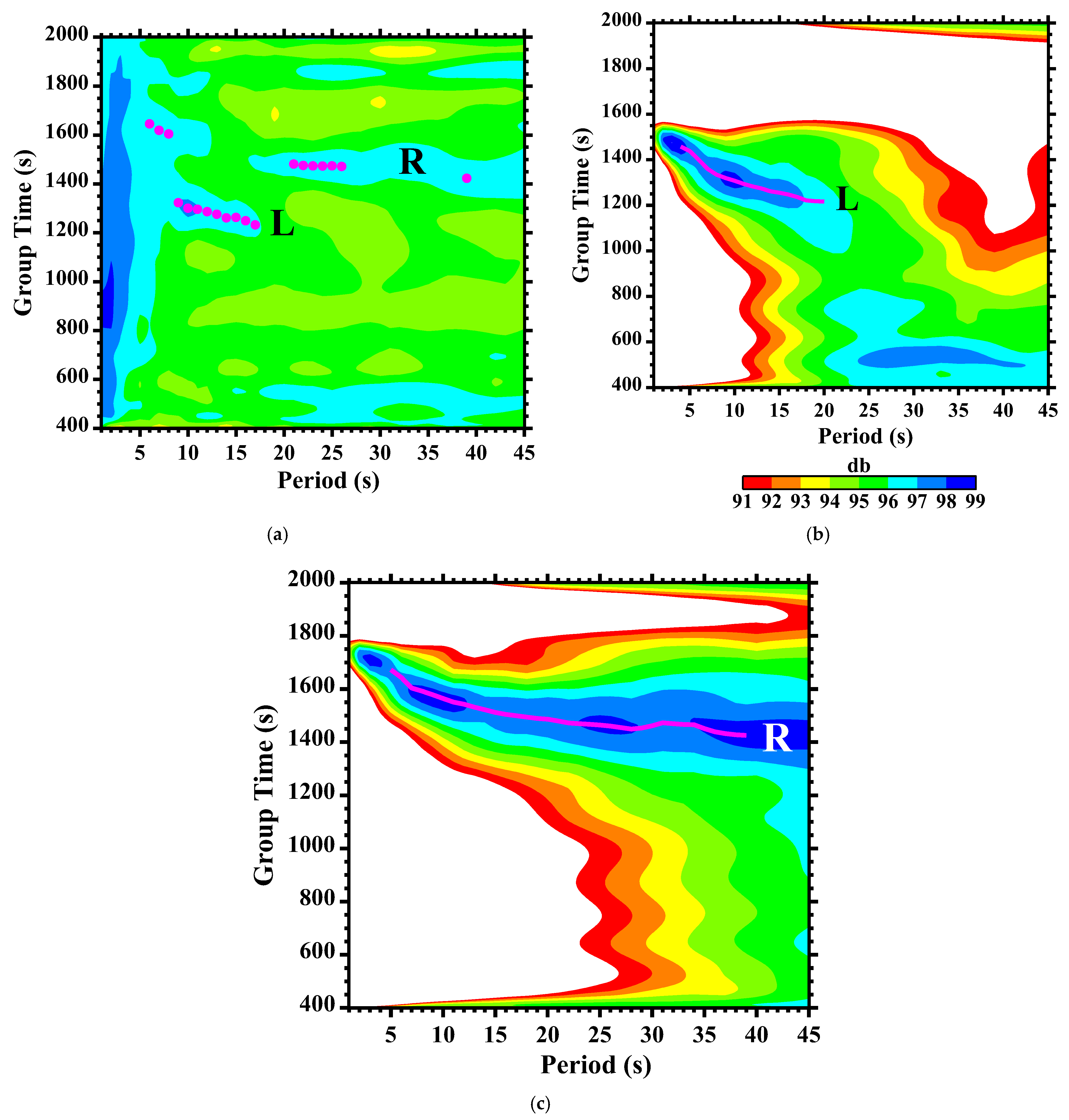
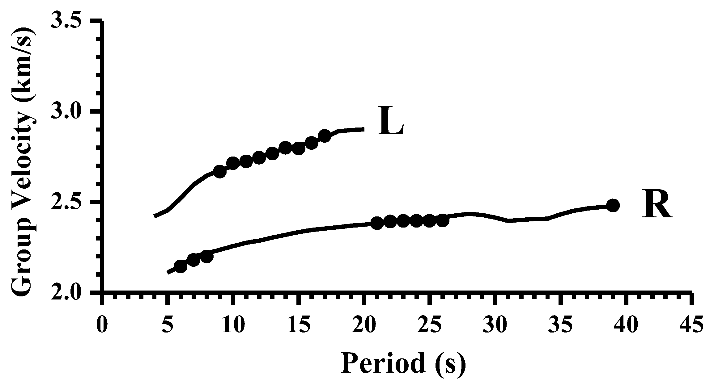
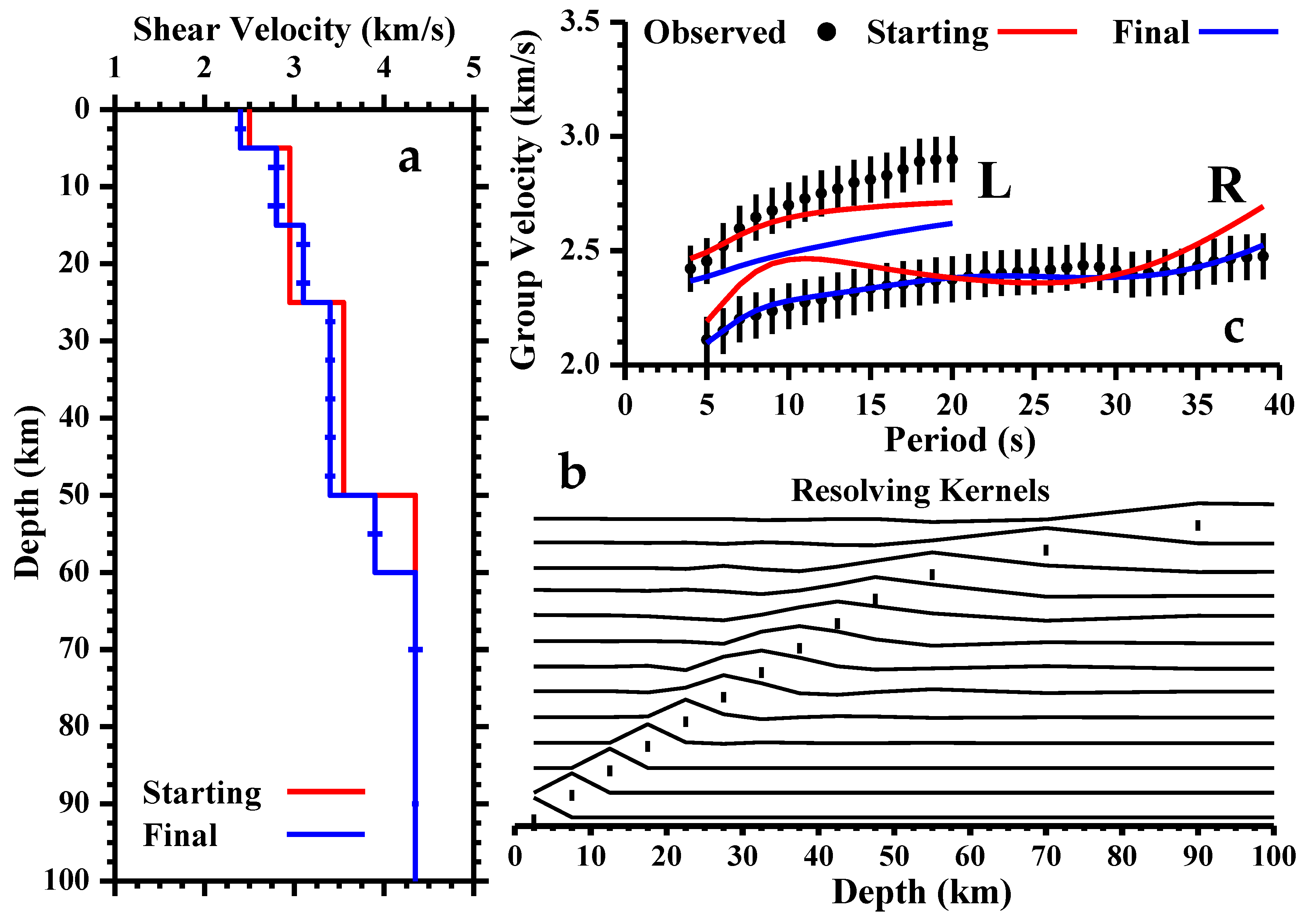
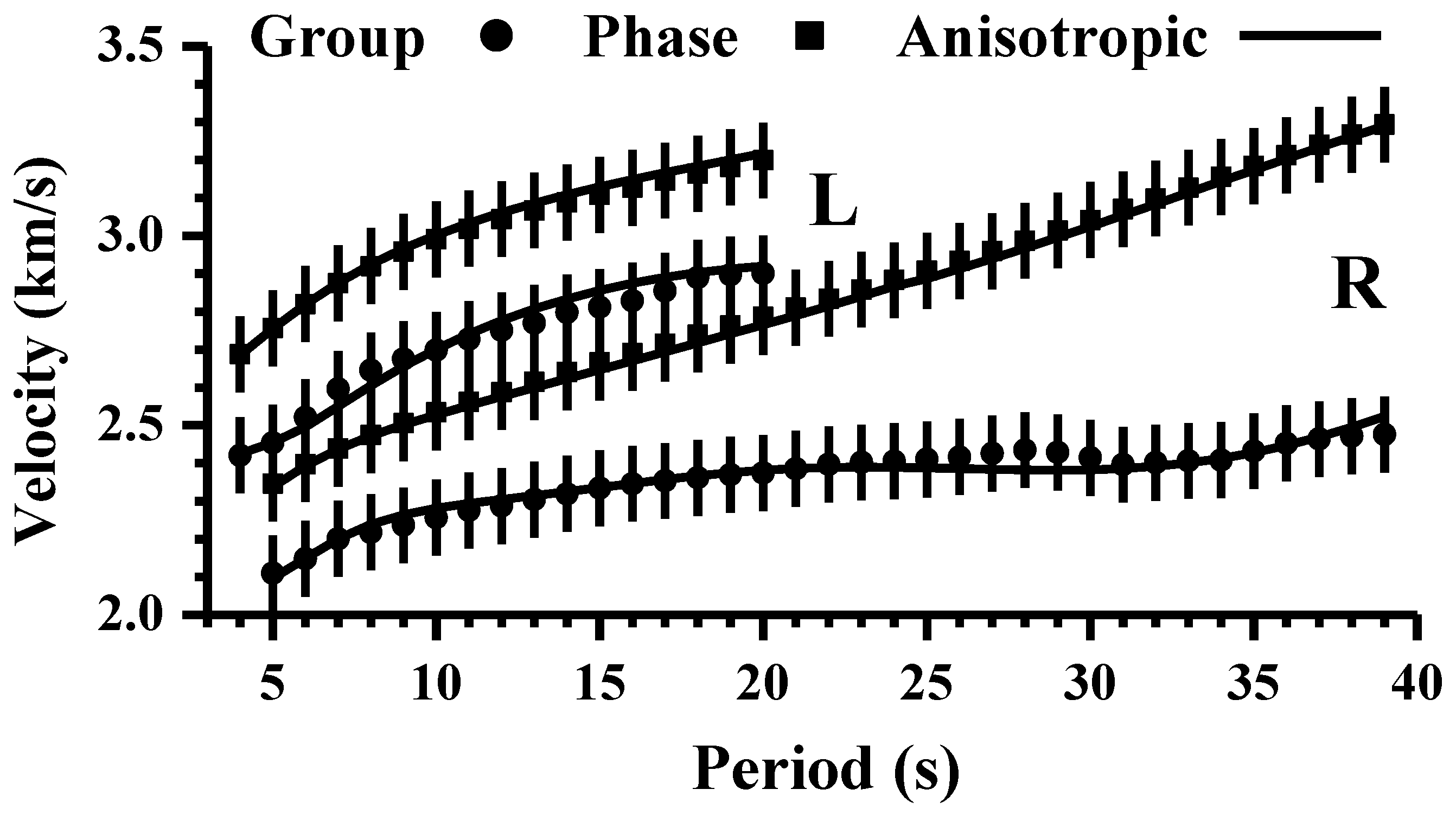
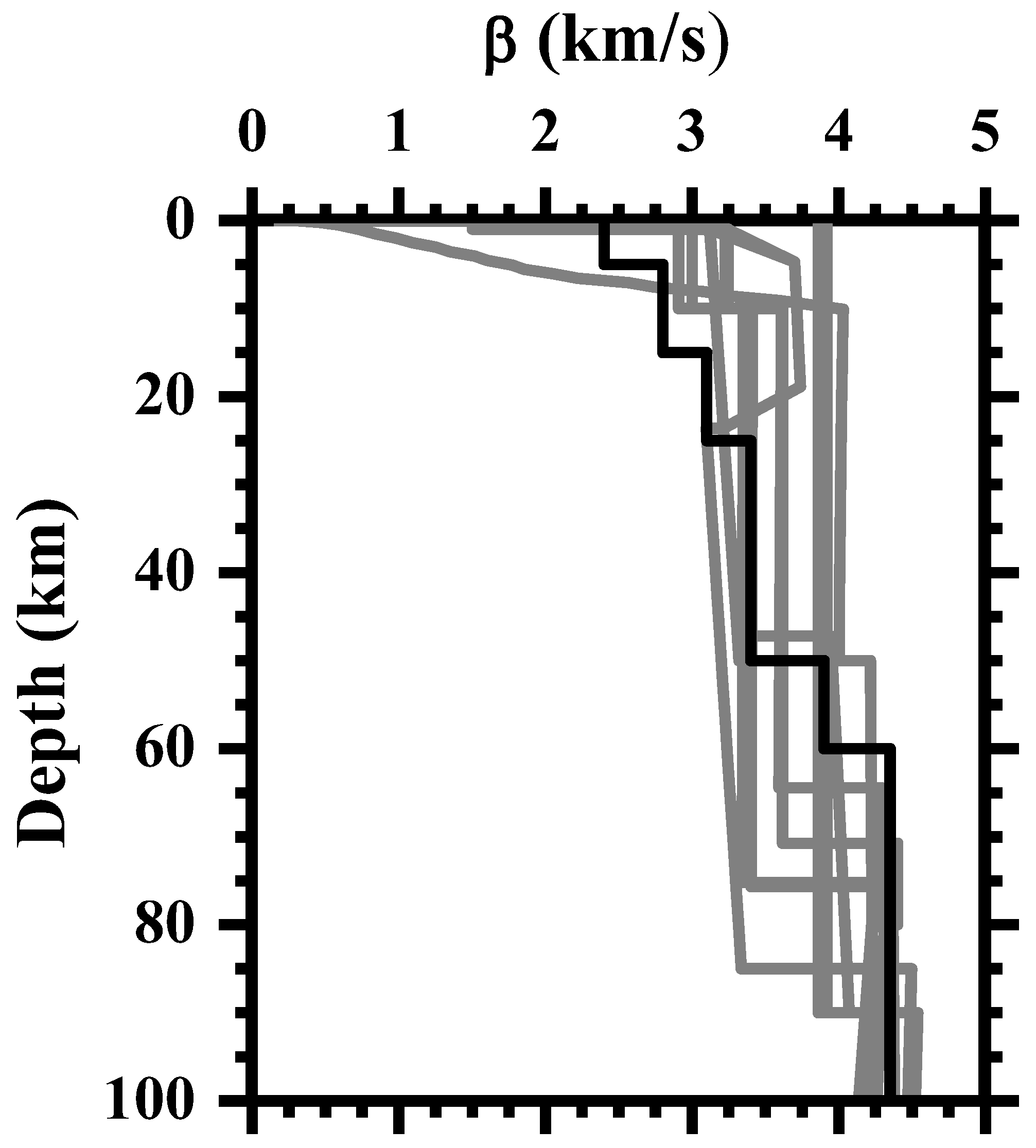
2. Data, Methodology, and Results

In the present study, the event S1094b (Supplement S1) recorded at the InSight seismic station (Supplement S2) has been revisited with the application of other filtering techniques [7], which have proven to be very useful techniques in several regions on Earth (e.g., [8]). This filtering analysis consists of a combination of the Multiple Filter Technique (MFT; [9]) and Time-Variable Filtering (TVF; [10]), as described by Corchete et al. [7], in which the MFT has been used to obtain the group-velocity dispersion curve from the time signals. The records of the vertical (Z), radial (R), and transverse (T) components of S1094b are obtained from its records in the three non-orthogonal components—UVW—of the seismic sensor [11], after instrument correction and removal of possible glitches [12]. Each of the ZRT records is a linear combination of all the UVW records, and all ZRT records have been analyzed in the present study, but the R and T records were discarded because they were affected by strong scattering. Thus, only the Z record (Figure 1, grey line) has been considered to determine the surface wave dispersion. Figure 2a (magenta points) and Figure 3 (black points) shows the initial group velocities calculated with the MFT, and applied to this record. TVF has been used to determine the smooth L- and R-signals shown in Figure 1 (black line), which are the time-variable filtered seismograms calculated from the original seismogram (Figure 1, grey line) and the initial group velocity (Figure 3, black points). Figure 3 (black line) shows the final group velocities calculated with the MFT (Figure 2b,c), applied to the L- and R-signals shown in Figure 1 (black line). The final dispersion curves for Love and Rayleigh waves shown in Figure 3 (black line) are considered as the observed data for the inversion process to be followed to calculate the S-velocity model, beneath the area crossed by the waves (Figure 4, [13]). The errors in the observed data are assumed as 0.1 km/s [7]. The initial model for this inversion process is listed in Supplement S3. This model has been prepared considering the previous models determined for the crust and mantle of Mars [3,6,14]. Figure 5 and Figure 6 show the inversion process for Love and Rayleigh waves, respectively [7]. The S-velocity models (Figure 5a and Figure 6a) and the resolving kernels (Figure 5b and Figure 6b) are plotted only for depths above 100 km, due to the poor resolution obtained for greater depths. The inversion process for Love wave dispersion gives an S-velocity model (Figure 5a), which is different to that calculated for the Rayleigh wave dispersion (Figure 6a), for the depth range of 0 to 15 km, i.e., the S-velocity model that satisfactorily fits the Love wave dispersion does not fit the Rayleigh wave dispersion (Figure 5c), and conversely, when the Rayleigh wave dispersion is properly fitted, the Love wave dispersion is not fitted (Figure 6c). The Love and Rayleigh wave dispersion are not compatible with a unique isotropic model (i.e., there is Love–Rayleigh discrepancy), and it is necessary to consider the existence of seismic anisotropy in the depth range of 0 to 15 km (Figure 5a and Figure 6a), defining an anisotropic model with hexagonal symmetry (i.e., azimuthal isotropy or transverse isotropy [15]). This model is calculated as described by Corchete [16]. In this methodology, the phase velocities are considered as observed data, and an isotropic model must be defined to calculate the anisotropic model, as a small perturbation of this isotropic model. In the present study, the Love and Rayleigh phase velocities (Figure 7, black rectangles) are calculated from the models shown in Figure 5a and Figure 6a by forward modelling [17,18], and it is selected as an isotropic model (Supplement S4) that is calculated from the inversion of the Rayleigh group velocities (Figure 6a). This methodology is improved in the present study considering the canonical harmonic components [19]: ${\mathrm{\gamma }}_{\mathrm{S}}^{00\mathrm{c}}$, ${\mathrm{\gamma }}_{\mathrm{A}}^{00\mathrm{c}}$, ${\mathrm{\gamma }}_{\mathrm{S}}^{20\mathrm{c}}$, ${\mathrm{\gamma }}_{\mathrm{A}}^{20\mathrm{c}}$ and ${\mathrm{\gamma }}_{\mathrm{S}}^{40\mathrm{c}}$, as linear functions of the P-velocities (α_H, α_V) and S-velocities (β_H, β_V), through to the perturbations γ_ijkl of the stiffness tensor [15,16,19]. Then, if a relation of $\mathrm{\alpha }=\sqrt{3}\mathrm{\beta }$ is assumed between the P- and S-velocities, the unknowns of the inverse problem can be reduced from 5 canonical harmonic components to 2 S-velocities, facilitating the fit of the observed data.

Table 1. S-velocities (β_H, β_V) calculated from the anisotropic inversion of the phase velocities shown in Figure 7 (black rectangles) for the first two layers of the isotropic model shown in Supplement S4. The P-velocities (α_H, α_V) are calculated as $\mathrm{\alpha }=\sqrt{3}\mathrm{\beta }$, and the parameters (ξ, φ) are calculated as defined by Babuska and Cara [15]. The S-velocity ratio (β_H − β_V)/β is given as a percentage, and β is given by Supplement S4.

Layer (n)	αH (km/s)	βH (km/s)	αV (km/s)	βV (km/s)	ξ (βH/βV)2	φ (αV/αH)2	$\frac{{\mathbf{\beta }}_{\mathbf{H}}-{\mathbf{\beta }}_{\mathbf{V}}}{\mathbf{\beta }}$
1	4.35 ± 0.12	2.51 ± 0.07	4.07 ± 0.14	2.35 ± 0.08	1.14	0.88	6.7
2	5.53 ± 0.16	3.19 ± 0.09	4.69 ± 0.14	2.71 ± 0.08	1.39	0.72	17.1

shows the results of this anisotropic inversion for the first two layers of Supplement S4 (from 0 to 15 km depth), and the values of the more frequently used quantities in anisotropic studies, as defined by Babuska and Cara [15]. The theoretical phase velocities calculated from this inversion are shown in Figure 7 (black lines), and their corresponding group velocities were computed by derivation [20]. Figure 7 shows the satisfactory fit obtained between the observed and theoretical dispersion curves, which was not possible with the isotropic inversion.

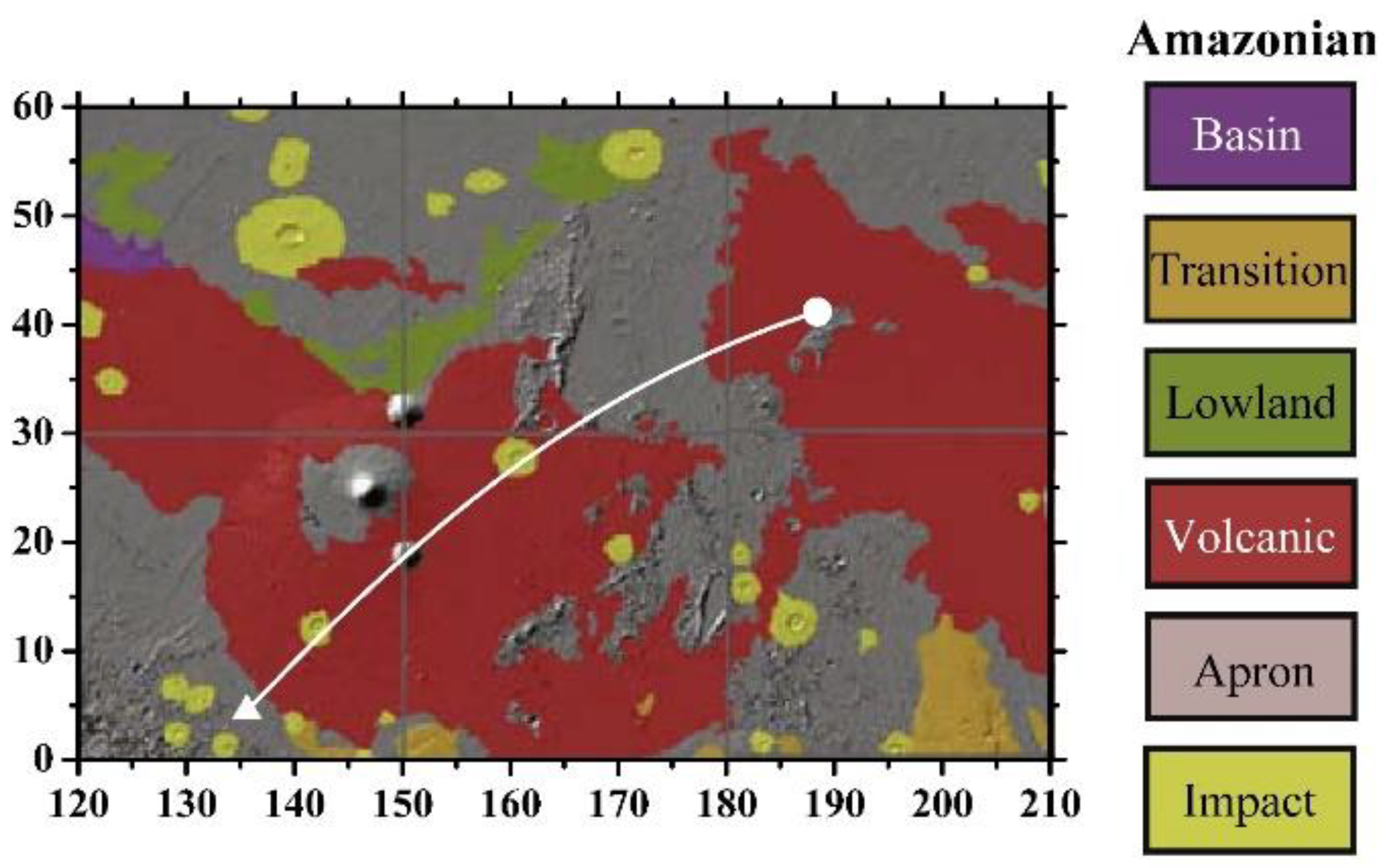
3. Interpretation and Discussion

Depth range: 0–5 km. There is a heterogeneous shallow crust that is constituted by several types of rocks, including sedimentary and igneous. This shallow crust is characterized by a wide range of densities and seismic velocities due to the presence of altered basalts, mudstones, shales, clays, sands, and loess, and it is expected to exhibit seismic anisotropy, as determined in the present study (7% of S-velocity variation for the layer 1 of Table 1), due to the presence of sediments or lava flow layering and wide damage zones surrounding the long-term fault networks [14].

Depth range: 5–15 km. The observed anisotropy at depths greater than 5 km is unlikely due to sedimentary layers, as in the previous depth range. For the present depth range, the presence of volcanic materials in the study area (Figure 4), such as andesite or altered basaltic rocks, could probably be the cause of the observed anisotropy (17% of S-velocity variation and ξ ~ 1.4 (layer 2 of Table 1)), which was also determined by Kim et al. [3] for another region of the Martian crust with 12% of S-velocity variation and ξ ~ 1.3. The layering of lava flows that could still exist for the present depth range could also be associated with this seismic anisotropy. Jiang et al. [21] have suggested that layered sill complexes can produce strong anisotropy (>8% S-velocity variation) at 5–18 km depth, but these complexes are usually very localized in depth and spatial extent, and are unlikely to be the cause of the observed anisotropy for this study area. Another cause for this anisotropy could be the presence of layered intrusions due to a single or multiple impacts [4]; such impacts could have caused internal layering within the crust, and the existence of seismic anisotropy.

Depth range: 15–100 km. In Figure 8, it is observed that all S-velocity models determined for Mars show similar values down to a 90 km depth, while these models show very different values up to this depth. This result is expected for Mars, because its Moho depth shows a great diversity of values from very shallow depths (< 10 km) to 90–100 km, depending on the region [14]: the northern lowlands show a uniformly thin crust (∼30 km thick), the southern highlands consist of a thick crust (∼60 km thick), and the Tharsis Rise (at the boundary between these two domains) is formed by a thick basaltic crust (∼100 km thick). For the study area (Figure 4), the Moho depth is determined at 50 km depth (Figure 8, black line), and this discontinuity is not sharp in terms of S-velocity, but a gradual transition from crust to mantle S-velocities, in which the S-velocity jumps from the crustal values (3.4 km/s) to mantle values (4.35 km/s) through an intermediate value (3.9 km/s) determined from 50 to 60 km depth. This Moho depth agrees well with that calculated in previous studies [6,22,23,24].

4. Conclusions

A dispersion analysis and its inversion is performed for the surface waves present in the record of the seismic event S1094b, and both models, isotropic (from 0 to 100 km depth) and anisotropic (from 0 to 15 km depth), are calculated considering the hypothesis of the surface wave propagation in slightly anisotropic media. From these models, the following conclusions are obtained:

Depth range: 0–5 km. The seismic anisotropy determined in the present study at this depth range (7% of S-velocity variation) could be associated with the presence of sediments or lava flow layering, and wide damage zones surrounding the long-term fault networks.

Depth range: 5–15 km. The observed anisotropy (17% of S-velocity variation and ξ ~ 1.4) at depths greater than 5 km could be due to the possible presence of volcanic materials in the study area, such as andesite or altered basaltic rocks. The layering of lava flows that still could exist for the present depth range of the study are, could also be associated with this seismic anisotropy. Another cause for this anisotropy could be the presence of layered intrusions due to a single or multiple impacts; such impacts could have caused internal layering within the crust and the existence of seismic anisotropy.

Depth range: 15–100 km. For Mars, the Moho depth shows a great diversity of values from very shallow depths (<10 km) to 90–100 km, depending on the region. For the present study area, the Moho depth is determined at 50 km, and this discontinuity is a gradual transition from crust to mantle S-velocities, in which the S-velocity jumps from the crustal values (3.4 km/s) to mantle values (4.35 km/s) through an intermediate value (3.90 km/s) determined from 50 to 60 km depth.

References

1. Khan, A.; Ceylan, S.; van Driel, M.; Giardini, D.; Lognonné, P.; Samuel, H.; Schmerr, N.C.; Stähler, S.C.; Duran, A.C.; Huang, Q.; et al. Upper mantle structure of Mars from InSight seismic data. Science 2021, 373, 434–438. [Google Scholar] [CrossRef] [PubMed]
2. Hobiger, M.; Halló, M.; Schmelzbach, C.; Stähler, S.C.; Fäh, D.; Giardini, D.; Golombek, G.; Clinton, J.; Dahmen, N.; Zenhäusern, G.; et al. The shallow structure of Mars at the InSight landing site from inversion of ambient vibration. Nat. Commun. 2021, 12, 6756. [Google Scholar] [CrossRef] [PubMed]
3. Kim, D.; Stähler, S.C.; Ceylan, S.; Lekic, V.; Maguire, R.; Zenhäusern, G.; Clinton, J.; Giardini, D.; Khan, A.; Panning, M.P.; et al. Structure along the martian dichotomy constrained by Rayleigh and love waves and their overtones. Geophys. Res. Lett. 2023, 50, e2022GL101666. [Google Scholar] [CrossRef]
4. Beghein, C.; Li, J.; Weidner, E.; Maguire, R.; Wookey, J.; Lekić, V.; Lognonné, P.; Banerdt, W. Crustal anisotropy in the Martian lowlands from surface waves. Geophys. Res. Lett. 2022, 49, e2022GL101508. [Google Scholar] [CrossRef]
5. Li, J.; Beghein, C.; Wookey, J.; Davis, P.; Lognonné, P.; Schimmel, M.; Stutzmann, E.; Golombek, M.; Montagner, J.-P.; Banerdt, W.B. Evidence for crustal seismic anisotropy at the InSight lander site. Earth Planet. Sci. Lett. 2022, 593, 117654. [Google Scholar] [CrossRef]
6. Kim, D.; Banerdt, W.B.; Ceylan, S.; Giardini, D.; Lekić, V.; Lognonné, P.; Beghein, C.; Beucler, É.; Carrasco, S.; Charalambous, C.; et al. Surface waves and crustal structure on Mars. Science 2022, 378, 417–421. [Google Scholar] [CrossRef]
7. Corchete, V.; Chourak, M.; Hussein, H.M. Shear wave velocity structure of the Sinai Peninsula from Rayleigh wave analysis. Surv. Geophys. 2007, 28, 299–324. [Google Scholar] [CrossRef]
8. Corchete, V. Crustal and upper-mantle structure beneath the South China Sea and Indonesia. Geol. Soc. Am. Bull. 2022, 133, 177–184. [Google Scholar] [CrossRef]
9. Dziewonski, A.; Bloch, S.; Landisman, M. A technique for the analysis of transient seismic signals. Bull. Seism. Soc. Am. 1969, 59, 427–444. [Google Scholar] [CrossRef]
10. Cara, M. Filtering dispersed wavetrains. Geophys. J. R. Astron. Soc. 1973, 33, 65–80. [Google Scholar] [CrossRef]
11. Lognonné, P.; Banerdt, W.B.; Giardini, D.; Pike, W.T.; Christensen, U.; Laudet, P.; de Raucourt, S.; Zweifel, P.; Calcutt, S.; Bierwirth, M.; et al. SEIS: Insight’s Seismic Experiment for Internal Structure of Mars. Space Sci. Rev. 2019, 215, 1–170. [Google Scholar] [CrossRef] [PubMed]
12. Scholz, J.R.; Widmer-Schnidrig, R.; Davis, P.; Lognonné, P.; Pinot, B.; Garcia, R.F.; Hurst, K.; Pou, L.; Nimmo, F.; Barkaoui, S.; et al. Detection, analysis, and removal of glitches from InSight’s seismic data from Mars. Earth Space Sci. 2020, 7, e2020EA001317. [Google Scholar] [CrossRef]
13. Tanaka, K.; Robbins, S.; Fortezzo, C.; Skinner, J.; Hare, T. The digital global geologic map of Mars: Chronostratigraphic ages, topographic and crater morphologic characteristics, and updated resurfacing history. Planet. Space Sci. 2014, 95, 11–24. [Google Scholar] [CrossRef]
14. Smrekar, S.E.; Lognonné, P.; Spohn, T.; Banerdt, W.B.; Breuer, D.; Christensen, U.; Dehant, V.; Drilleau, M.; Folkner, W.; Fuji, N.; et al. Pre-mission InSights on the Interior of Mars. Space Sci. Rev. 2019, 215, 3. [Google Scholar] [CrossRef]
15. Babuska, V.; Cara, M. Seismic Anisotropy in the Earth; Kluwer Academic: Dordrecht, The Netherlands, 1991. [Google Scholar]
16. Corchete, V. Review of the methodology for the inversion of surface-wave phase velocities in a slightly anisotropic medium. Comput. Geosci. 2012, 41, 56–63. [Google Scholar] [CrossRef]
17. Abo-Zena, A. Dispersion function computations for unlimited frequency values. Geophys. J. R. Astron. Soc. 1979, 58, 91–105. [Google Scholar] [CrossRef]
18. Aki, K.; Richards, P.G. Quantitative Seismology. In Theory and Methods; Freeman: San Francisco, CA, USA, 1980. [Google Scholar]
19. Smith, L.M.; Dahlen, F.A. The azimuthal dependence of Love and Rayleigh wave propagation in a slightly anisotropic medium. J. Geophys. Res. 1973, 78, 3321–3333. [Google Scholar] [CrossRef]
20. Ben-Menahem, A.; Singh, S.J. Seismic Waves and Sources; Springer: New York, NY, USA, 1981. [Google Scholar]
21. Jiang, C.; Schmandt, B.; Farrell, J.; Lin, F.-C.; Ward, K.M. Seismically anisotropic magma reservoirs underlying silicic calderas. Geology 2018, 46, 727–730. [Google Scholar] [CrossRef]
22. Zuber, M.T. The crust and mantle of Mars. Nature 2001, 412, 220–227. [Google Scholar] [CrossRef]
23. Neumann, G.A.; Zuber, M.T.; Wieczorek, M.A.; McGovern, P.J.; Lemoine, F.G.; Smith, D.E. Crustal structure of Mars from gravity and topography. J. Geophys. Res. 2004, 109, 08002. [Google Scholar] [CrossRef]
24. Bouley, S.; Keane, J.T.; Baratoux, D.; Langlais, B.; Matsuyama, I.; Costard, F.; Hewins, R.; Payré, V.; Sautter, V.; Séjourné, A.; et al. A thick crustal block revealed by reconstructions of early Mars highlands. Nat. Geosci. 2020, 13, 105–109. [Google Scholar] [CrossRef]
Figure 1. The Z-component seismogram (grey line) corresponding to S1094b (Supplement S1) recorded at Elyse (Supplement S2). The time-variable filtered seismograms (black line), corresponding to the Rayleigh (R) and Love (L) waves, were calculated from the observed seismogram (grey line) and the initial group velocities (Figure 3, black points).
Applsci 15 04732 g001
Figure 2. Contour maps of relative energy (normalized to 99 decibels) as a function of the period and the group time [7], calculated with the MFT applied to: (a) the observed seismogram (Figure 1, grey line); (b) the time-variable filtered seismogram corresponding to the Rayleigh wave dispersion (Figure 1, R-black line); (c) the time-variable filtered seismogram corresponding to the Love wave dispersion (Figure 1, L-black line). The magenta line and points denote the group times inferred from the energy map. The colour scale is the same for all maps. L and R denote Love and Rayleigh waves, respectively.
Applsci 15 04732 g002
Figure 3. The initial (black points) and the final (black line) group velocities calculated from the group times (Figure 2) and the epicentral distance [7]. L and R denote Love and Rayleigh waves, respectively.
Applsci 15 04732 g003
Figure 4. The path (white line), epicentre (white circle, Supplement S1), and station (white triangle, Supplement S2) plotted on the units present on Mars, grouped for the Amazonian period [13].
Applsci 15 04732 g004
Figure 5. (a) S-velocity (final model, blue line) obtained after the inversion process [7] of the Love wave dispersion curve (Figure 3, L-black line), and the initial model S-velocity (starting, red line) listed in Supplement S3. The horizontal bars show the standard deviation of S-velocity. (b) The resolving kernels of the inversion problem are posed. The reference depths, marked by vertical bars for the mean depth of each layer, are considered. (c) The theoretical Love and Rayleigh group velocity (blue line) calculated from the final model (a, blue line), and the theoretical Love and Rayleigh group velocity (red line) determined from the initial model (a, red line). The dots denote the Love and Rayleigh group velocities (Figure 3, black line), considered as observed data. The vertical bars show the error in group velocities at each period (1-σ errors).
Applsci 15 04732 g005
Figure 6. The same legend for (ac) as Figure 5, but now for Rayleigh wave.
Applsci 15 04732 g006
Figure 7. The phase velocities (black rectangles), considered as observed data for the anisotropic inverse problem, and their corresponding group velocities (black circles). The vertical bars show the standard deviation (1σ errors). The theoretical phase and group velocities, calculated from Supplement S4 and Table 1, are plotted with black lines. L and R denote Love and Rayleigh wave, respectively.
Applsci 15 04732 g007
Figure 8. A comparison between the S-velocity (β) listed in Supplement S4 (isotropic model) and that corresponding to several models determined prior to the InSight mission [14].
Applsci 15 04732 g008