

EL-MTSA: Stock Prediction Model Based on Ensemble Learning and Multimodal Time Series Analysis


Abstract
1. Introduction
- We propose a novel integrated approach to enhance the robustness of predictions. By applying discrete wavelet transform to data with different sampling frequencies, we effectively reduce noise and minimize correlations within the data. Additionally, the use of a variational autoencoder for sentiment data enables efficient and meaningful encoding, further improving the model’s performance.
- We incorporate news sentiment indicators into the dataset using a multimodal approach, promoting the interaction between external demand and cognitive inner demand to enhance data complementarity in predictions.
- We introduce a new method for processing high-frequency time series data, enabling the simultaneous representation of intra-cycle and intra-week variations.
- We employ Bayesian optimization to automate parameter selection and improve network efficiency.
2. Related Work
2.1. Traditional Stock Prediction Models
2.2. Sentiment Information and Stock Forecasting
2.3. Applications of Ensemble Learning Models
3. Model Construction
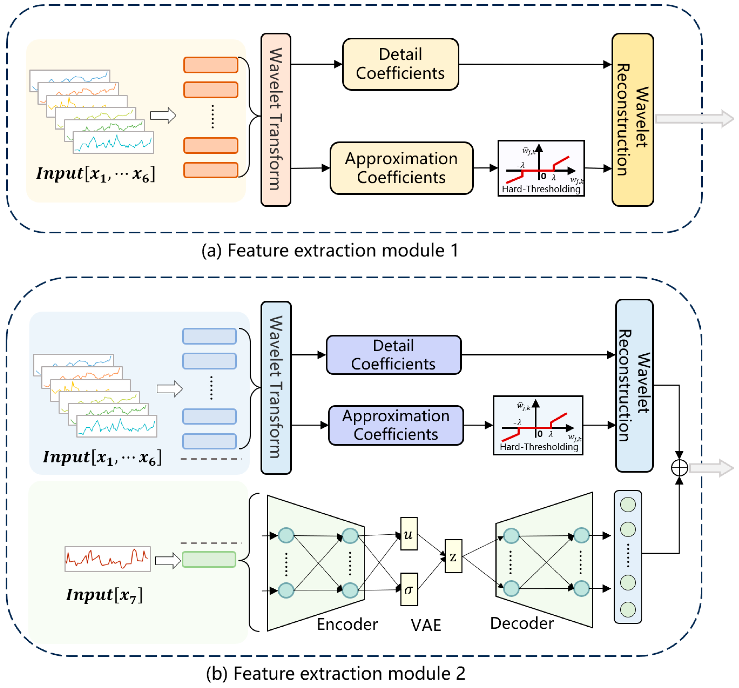
3.1. Feature Extraction Module
3.2. Deep-Learning-Based Sequential Prediction Network
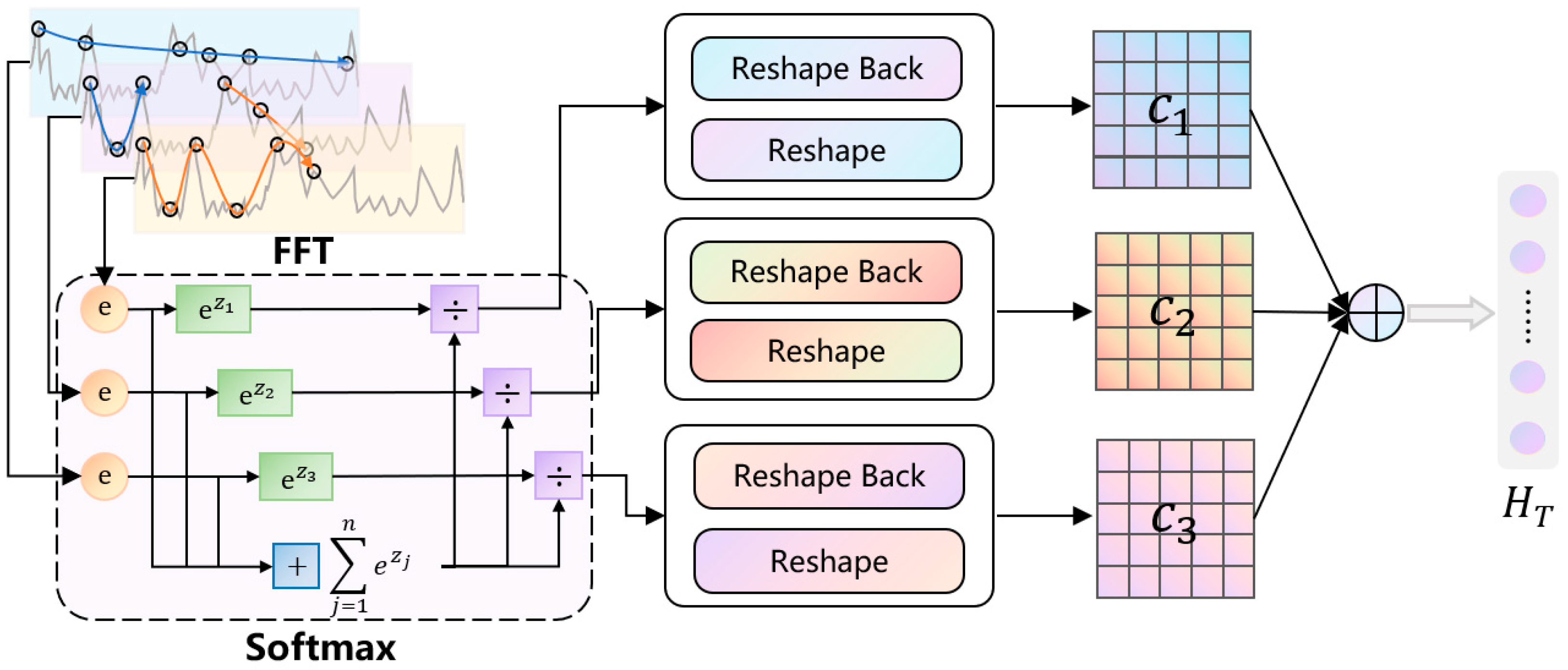
3.3. Learning Optimization Module via Information Fusion Strategy
3.4. Hyperparameter Optimization Based on Bayesian Inference
4. Experimental Results and Discussion
4.1. Data Sources
4.2. Training Parameter Setting
4.3. Evaluation Metrics
4.4. Experimental Results and Analyses
4.4.1. Reliability Analyses of Sentiment Indicators
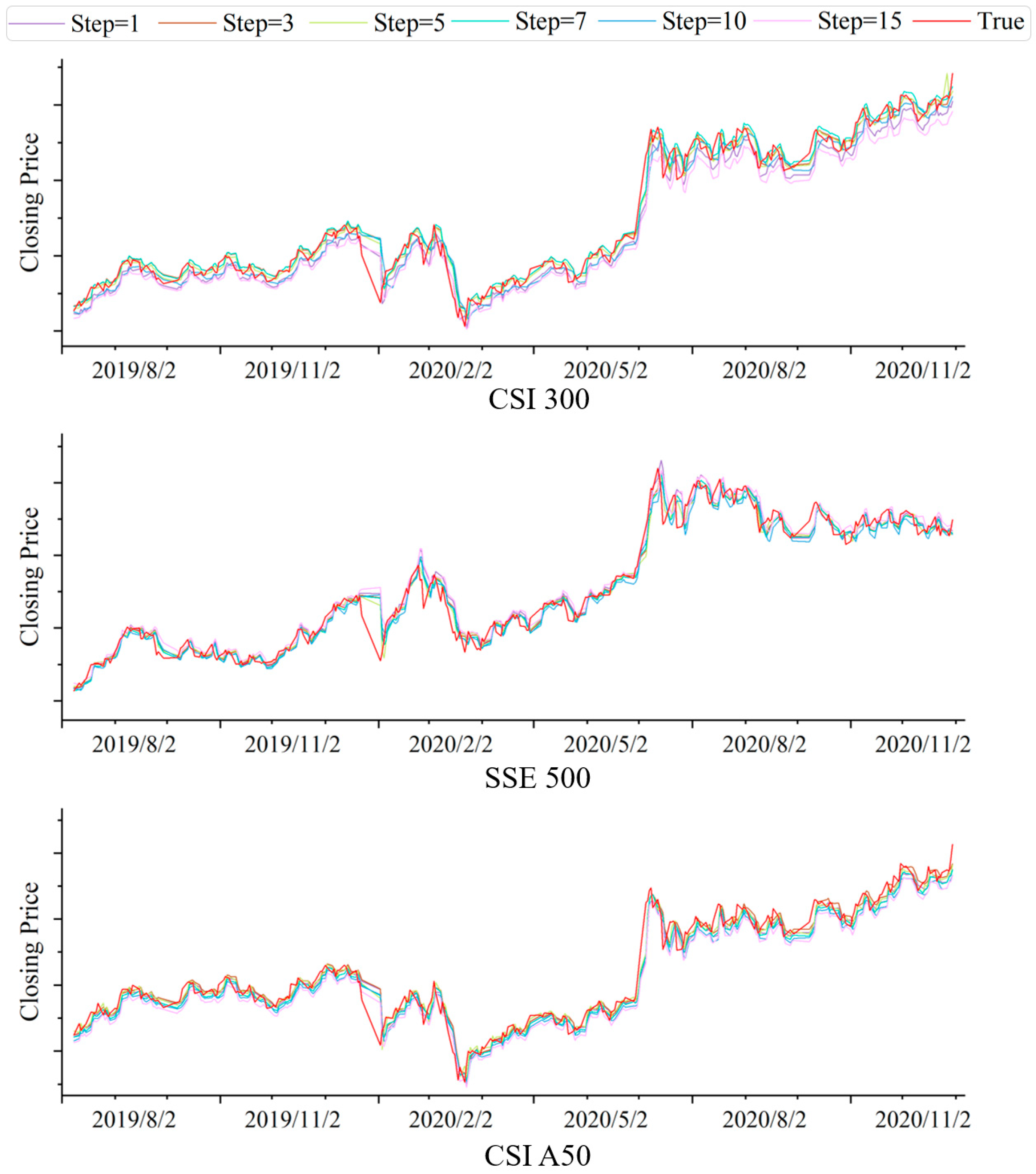
4.4.2. Prediction Results for Different Window Steps
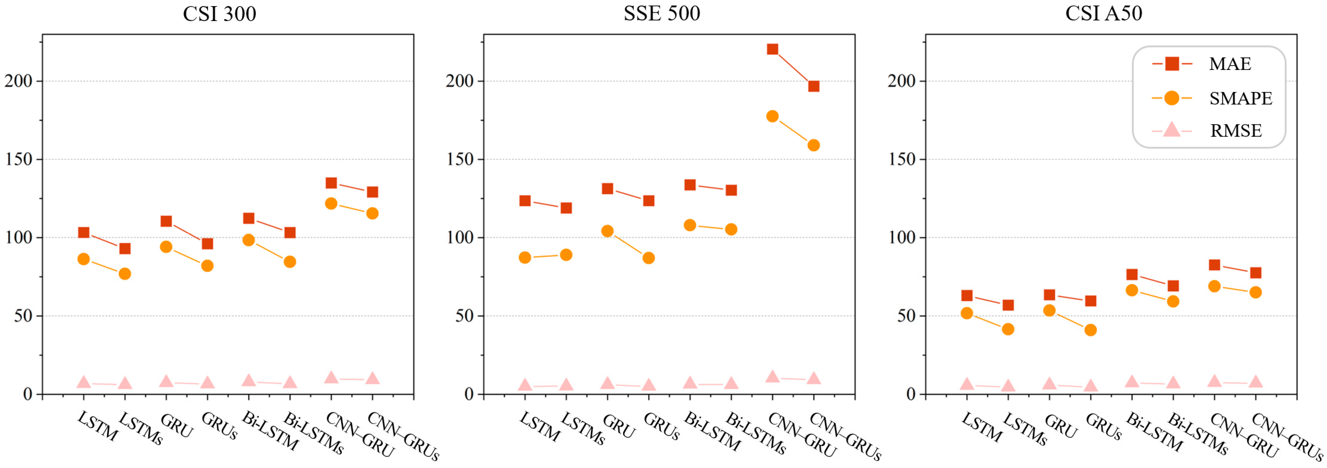
4.4.3. Ablation Experiment Results and Analysis
4.4.4. Comparative Analysis of Data Volume
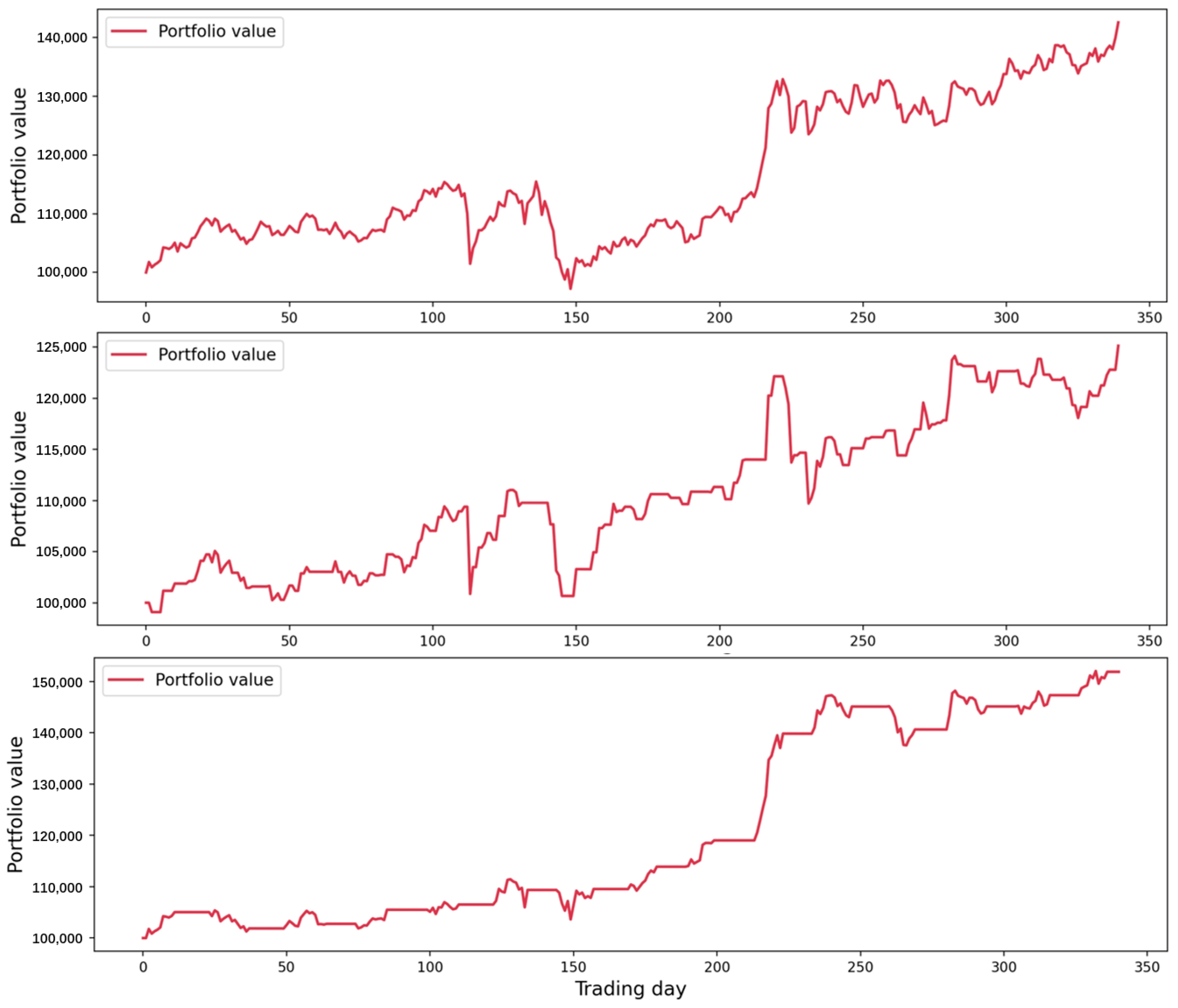
4.4.5. Comparative Analysis of Simulated Investments
- (1)
- Final portfolio value (FPV) is the total value of the investment portfolio at the end of the simulation period, reflecting the cumulative growth of the initial capital.
- (2)
- Total profit (TP) is the absolute monetary gain achieved over the investment horizon, calculated as the difference between the final portfolio value and the initial capital.
- (3)
- Maximum drawdown (MDD) is the largest peak-to-trough decline in portfolio value during the simulation period, expressed as a percentage of the peak value. This metric quantifies the worst-case loss and serves as a critical measure of downside risk.
- (4)
- Sharpe ratio (SR) is a risk-adjusted performance measure that evaluates the excess return per unit of risk, with risk represented by the standard deviation of portfolio returns. This metric provides insights into the efficiency of returns relative to the level of risk undertaken.
4.4.6. Cross-Market-Cycle Generalization Capability Assessment
4.5. Discussion
5. Conclusions
Author Contributions
Funding
Institutional Review Board Statement
Informed Consent Statement
Data Availability Statement
Conflicts of Interest
References
- Liu, X.; Guo, J.; Wang, H.; Zhang, F. Prediction of Stock Market Index Based on ISSA-BP Neural Network. Expert Syst. Appl. 2022, 204, 117604. [Google Scholar] [CrossRef]
- Debnath, P.; Srivastava, H.M. Optimizing Stock Market Returns During Global Pandemic Using Regression in the Context of Indian Stock Market. Risk Financ. Manag. 2021, 14, 386. [Google Scholar] [CrossRef]
- Fama, E.F. Efficient Capital Markets: A Review of Theory and Empirical Work. J. Financ. 1970, 25, 383–417. [Google Scholar] [CrossRef]
- Lv, P.; Shu, Y.; Xu, J.; Wu, Q. Modal Decomposition-Based Hybrid Model for Stock Index Prediction. Expert Syst. Appl. 2022, 202, 117252. [Google Scholar] [CrossRef]
- Weng, B.; Ahmed, M.A.; Megahed, F.M. Stock Market One-Day Ahead Movement Prediction Using Disparate Data Sources. Expert Syst. Appl. 2017, 79, 153–163. [Google Scholar] [CrossRef]
- Ballings, M.; Van den Poel, D.; Hespeels, N.; Gryp, R. Evaluating Multiple Classifiers for Stock Price Direction Prediction. Expert Syst. Appl. 2015, 42, 7046–7056. [Google Scholar] [CrossRef]
- Akyüz, A.O.; Uysal, M.; Bulbul, B.A.; Uysal, M.O. Ensemble Approach for Time Series Analysis in Demand Forecasting: Ensemble Learning. In Proceedings of the 2017 IEEE International Conference on Innovations in Intelligent Systems and Applications, Gdynia, Poland, 3–5 July 2017; pp. 7–12. [Google Scholar]
- Bergquist, S.L.; Brooks, G.A.; Keating, N.L.; Landrum, M.B.; Rose, S. Classifying Lung Cancer Severity with Ensemble Machine Learning in Health Care Claims Data. In Proceedings of the 2nd Machine Learning for Healthcare Conference, Boston, MA, USA, 18–19 August 2017; pp. 25–38. [Google Scholar]
- Priya, P.; Muthaiah, U.; Balamurugan, M. Predicting Yield of the Crop Using Machine Learning Algorithm. Int. Eng. Sci. Res. Technol. 2018, 7, 1–7. [Google Scholar]
- Khairalla, M.A.; Ning, X.; Al-Jallad, N.T.; El-Faroug, M.O. Short-Term Forecasting for Energy Consumption through Stacking Heterogeneous Ensemble Learning Model. Energies 2018, 11, 1605. [Google Scholar] [CrossRef]
- Zhao, Y.; Li, J.; Yu, L. A Deep Learning Ensemble Approach for Crude Oil Price Forecasting. Energy Econ. 2017, 66, 9–16. [Google Scholar] [CrossRef]
- Macchiarulo, A. Predicting and Beating the Stock Market with Machine Learning and Technical Analysis. Intern. Bank. Commer. 2018, 23, 1–22. [Google Scholar]
- Wu, S.; Liu, Y.; Zou, Z.; Weng, T.-H. S_I_LSTM: Stock Price Prediction Based on Multiple Data Sources and Sentiment Analysis. Connect. Sci. 2021, 34, 44–62. [Google Scholar] [CrossRef]
- Porshnev, A.; Redkin, I.; Shevchenko, A. Machine Learning in Prediction of Stock Market Indicators Based on Historical Data and Data from Twitter Sentiment Analysis. In Proceedings of the IEEE International Conference on Data Mining Workshops, Shenzhen, China, 14 December 2014. [Google Scholar]
- Matías, J.M.; Reboredo, J.C. Forecasting Performance of Nonlinear Models for Intraday Stock Returns. J. Forecast. 2012, 31, 172–188. [Google Scholar] [CrossRef]
- Challa, M.L.; Malepati, V.; Kolusu, S.N.R. S&P BSE Sensex and S&P BSE IT Return Forecasting Using ARIMA. Financ. Innov. 2020, 6, 47. [Google Scholar]
- Arnerić, J.; Poklepović, T. Nonlinear Extension of Asymmetric GARCH Model within Neural Network Framework. Comput. Sci. Inf. Technol. 2016, 6, 101–111. [Google Scholar]
- Sangeetha, J.M.; Alfia, K.J. Financial Stock Market Forecast Using Evaluated Linear Regression Based Machine Learning Technique. Meas. Sens. 2024, 31, 10095. [Google Scholar] [CrossRef]
- Santoso, M.; Sutjiadi, R.; Lim, R. Indonesian Stock Prediction Using Support Vector Machine (SVM). In Proceedings of the MATEC Web of Conferences, Bandung, Indonesia, 18 April 2018; p. 164. [Google Scholar]
- Loke, K.S. Impact of Financial Ratios and Technical Analysis on Stock Price Prediction Using Random Forests. In Proceedings of the IConDA, Kuching, Malaysia, 9–11 November 2017; pp. 38–42. [Google Scholar]
- Shih, C.M.; Yang, K.C.; Chao, W.P. Predicting Stock Price Using Random Forest Algorithm and Support Vector Machines Algorithm. In Proceedings of the IEEM, Singapore, 18–21 December 2023; pp. 133–137. [Google Scholar]
- Nelson, D.M.Q.; Pereira, A.C.M.; de Oliveira, R.A. Stock Market’s Price Movement Prediction with LSTM Neural Networks. In Proceedings of the IJCNN, Anchorage, AK, USA, 14–19 May 2017; pp. 1419–1426. [Google Scholar]
- Narayana, S.; Sri, S.N.D.; Kumar, S.R.; Ajay, T.; Vasiq, S.S. Predicting the Stock Market Index Using GRU for the Year 2020. In Proceedings of the ESIC, Bhubaneswar, India, 1 September 2024; pp. 399–404. [Google Scholar]
- Wu, J.M.-T.; Li, Z.; Srivastava, G.; Frnda, J.; Diaz, V.G.; Lin, J.C.-W. A CNN-Based Stock Price Trend Prediction with Futures and Historical Price. In Proceedings of the ICPAI, Taipei, Taiwan, 3–5 December 2020; pp. 134–139. [Google Scholar]
- Nikhil, S.; Sah, R.K.; Parki, S.K.; Tamang, T.B.; TR, M. Stock Market Prediction Using Genetic Algorithm Assisted LSTM-CNN Hybrid Model. In Proceedings of the ICCCNT, Delhi, India, 6–8 July 2023; pp. 1–6. [Google Scholar]
- Sulistio, B.; Warnars, H.L.H.S.; Gaol, F.L.; Soewito, B. Energy Sector Stock Price Prediction Using the CNN, GRU & LSTM Hybrid Algorithm. In Proceedings of the ICCoSITE 2023, Jakarta, Indonesia, 16–17 February 2023; pp. 178–182. [Google Scholar]
- Zheng, X.; Cai, J.; Zhang, G. Stock Trend Prediction Based on ARIMA-LightGBM Hybrid Model. In Proceedings of the ICTC, Nanjing, China, 6–8 May 2022; pp. 227–231. [Google Scholar]
- Chi, L.; Zhuang, X.; Song, D. Investor sentiment in the Chinese stock market: An empirical analysis. Appl. Econ. Lett. 2012, 19, 345–348. [Google Scholar] [CrossRef]
- Bouktif, S.; Fiaz, A.; Awad, M. Augmented Textual Features-Based Stock Market Prediction. IEEE Access 2020, 8, 40269–40282. [Google Scholar] [CrossRef]
- Shah, D.; Isah, H.; Zulkernine, F. Predicting the Effects of News Sentiments on the Stock Market. In Proceedings of the IEEE International Conference on Big Data (Big Data), Seattle, WA, USA, 10–13 December 2018. [Google Scholar]
- Bharti, S.K.; Tratiya, P.; Gupta, R.K. Stock Market Price Prediction Through News Sentiment Analysis & Ensemble Learning. In Proceedings of the iSSSC, Gunupur, India, 6–8 November 2022; pp. 1–5. [Google Scholar]
- Parashar, D.; D’Silva, M.; Kulshreshtha, S. A Machine Learning Framework for Stock Prediction Using Sentiment Analysis. In Proceedings of the GCAT, Bangalore, India, 6–8 December 2023; pp. 1–5. [Google Scholar]
- Cui, H.; Zhu, Y.; Gu, F.; Wang, L. Research on Stock Price Prediction Using TextRank-Based Text Summarization Technology and Sentiment Analysis. In Proceedings of the 2022 CIS, Chengdu, China, 16–18 December 2022; pp. 302–306. [Google Scholar]
- Kiran, S.; Dhana Lakshmi, P.; Sultana, N.; Naga Rama Devi, G.; Gothane, S.; Reddy Madhavi, K. Stock Market Price Prediction Using Sentiment Analysis. In Proceedings of the ICMEET, Singapore, 26–27 August 2023. [Google Scholar]
- Ho, T.-T.; Huang, Y. Stock Price Movement Prediction Using Sentiment Analysis and CandleStick Chart Representation. Sensors 2021, 21, 7957. [Google Scholar] [CrossRef] [PubMed]
- Xue, H.; Niu, Y. Multi-Output Based Hybrid Integrated Models for Student Performance Prediction. Appl. Sci. 2023, 13, 5384. [Google Scholar] [CrossRef]
- Santoni, M.M.; Basaruddin, T.; Junus, K.; Lawanto, O. Automatic Detection of Students’ Engagement During Online Learning: A Bagging Ensemble Deep Learning Approach. IEEE Access 2024, 12, 96063–96073. [Google Scholar] [CrossRef]
- Al-Andoli, M.N.; Tan, S.C.; Sim, K.S.; Seera, M.; Lim, C.P. A Parallel Ensemble Learning Model for Fault Detection and Diagnosis of Industrial Machinery. IEEE Access 2023, 11, 39866–39878. [Google Scholar] [CrossRef]
- Thiengburanathum, P.; Charoenkwan, P. SETAR: Stacking Ensemble Learning for Thai Sentiment Analysis Using RoBERTa and Hybrid Feature Representation. IEEE Access 2023, 11, 92822–92837. [Google Scholar] [CrossRef]
- Joseph Chukwudi, N.; Zaman, N.; Rahim, M.A.; Rahman, M.A.; Alenazi, M.J.F.; Pillai, P. An Ensemble Deep Learning Model for Vehicular Engine Health Prediction. IEEE Access 2024, 12, 63433–63451. [Google Scholar] [CrossRef]
- Shen, Q.; Mo, L.; Liu, G.; Zhou, J.; Zhang, Y.; Ren, P. Short-Term Load Forecasting Based on Multi-Scale Ensemble Deep Learning Neural Network. IEEE Access 2023, 11, 111963–111975. [Google Scholar] [CrossRef]
- Zhou, Z.; Song, Z.; Ren, T.; Yu, L. Two-Stage Portfolio Optimization Integrating Optimal Sharp Ratio Measure and Ensemble Learning. IEEE Access 2023, 11, 1654–1670. [Google Scholar] [CrossRef]
- Chiong, R.; Fan, Z.; Hu, Z.; Dhakal, S. A Novel Ensemble Learning Approach for Stock Market Prediction Based on Sentiment Analysis and the Sliding Window Method. IEEE Trans. Comput. Soc. Syst. 2023, 10, 2613–2623. [Google Scholar] [CrossRef]
- Szegedy, C.; Liu, W.; Jia, Y.; Sermanet, P.; Reed, S.; Anguelov, D.; Erhan, D.; Vanhoucke, V.; Rabinovich, A. Going Deeper with Convolutions. In Proceedings of the IEEE Conference on Computer Vision and Pattern Recognition (CVPR), Boston, MA, USA, 8–10 June 2015. [Google Scholar]
- Frazier, P.I. A Tutorial on Bayesian Optimization. Tutor. Oper. Res. 2018, 255–278. [Google Scholar] [CrossRef]
- Ahmed, R.S.; Hasnain, M.; Mahmood, M.H.; Mehmood, M.A. Comparison of Deep Learning Algorithms for Retail Sales Forecasting. IECE Trans. Intell. Syst. 2024, 1, 112–126. [Google Scholar] [CrossRef]
- Lin, Y. Long-term Traffic Flow Prediction using Stochastic Configuration Networks for Smart Cities. IECE Trans. Intell. Syst. 2024, 1, 79–90. [Google Scholar] [CrossRef]
- An, Y.; Tan, Y.; Sun, X.; Ferrari, G. Recommender System: A Comprehensive Overview of Technical Challenges and Social Implications. IECE Trans. Sens. Commun. Control 2024, 1, 30–51. [Google Scholar] [CrossRef]


| Parameters | Range | CSI 300 | SSE 500 | CSI A50 |
|---|---|---|---|---|
| Batch size | [8, 128] | 32 | 64 | 16 |
| Layers | [2, 5] | 3 | 3 | 2 |
| Hidden units | [16, 128] | 64 | 128 | 16 |
| Epoch | [30, 100] | 55 | 80 | 36 |
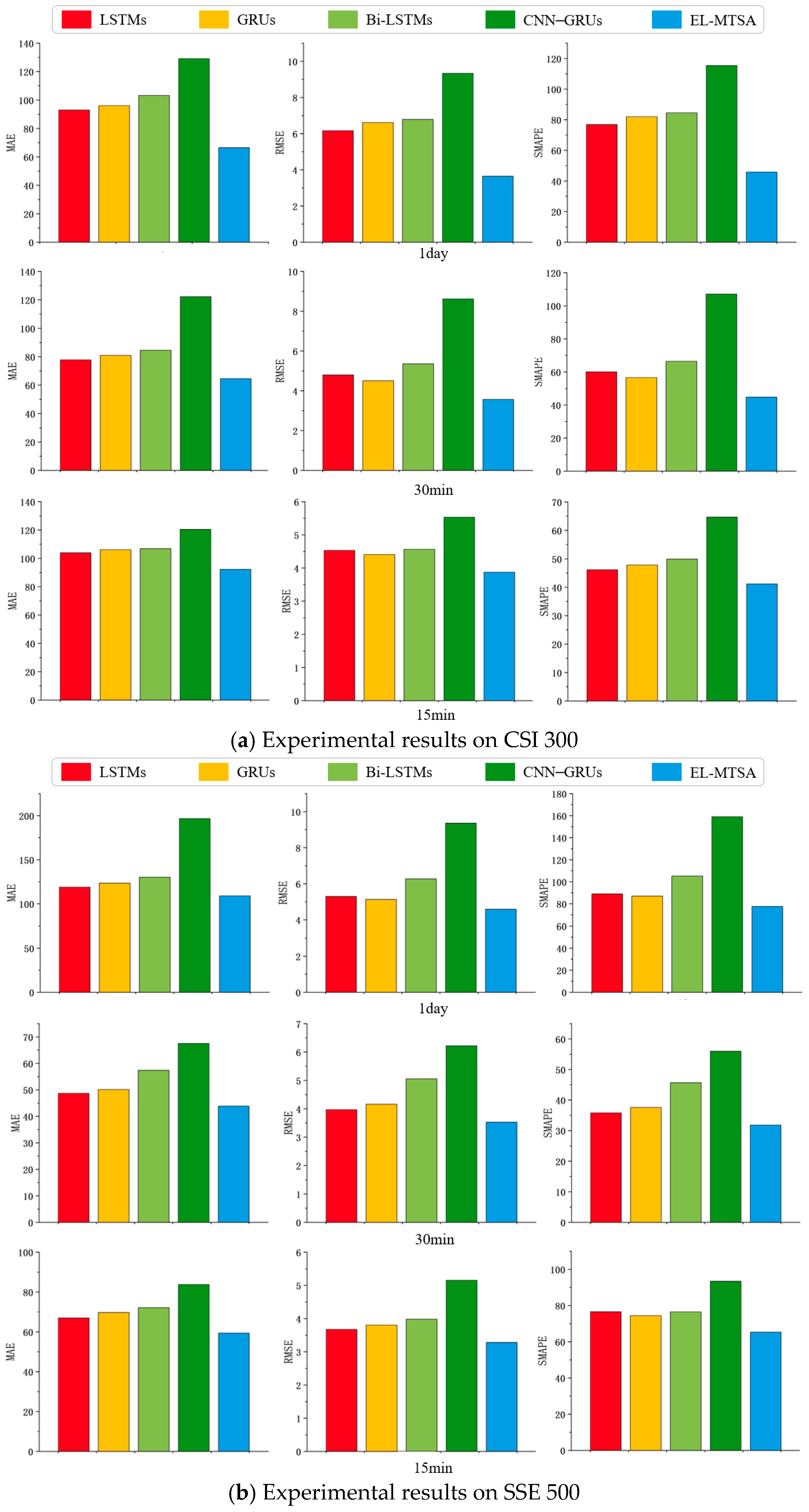
| Dataset | Model | MAE | SMAPE | RMSE |
|---|---|---|---|---|
| CSI 300 | LSTM | 103.2417 | 86.3657 | 6.9361 |
| LSTMs | 92.97682 | 76.8875 | 6.1656 | |
| GRU | 110.4894 | 94.0744 | 7.4454 | |
| GRUs | 96.11654 | 81.9423 | 6.6180 | |
| Bi-LSTM | 112.3565 | 98.4684 | 7.9174 | |
| Bi-LSTMs | 103.2319 | 84.5469 | 6.7844 | |
| CNN–GRU | 134.956 | 121.7692 | 9.8259 | |
| CNN–GRUs | 129.1301 | 115.4156 | 9.3368 | |
| SSE 500 | LSTM | 123.5744 | 87.2047 | 5.1516 |
| LSTMs | 118.9043 | 89.0538 | 5.2994 | |
| GRU | 131.2696 | 104.1869 | 6.1949 | |
| GRUs | 123.5361 | 87.0197 | 5.1353 | |
| Bi-LSTM | 133.6997 | 107.8816 | 6.4218 | |
| Bi-LSTMs | 130.2673 | 105.2568 | 6.2729 | |
| CNN–GRU | 220.4278 | 177.5467 | 10.3707 | |
| CNN–GRUs | 196.7126 | 159.0642 | 9.3620 | |
| CSI A50 | LSTM | 63.0576 | 51.7572 | 5.6813 |
| LSTMs | 56.9408 | 41.5815 | 4.6440 | |
| GRU | 63.4638 | 53.4567 | 5.9116 | |
| GRUs | 59.6080 | 41.0670 | 4.5420 | |
| Bi-LSTM | 76.4491 | 66.4530 | 7.2827 | |
| Bi-LSTMs | 69.2172 | 59.2439 | 6.5821 | |
| CNN–GRU | 82.5765 | 68.9709 | 7.5493 | |
| CNN–GRUs | 77.5468 | 65.1126 | 7.1062 |
| Dataset | Step | MAE | SMAPE | RMSE |
|---|---|---|---|---|
| CSI 300 | 1 | 80.33817 | 68.62665 | 4.066288 |
| 3 | 63.81433 | 45.47347 | 3.640053 | |
| 5 | 59.40408 | 41.17131 | 3.281625 | |
| 7 | 65.63917 | 47.11563 | 3.753997 | |
| 10 | 84.84073 | 68.62874 | 4.079142 | |
| 15 | 112.4575 | 77.06639 | 4.565558 | |
| SSE 500 | 1 | 112.3726 | 76.73992 | 4.537459 |
| 3 | 101.5696 | 71.50873 | 4.231308 | |
| 5 | 92.28185 | 65.31663 | 3.872534 | |
| 7 | 102.6991 | 74.36072 | 4.411835 | |
| 10 | 114.8737 | 85.40998 | 5.059516 | |
| 15 | 122.6164 | 84.45515 | 4.987733 | |
| CSI A50 | 1 | 45.54298 | 31.61423 | 3.498296 |
| 3 | 42.47965 | 29.35284 | 3.258542 | |
| 5 | 39.15164 | 27.08353 | 3.00892 | |
| 7 | 44.06771 | 31.8926 | 3.534709 | |
| 10 | 53.60153 | 41.20854 | 4.5633 | |
| 15 | 59.64439 | 49.61624 | 5.523892 |
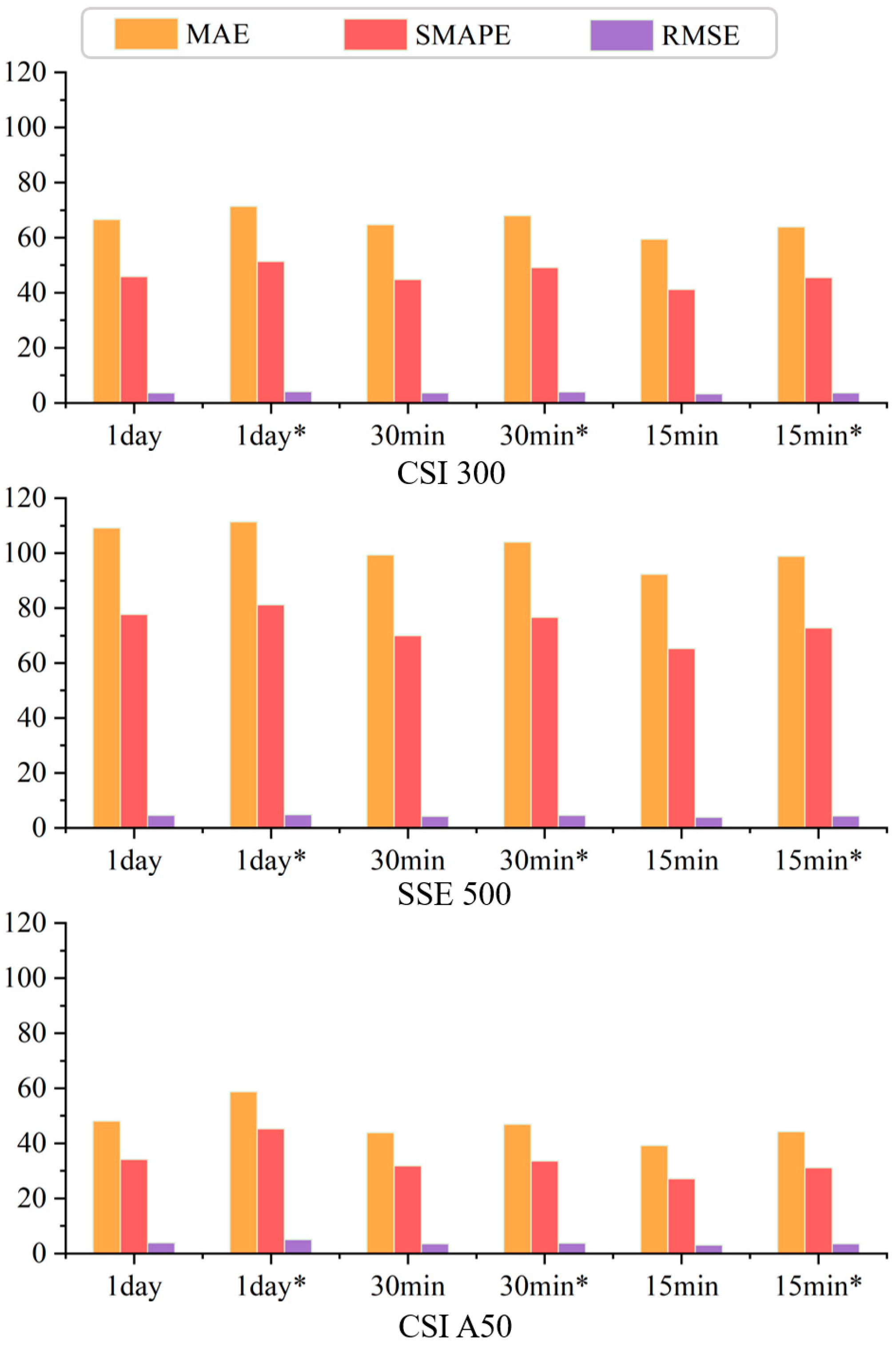
| Dataset | Model | Frequency | MAE | SMAPE | RMSE |
|---|---|---|---|---|---|
| CSI 300 | EL-MTSAs | 1 day | 66.53035 | 45.86216 | 3.645549 |
| EL-MTSAs | 30 min | 64.62842 | 44.8067 | 3.569873 | |
| EL-MTSAs | 15 min | 59.40408 | 41.17131 | 3.281625 | |
| EL-MTSAs * | 1 day | 71.38656 | 51.39556 | 4.099139 | |
| EL-MTSAs * | 30 min | 67.95656 | 49.08186 | 3.921806 | |
| EL-MTSAs * | 15 min | 63.81433 | 45.47347 | 3.640053 | |
| SSE 500 | EL-MTSAs | 1 day | 109.1481 | 77.69253 | 4.588616 |
| EL-MTSAs | 30 min | 99.29775 | 69.92445 | 4.142188 | |
| EL-MTSAs | 15 min | 92.28185 | 65.31663 | 3.872534 | |
| EL-MTSAs * | 1 day | 111.3266 | 81.13307 | 4.811939 | |
| EL-MTSAs * | 30 min | 103.9623 | 76.61262 | 4.531059 | |
| EL-MTSAs * | 15 min | 98.8652 | 72.78998 | 4.282745 | |
| CSI A50 | EL-MTSAs | 1 day | 48.05319 | 34.09183 | 3.78931 |
| EL-MTSAs | 30 min | 43.88325 | 31.81827 | 3.529929 | |
| EL-MTSAs | 15 min | 39.15164 | 27.08353 | 3.00892 | |
| EL-MTSAs * | 1 day | 58.76713 | 45.28799 | 5.016004 | |
| EL-MTSAs * | 30 min | 46.90205 | 33.49926 | 3.709601 | |
| EL-MTSAs * | 15 min | 44.21733 | 31.14188 | 3.452698 |
| Model | FPV | TP | SR | MDD |
|---|---|---|---|---|
| Buy-and-hold | 142,599.4903 | 42,599.4903 | 1.4195 | 0.15816 |
| Martingale model | 125,125.7755 | 25,125.7755 | 1.1583 | 0.10183 |
| EL-MTSA | 151,876.9812 | 51,876.9812 | 3.7597 | 0.03587 |
Disclaimer/Publisher’s Note: The statements, opinions and data contained in all publications are solely those of the individual author(s) and contributor(s) and not of MDPI and/or the editor(s). MDPI and/or the editor(s) disclaim responsibility for any injury to people or property resulting from any ideas, methods, instructions or products referred to in the content. |
© 2025 by the authors. Licensee MDPI, Basel, Switzerland. This article is an open access article distributed under the terms and conditions of the Creative Commons Attribution (CC BY) license (https://creativecommons.org/licenses/by/4.0/).
Share and Cite
Kong, J.; Zhao, X.; He, W.; Yang, X.; Jin, X. EL-MTSA: Stock Prediction Model Based on Ensemble Learning and Multimodal Time Series Analysis. Appl. Sci. 2025, 15, 4669. https://doi.org/10.3390/app15094669
Kong J, Zhao X, He W, Yang X, Jin X. EL-MTSA: Stock Prediction Model Based on Ensemble Learning and Multimodal Time Series Analysis. Applied Sciences. 2025; 15(9):4669. https://doi.org/10.3390/app15094669
Chicago/Turabian StyleKong, Jianlei, Xueqi Zhao, Wenjuan He, Xiaobo Yang, and Xuebo Jin. 2025. "EL-MTSA: Stock Prediction Model Based on Ensemble Learning and Multimodal Time Series Analysis" Applied Sciences 15, no. 9: 4669. https://doi.org/10.3390/app15094669
APA StyleKong, J., Zhao, X., He, W., Yang, X., & Jin, X. (2025). EL-MTSA: Stock Prediction Model Based on Ensemble Learning and Multimodal Time Series Analysis. Applied Sciences, 15(9), 4669. https://doi.org/10.3390/app15094669