Article

Patient-Tailored Dementia Diagnosis with CNN-Based Brain MRI Classification

The Institute of Computer Science, Faculty of Electronics and Information Technology, Warsaw University of Technology, Pl. Politechniki 1, 00-661 Warsaw, Poland
*
Author to whom correspondence should be addressed.
Appl. Sci. 2025, 15(9), 4652; https://doi.org/10.3390/app15094652
Submission received: 24 March 2025 / Revised: 17 April 2025 / Accepted: 21 April 2025 / Published: 23 April 2025
(This article belongs to the Section Applied Biosciences and Bioengineering)

Abstract

:

Featured Application

This study explores the potential application of CNN-based models for the automated diagnosis of dementia using MRI brain images. The developed models could be integrated into a CDSS that aids clinicians in the early detection of dementia, its subtype differentiation, and staging. Such a system could also guide personalized treatment strategies.

Abstract

This study explores the potential of using convolutional neural networks (CNNs) to diagnose dementia early and manage it in an individualized way. Segmented brain magnetic resonance imaging (MRI) images from the Alzheimer’s Disease Neuroimaging Initiative (ADNI) database represented Alzheimer’s disease (AD), mild cognitive impairment (MCI), and cognitively normal (CN) subjects. These classes served to train, validate, and test CNN-based models. The first four models were developed entirely from scratch, and the other four employed transfer learning (TL). While both approaches demonstrated high classification accuracy (93.69% on average), TL-based models outperformed independently developed ones, achieving 97.64% accuracy compared with 89.75%. The CNN-based models yielded information about detected dementia type, diagnosis confidence level, and gradient-weighted class activation mapping (Grad-CAM)-generated heatmaps highlighting pathologically affected brain regions. These results indicate the high potential of CNN-based models for enhancing early dementia detection and differentiation and offer a promising basis for developing deep learning (DL)-based clinical decision support systems (CDSSs). Such systems could assist healthcare professionals in reducing dementia diagnosis time, optimizing patient-tailored management and treatment strategies, and improving the quality of life for individuals with dementia.

1. Introduction

1.1. Initial Considerations

Dementia is a neurocognitive disorder with multiple forms with varying degrees of severity. It encompasses a spectrum of symptoms resulting from different diseases or traumas. It leads to progressive neurodegeneration and significant cognitive decline, interfering with an individual’s daily life. Dementia typically involves memory impairment, disruption in thought patterns, behavioral problems, and diminishing motor control. Other common symptoms include emotional volatility, linguistic difficulties, social withdrawal, and decreased motivation [1].
Currently, over 55 million people worldwide are living with dementia, and nearly 10 million new cases are diagnosed annually. It is the seventh leading cause of death and a major contributor to disability among the elderly globally [2].
There is currently no known cure for dementia, and the available treatment options are most effective if administered early, before the onset of symptoms [1,3]. Unfortunately, most patients begin therapy when their daily functioning is already significantly impaired, at which point, treatment often does not yield optimal outcomes [4].
Alzheimer’s disease (AD) accounts for 60% to 70% of all dementia cases worldwide, affecting roughly one in ten individuals over 65 and nearly a third of those over 85 [2]. Research suggests that AD progresses silently for decades before noticeable clinical symptoms emerge, with typical brain atrophy patterns appearing first in the medial temporal lobes [1,5,6].
Some individuals with these early signs develop mild cognitive impairment (MCI), an intermediate stage between normal aging-related cognitive decline and AD dementia, where memory deficits exceed those present in cognitively normal (CN) individuals but still remain insufficiently severe to disrupt daily functioning [7].
AD poses a significant diagnostic challenge due to its diverse clinical presentation across patients [8]. Early and accurate detection, particularly at the MCI stage, is essential for timely intervention, effective symptom management, and improved treatment outcomes [7,9].
Standard diagnostic methods for dementia typically include clinical evaluations, neuropsychological assessments, cognitive testing, cerebrospinal fluid (CSF) and blood biomarker analysis, and neuroimaging [10]. While these approaches provide valuable insights, they are often expensive, invasive, time-consuming, and dependent on highly skilled specialists [11].
Magnetic resonance imaging (MRI), particularly T1-weighted structural scans, plays a pivotal role in diagnosing and monitoring AD, MCI, and other dementias. Its high spatial resolution makes it the preferred method for detecting early neurodegenerative changes such as hippocampal atrophy and cortical thinning, two of the better-established structural biomarkers of dementia progression [12].
Hippocampal atrophy is widely recognized as a hallmark of early AD pathology, often preceding the onset of cognitive symptoms [13]. Cortical thinning, especially in the temporoparietal and medial temporal regions, correlates with both disease severity and the risk of conversion from MCI to AD [14]. These changes offer objective, quantitative metrics that help differentiate between CN individuals, MCI patients, and those with AD.
Recent advances in artificial intelligence (AI) have further enhanced the diagnostic value of neuroimaging and the utility of its associated biomarkers, leading to the development of robust predictive frameworks for dementia [15]. AI-based tools can detect subtle, spatially distributed atrophy patterns, such as microstructural changes in the hippocampal region and focal cortical thinning, often before cognitive decline becomes evident [16]. These biomarkers constitute precise and quantifiable measures of neurodegeneration, making them accurate key early indicators [17]. They not only support individualized disease monitoring and prognosis but also directly contribute to improved patient outcomes [18].
Recently, deep learning (DL) techniques, particularly convolutional neural networks (CNNs), have emerged as powerful tools for detecting and analyzing dementia-specific biomarkers [19]. By processing extensive radiological datasets, CNN-based models capture intricate neurodegeneration patterns, enabling accurate disease progression predictions [20,21]. Their application extends beyond diagnosis, facilitating the development of personalized treatment strategies [22,23].
Traditional machine learning (ML) algorithms such as support vector machines (SVMs), random forests, and boosting methods have long been used for dementia classification tasks. Variants of SVMs have previously been proposed to improve performance [24]. However, all these approaches generally rely on manually extracting regions of interest (ROIs) based on known MRI brain biomarkers, which is time-consuming and subjective given the absence of universally agreed-upon dementia biomarkers. As a result, conventional models may fail to capture the full complexity of AD presentation and are often limited by labor-intensive feature engineering and risk of overfitting [25].
DL offers a more scalable and data-driven alternative. Architectures such as CNNs, recurrent neural networks (RNNs), and autoencoders can learn discriminative features without manual input [24,26]. Among these, CNNs have become the most widely adopted for AI-driven neuroimaging analysis due to their ability to exploit spatial hierarchies in image data, reduce complexity via weight sharing, and operate directly on image slices [27]. Notably, CNNs trained on 2D axial MRI slices have demonstrated strong generalization across scanners and protocols. Models such as pre-trained AlexNet and VGG-16 have achieved classification accuracies as high as 99.21% and 95.73%, respectively [24,25].
Beyond standard CNNs, recent studies have incorporated mechanisms to improve the localization of informative brain regions. Adaptive hybrid networks such as those proposed by Illakiya et al. [28], which integrate non-local and coordinate attention modules, have achieved classification accuracies of up to 98.53%. Similarly, Zhang et al. [29] developed a multimodal framework combining 3D attention with ResNet to improve diagnostic accuracy for both AD and MCI. Other works have integrated CNNs with transformer architectures and novel attention-based fusion strategies to model local and global contextual features better [25,30].
To overcome the limitations of 2D models, such as the loss of inter-slice spatial continuity, researchers have begun to explore volumetric modeling using 3D CNNs. For example, Kang et al. [31] introduced a 3D generative adversarial network with a three-round learning strategy, achieving 92.8% accuracy in binary classification tasks. Zhang et al. [29] extended this by integrating multimodal data into a 3D ResNet framework, outperforming single-modality models by 3–6%. Liu et al. [32] explored multiscale image patching centered on anatomical landmarks to improve training efficiency, while Lian et al. [33] proposed a hybrid network that extracts multi-level discriminative features from entire MRI volumes, balancing global and local structural information.
Some approaches have focused on isolating specific brain structures prior to classification. Poloni and Ferrari [34], as well as Cui and Liu [35], investigated targeted regions, such as the hippocampus, to enhance AD and MCI differentiation. Chen and Xia [36] introduced a sparse regression module to identify critical cortical areas, such as the posterior temporal lobe, prior to DL-based classification, improving accuracy through spatially constrained feature extraction. Although effective, these targeted methods often involve complex segmentation steps that may limit scalability.
Despite these advances, significant challenges persist in deploying 3D DL models in clinical contexts. These include high computational costs, memory demand, and the need for large labeled datasets. Many current models also underutilize complementary features across views, extracting data from isolated patches, which may result in loss of global context. To address these trade-offs, our study focuses on optimizing 2D CNN architectures for efficiency and generalizability while laying the foundation for future integration of volumetric and attention-based techniques.
Although 2D CNNs offer a practical and high-performing baseline for dementia classification using MRI, the field is rapidly evolving toward more sophisticated architectures that integrate spatial, temporal, and multimodal information. As research progresses, future models are likely to incorporate attention mechanisms, region-specific modeling, feature fusion strategies, and 3D analysis to further enhance diagnostic accuracy and clinical applicability.

1.2. Research Aims

  • The primary objectives of this study were as follows:
  • To demonstrate how CNN-based models can aid clinical decision-making for dementia patients;
  • To utilize dementia-specific neuroimaging biomarkers to detect brain atrophy at the earliest possible stage and monitor disease progression from MCI to AD;
  • To support the use of the DL tools for the development of personalized dementia care plans.
  • The innovations of the proposed approach include the following:
  • A lightweight 2D-CNN architecture That employs an optimized, low-complexity 2D-CNN model to balance diagnostic accuracy with reduced computational cost and memory usage;
  • A single-slice classification strategy that implements a slice-wise classification approach using a single representative MRI slice per subject, minimizing data redundancy and model overfitting;
  • An efficient training process that reduces training time significantly compared with volumetric 3D models, facilitating rapid experimentation and model adjustment;
  • Robust performance on limited data, achieving high diagnostic accuracy despite limited labeled data, demonstrating strong generalization capabilities;
  • Potential for real-time use, whereby the low computational burden and fast inference time make the model suitable for integration into real-time clinical research frameworks.

2. Materials and Methods

2.1. Data Collection and Preliminary Analysis

2.1.1. Data Sources

The data used in this study were obtained from the Alzheimer’s Disease Neuroimaging Initiative (ADNI) database (https://adni.loni.usc.edu/, accessed on 15 May 2024) after completing the standard application and approval process [37], including the ADNI Data Use Agreement. All data were provided in de-identified form, per ADNI’s ethical and data-sharing policies. Informed consent was obtained from all participants, and ethical approval was granted by the relevant institutional review boards at participating sites.
While the processed dataset generated for this study cannot be made publicly available due to data use restrictions, researchers interested in accessing the original ADNI data can do so by registering through the official portal and following the established procedures.
As detailed in Table 1, the data were collected from participants of different ages and genders in the form of anonymized, high-resolution T1-weighted 3D magnetization-prepared rapid gradient-echo (MPRAGE) brain scans obtained from 1.5T MRI units. The participants were assigned into three main research groups as follows, depending on their diagnosis:
  • AD—individuals diagnosed with AD and exhibiting typical signs and symptoms;
  • CN—control group of CN subjects exhibiting no signs of dementia;
  • MCI—individuals with subjective cognitive impairment of varying severity but without any other typical signs of dementia, whose daily activities remained mostly unaffected.

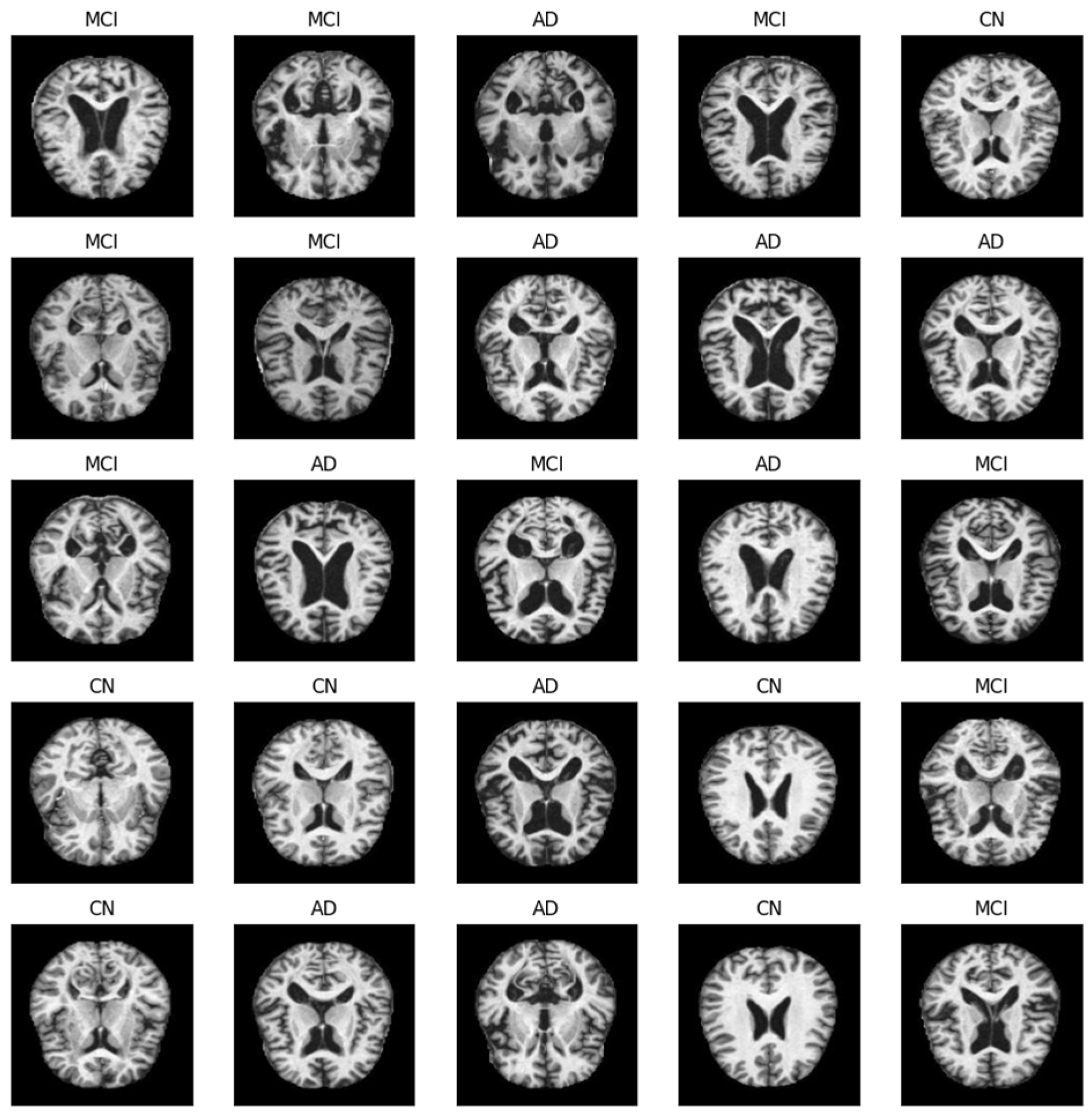
2.1.2. Data Preprocessing and Selection

FreeSurfer (Version 7.4.1), a specialized neuroimaging software, was used for skull-stripping and segmentation of the MRI brain scans into volumes of interest (VOIs) [38].
The data were labeled and categorized into three distinct classes: CN, MCI, and AD, corresponding to the type of dementia as well as characteristic brain atrophy patterns. The labels were then used to sort the files into three directories, ensuring an organized structure for subsequent analysis.
The segmented and labeled brain VOIs were initially stored as Neuroimaging Informatics Technology Initiative (NIfTI) files. They were all then converted into two-dimensional JPEG representations, as shown in Figure 1, using NiBabel and Nilearn libraries. From each 3D brain volume, exactly 50 contiguous middle slices in the axial orientation were extracted. This specific range was selected because central axial slices are more likely to capture brain regions where typical neurodegeneration indicative of early dementia occurs, such as ventricular enlargement, cortical thinning, and atrophy of the medial temporal lobe. This particular number of slices was chosen to balance anatomical coverage with computational feasibility and operational resources.
The processing resulted in 4060 JPEG files per class (AD, MCI, and CN), totaling 12,180 two-dimensional brain-representative ROIs used as normalized inputs. The ROIs were then randomly assigned into training, validation, and testing sets—3200 images per class for training, 800 for validation, and 60 for testing.
The brain ROIs were randomly distributed into training, validation, and testing sets. 3200 JPEG images per class (AD, MCI, CN) were allocated for training, 800 for validation, and 60 for testing.

2.2. CNN-Based Models for Diagnostic Support of Dementia

2.2.1. Used Tools and Software

The CNN models used for the classification task were developed using the Python (Version 3.12.3) programming language in the Google Colab and Spyder integrated development environments.
Key libraries utilized included TensorFlow (Keras) (Version v2.16.1), Matplotlib (Version 3.9.0), NumPy (Version 1.26.0), SciPy (Version 1.13.1), Scikit-learn (Version 1.5.0), OpenCV (Version 4.9.0), Pandas (Version 2.2.2), and Pillow (10.3.0).

2.2.2. Independently Developed CNN-Based Models

The independently developed models tackling the medical image classification task were constructed from scratch based on conventional CNN architecture, which included convolutional, pooling, normalizing, dropout, flattening, and dense layers.
The input layer accepted the RGB 192 × 192 pixel brain-representative ROIs.
Convolutional (Conv2D) layers were the most essential components of the independently developed CNN-based models. They employed the rectified linear unit activation function, which enabled the models to learn more complicated patterns. The models varied in terms of the numbers of Conv2D layers and filters used within them, as detailed in Table 2. It was hypothesized that increasing the number of consecutive Conv2D layers and hence, the number of filters would allow the model to extract and refine more detailed features from the inputs, thus resulting in improved classification performance.
The output layer employed the softmax activation function to generate a three-element vector, with each element reflecting the predicted probability of the output belonging to one of the three classes (AD, CN, and MCI).

2.2.3. CNN-Based Models TL

This study also aimed to compare the performance of the previously described group of models with those constructed using transfer learning (TL) based on pre-trained CNN architectures, such as ResNet50 [39], Xception [40], MobileNet [41], and VGG16 [42], as shown in Table 3.
The lower half of each pre-trained model was frozen, leaving only the top layers available for fine-tuning. This approach allowed the TL-based models to retain the lower-level features learned from the ImageNet dataset while adapting the higher-level features to the specifics of the brain-representative ROIs explored in this study.
New layers were added on top of each TL-based model (identical across all models) to ensure consistency and reproducibility of the outputs.
A GitHub “https://github.com/ZKnapinskaWUT/Patient-Tailored-Dementia-Diagnosis-with-CNN-Based-Brain-MRI-Classification/tree/main (created and accessed on 17 April 2025)” repository was created to share code related to all the CNN architectures explored in the study, including their structure and key functionalities.

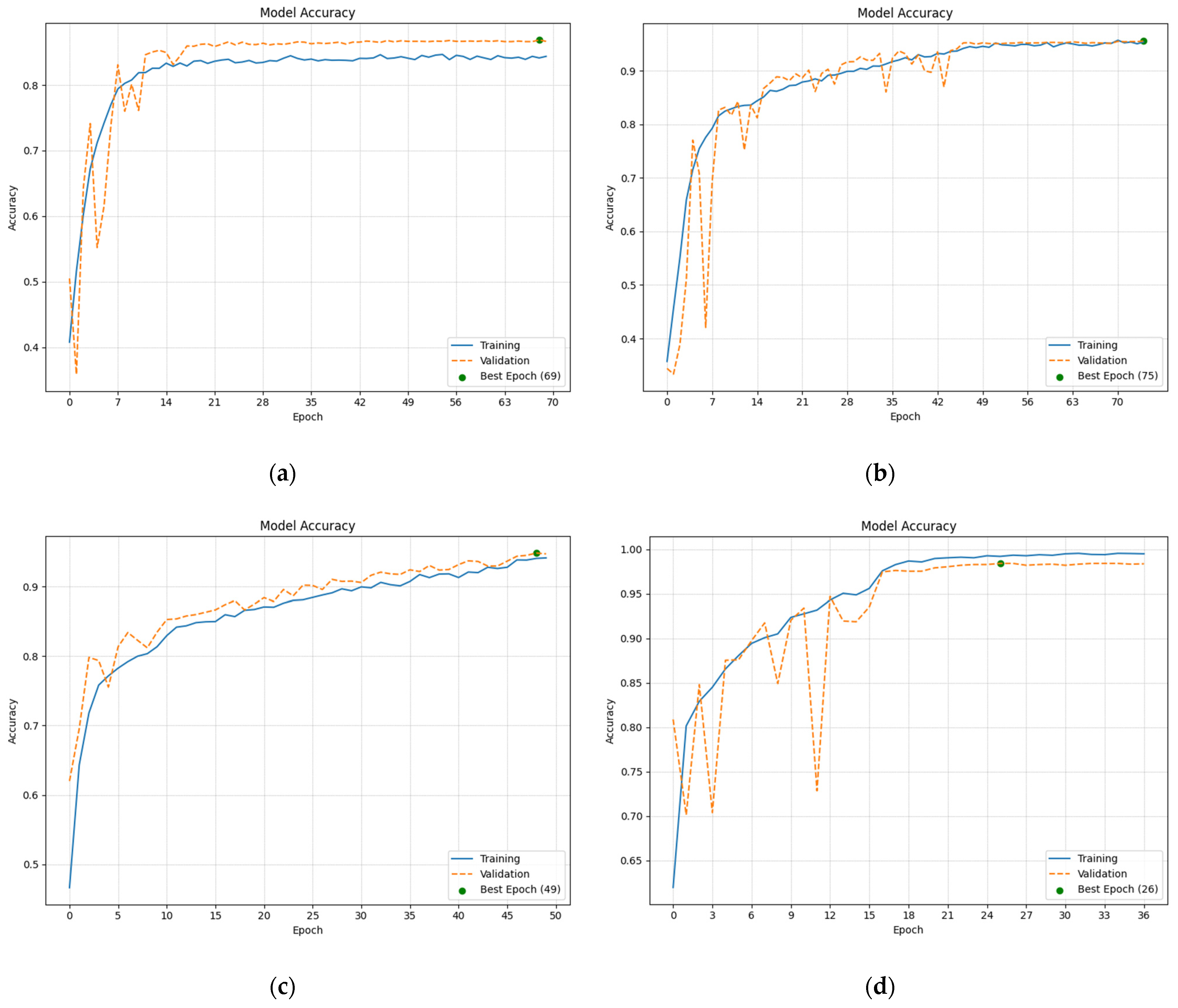
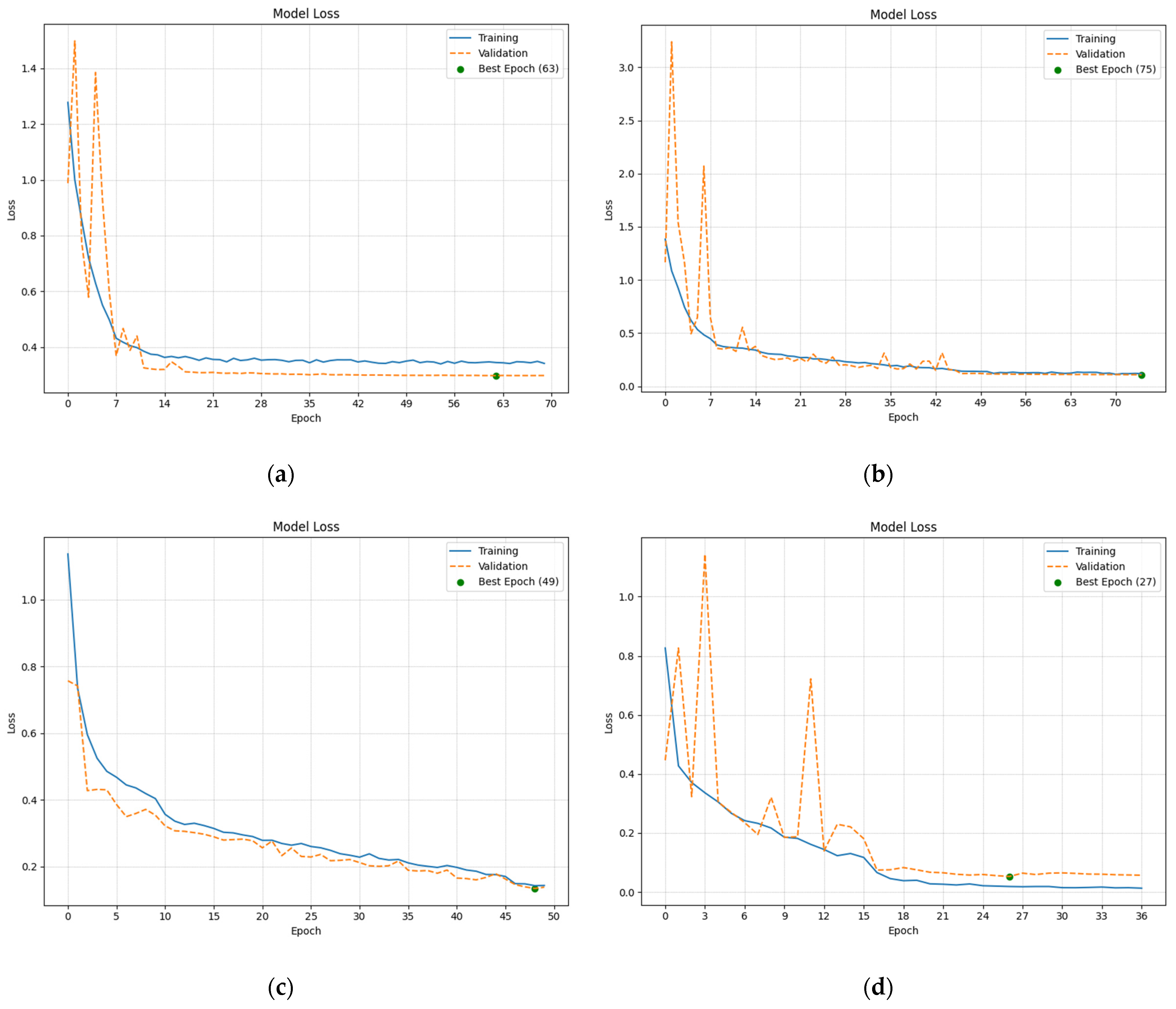
2.2.4. Analysis of the Training and Validation

The metrics chosen to evaluate the models’ performance during training and validation included accuracy and loss. These values were calculated for each epoch.
All CNN-based models demonstrated high accuracy, with the independently developed ones achieving values of over 90% and the TL-based models exceeding 95%, as depicted in Figure 2. These high rates indicate that all the models were well suited for the classification task and input data, yielding generally correct predictions, both during training and validation.
The accuracy curves exhibited an exponential-like growth. In some cases, the value of validation accuracy exceeded training accuracy. This was due to the data preparation process, as the training batch underwent augmentation while the validation batch remained as it was originally. The epochs at which the highest accuracy values were achieved are marked with a green dot.
A clear difference was observed between the independently developed and TL-based models. The first group reached peak accuracy much later than the second. Furthermore, models with more layers and deeper structures exhibited smoother and less erratic accuracy curves.
The loss curves plotted using loss function values over subsequent epochs during training and validation showed a logarithmic-like decrease, as shown in Figure 3. Independently developed models achieved loss values of around 0.3, and TL-based models reached values below 0.2. Such low values suggest that all models made more correct predictions than incorrect ones and did not overfit the data.
Notably, the curves did not increase again after stabilizing, indicating that the models retained their generalization ability. Models with more layers and complex, deeper structures exhibited smoother and less erratic loss curves.
The epochs at which the lowest loss values were achieved are marked with a green dot. A notable difference was observed between the independently developed models and Tl-based ones; the former reached their lowest loss values much later than the latter.

3. Results

3.1. Evaluation of the Diagnostic Ability of the CNN-Based Models

The general performance of all models was evaluated using several classification quality metrics, such as accuracy (ACC), precision, recall, F1 score, confusion matrix, Matthews correlation coefficient (MCC), receiver operating characteristic (ROC) curve, and area under the ROC curve (AUC) score.
Evaluating the classification quality metrics across all developed CNN-based models, as shown in Table 4, it is evident that they all significantly exceeded the 50% threshold, thereby demonstrating robust predictive capability across AD, CN, and MCI classes.
Precision, quantifying the proportion of correctly predicted positive observations among all predicted positives, ranged from 83% to 100% on average. This indicates that the models consistently returned high proportions of true positives relative to false positives, with the strongest results observed in the VGG16-based and MobileNet-based models (100% and 98%, respectively).
Regarding recall (sensitivity), most models demonstrated satisfactory performance, with average values ranging from 82% to 100%. Again, this indicates that the models were generally reliable in detecting the true cases in each class, including unseen testing inputs.
The F1 score, which correlates precision and recall into a single metric, followed the same trend, ranging from 81% to 100% on average across the models. The consistency among these three metrics supports the stability and general reliability of the classifiers explored in this study.
ACC and MCC were computed to further account for class imbalance and provide a more objective, reproducible measure of predictive performance.
Average ACC values ranged from 81.67% (Custom CNN 128) to a perfect 100% (VGG16-based), reflecting strong overall performance. Notably, all CNN-based models exceeded the 80% threshold, with several, such as the Custom CNN 1024, Xception-based, and MobileNet-based models surpassing 95%.
The MCC, which incorporates true and false positives and negatives into a single correlation metric and is particularly useful in multiclass contexts, showed a similarly strong performance, ranging from 73.27% to 100% across all the tested models. The VGG16-based model again achieved the maximum value here, indicating an ideal correlation between predicted and actual labels.
AUC was calculated to assess the discriminative power of the models comprehensively. This metric provides insight into a model’s ability to distinguish between classes across varying thresholds. Average AUC values ranged from 0.86 to 1.00, with five models (Custom CNN 1024, ResNet50-based, Xception-based, MobileNet-based, and VGG16-based) exceeding 0.95. The VGG16-based model achieved perfect AUC scores (1.00) for all classes.
The values of the classification quality metrics revealed variability not only across different models but also among the image classes. The values of the metrics for the AD class were consistently perfect, with each model achieving 100% across all assessment categories (precision, recall, F1 score, accuracy, and AUC). Such flawless performance is rare in real-world scenarios, and the reasons for this outcome are unclear. One hypothesis is that the data for the AD class may have had lower variability, leading the models to overfit it. Alternatively, it is possible that the images belonging to the AD class possessed distinct and unique characteristics that were easily recognized and learned by the models, resulting in consistently accurate classification.
All models performed well in the CN and MCI classes. However, the latter posed the greatest classification challenge, which is likely to have been due to the inherent heterogeneity and overlapping imaging features of MCI subtypes. This complexity makes it difficult for the models to establish a consistent visual representation, affecting their ability to categorize MCI inputs accurately. Still, performance in relation to this class remained high, particularly for the Custom CNN 1024, Xception-based, MobileNet-based, and VGG16-based models, which achieved accuracy values of 86.7%, 93.3%, 95%, and 100%, respectively.
The VGG16-based model achieved perfect performance, with classification quality scores reaching 100% across all evaluation metrics. Such results are uncommon in real-world scenarios and suggest that the model may have overfitted the data, potentially due to its shallow architecture with just 16 base layers. It could also imply that the model reached its maximum processing capacity and could not appropriately handle the higher dimensionality and complexity of the image features.
The confusion matrices for all the CNN-based models exhibited a high frequency of true positive classifications in all three classes, as depicted in Figure 4. All ROC curves across different thresholds lean strongly toward the upper-left corner of the plot. Both of these observations indicate that the predictions the models yielded during testing were accurate and not random.
Notably, the ROC curve for the AD class is ideal, positioned precisely in the upper-left corner of the plot. The models’ performance regarding two other classes, CN and MCI, was still objectively satisfactory. Both corresponding ROC curves were similar and spatially close to each other across all plots.
Among the custom-developed models, the Custom CNN 1024 performed best, reaching 100% ACC for AD and CN classes and achieving a micro- and macro-average AUC of 0.97, making it the top performer in this group. Within the group of the TL-based models, the VGG16-based model showed flawless performance across all classification quality metrics (precision, recall, F1 score, ACC, and AUC), without any misclassification. The Xception-based and MobileNet-based models also demonstrated outstanding results, achieving near-perfect ROC curves and micro-/macro-average AUC values of 0.98 and 0.99, respectively.
Comparing the confusion matrices and ROC curves of independently developed models with those of TL-based models, it was evident that the latter group performed slightly better. The average classification ACC of the TL-based models was very high. The AUC values were also consistently greater in the case of TL-based models.
Overall, the inclusion of multiple varied evaluation metrics provides a comprehensive view of model performance. These results affirm that the CNN-based architectures, especially the TL-based ones, exhibit excellent potential in the automated classification of dementia-related neuroimaging data.

3.2. Proposed CDSS for Dementia Grad-CAM

Grad-CAM, a class-discriminative localization technique designed to enhance the interpretability of CNN-based models’ outputs, was employed in this investigation. The method produced class-specific feature maps, visualized as heatmaps overlaying the output images, highlighting the regions relevant to the prediction [43].
The objective was to determine whether the highlighted areas aligned with the neurodegenerative patterns of brain atrophy associated with either MCI or AD as documented in the medical literature.
It was observed that models with a deeper structure and, hence, more convolutional layers (with more filters within them) generally output more accurate predictions and better localized the brain atrophy patterns with the heatmaps, as shown in Figure 5.
The highlighted areas often corresponded with key structural biomarkers of dementia. Specifically, Grad-CAM frequently emphasized the periventricular regions, suggestive of ventricular enlargement, and the medial temporal lobes, where hippocampal volume loss and cortical thinning are typically most pronounced in MCI and early AD. The heatmap visualizations closely reflected the known patterns of structural neurodegeneration, particularly in temporoparietal regions.
Cortical thickness measures, particularly when computed using tools such as FreeSurfer or ANTs, offer sub-millimeter precision in detecting focal cortical atrophy [13]. In parallel, a change in the hippocampal volume remains one of AD’s most well-established imaging biomarkers, though its interpretation typically requires readjustment for head size. While Grad-CAM was not explicitly integrated with the mentioned quantitative measures in this particular experimental approach, its potential to complement structural biomarkers is promising. Future research could explore how co-analyzing Grad-CAM visualizations with cortical thickness and volumetric hippocampal data may enhance interpretability and provide more nuanced insights into a CNN-based dementia diagnosis.
As shown in Figure 6, the model output included the predicted dementia classification (type) paired with the confidence score and suggested optimal clinical management, further supporting clinical decision-making.

4. Discussion

This investigation aimed to assess the potential of CNN-based models in developing an optimal CDSS, specifically facilitating the early detection of dementia-related brain atrophy patterns in structural MRI scans.
Overall, the TL-based models outperformed the independently developed ones, although the difference was not major. This superior performance may be attributed to the TL-based models’ more complex and deeper structures, except the VGG16-based one, which was relatively shallow. Using TL for model construction generally ensures that the weights are already optimized for multidimensional image classification, which makes the training easier and more efficient.
These models achieved near-perfect results, with AUC scores of 0.96–1 and average ACC values exceeding 94%, underscoring their high discriminative power, generalizability, and the ability to extract subtle patterns in neuroimaging data relevant to dementia diagnosis.
The independently developed models also delivered satisfactory performance, particularly those with more convolutional layers and filters, confirming that deeper architectures are more effective at learning from high-dimensional MRI imaging data.
The best-performing custom CNN-based model (Custom CNN 1024) reached an average ACC of 95.56% and an AUC of 0.97 and maintained a strong precision–recall balance across all classes, suggesting that well-designed, task-specific CNNs can rival more complex TL-based architectures when trained appropriately.
The Grad-CAM analysis of the predictions generated by the CNN-based models revealed that the highlighted brain regions were predominantly located around the ventricles and in the medial parts of the temporal and parietal lobes.
The more complex the model’s structure was, the more focused and accurate these heatmaps became. The highlighted regions corresponded to characteristic atrophy patterns observed in dementia, particularly AD, including ventricular enlargement, cortical thinning, and medial temporal lobe (hippocampal) atrophy. These findings align closely with well-established neuroimaging biomarkers described in the medical literature. While the highlighted areas were not always perfectly localized, the overall pattern was consistent with known pathological changes, reinforcing the model’s potential for aiding in dementia diagnosis.
The Grad-CAM findings could provide valuable guidance for further examination and clinical management, suggesting specific brain regions that clinicians should investigate in greater detail. Since different stages of dementia exhibit distinct patterns of neurodegeneration with varying severity, the localization of the Grad-CAM-highlighted regions and the intensity of pathological changes could provide crucial insights for diagnosis, disease management, and treatment planning. This approach supports patient-tailored dementia care by refining the assessment of dementia progression.
To situate Grad-CAM within the broader context of interpretability techniques for CNN-based models, it is helpful to consider complementary methods such as LIME (local interpretable model-agnostic explanations) [44], SHAP (Shapley additive explanations) [45], and its extension, Shap-CAM [46]. These methods offer alternative perspectives on model decision-making by providing spatially resolved visual explanations, which are especially valuable for a more in-depth understanding of how the predictions are made.
LIME explains individual predictions by constructing local surrogate models based on input perturbations. For image data, it segments an image into interpretable regions (“superpixels”) and systematically masks them to assess their influence on the model’s output. This makes LIME applicable to CNNs without requiring access to the internal layers. However, LIME tends to struggle with stability and consistency when analyzing high-dimensional inputs such as medical imaging data, where subtle variations can lead to entirely different diagnoses [44,47].
SHAP takes a game-theoretic approach, assigning contribution scores to input features based on Shapley values. It offers consistency and theoretical robustness. However, its application to image data is hindered by high computational cost and the assumption of feature independence, which is not true in pixel-wise correlated MRI scans [45,48].
Shap-CAM, developed as a SHAP-based application for CNNs, attempts to account for spatial dependencies and produces saliency maps through marginal contribution analysis. While promising, it remains computationally intensive and conceptually complex [46].
In contrast, Grad-CAM is designed explicitly for convolutional architectures, making it particularly well-suited for medical imaging applications. By using the gradients flowing into the final convolutional layers, Grad-CAM highlights class-discriminative regions in a visually intuitive manner [43]. It preserves the spatial hierarchy of CNNs and provides clinically meaningful heatmaps that localize the brain regions that contribute most to the model’s decision. In dementia diagnosis, where identifying subtle structural abnormalities is crucial, Grad-CAM offers practical and focused interpretability balancing clarity, computational efficiency, and diagnostic relevance more effectively than other attribution methods.
Nevertheless, combining Grad-CAM with techniques such as LIME or SHAP could further enrich model transparency by revealing different aspects of model behavior. Integrating multiple interpretability tools in future studies may enhance clinicians’ trust in the model and guide its development by combining insights across spatial, feature-level, and local decision boundaries.

4.1. Study Limitations

The models developed in this study were limited to analyzing 2D representations of structural MRI brain scans, using normalized axial slices to simplify processing and reduce computational demands. This approach ensured consistency and reproducibility across the dataset, making it suitable for a proof-of-concept classification framework designed primarily for research purposes.
However, converting 3D (volumetric) MRI data into 2D slices inevitably results in losing some part of the spatial information.
Dementia-related neurodegeneration affects multiple brain regions, such as the hippocampus, medial temporal lobes, and parietal cortex, in a spatially complex and heterogeneous manner. The atrophy patterns can either be dispersed throughout the entire brain volume or localized in several specific anatomically distinct regions, making the 2D approach insufficient for capturing the full extent and distribution of these changes.
While suitable for preliminary experimentation, the models developed may not satisfy the requirements of real-life clinical applications, where a comprehensive spatial context is necessary for accurate diagnosis.
In this regard, 3D CNNs offer a promising alternative, as they can directly analyze volumetric brain data and capture the intricate spatial patterns of atrophy and pathological changes across the whole brain. Furthermore, techniques like voxel-based morphometry (VBM) have also been explored for dementia research to identify statistically significant regional differences in gray and white matter volume between symptomatic patients and CN individuals [49,50]. Incorporating VBM into the classification framework could enable a voxel-wise, whole-brain assessment of structural changes, which is particularly valuable in cases where the atrophy is subtle, diffuse, and not confined to predefined ROIs [51,52].
Future work will explore the application of 3D CNN-based models and assess the diagnostic utility of incorporating additional anatomical planes, such as sagittal and coronal, to understand better the contribution of different spatial orientations to the models’ classification performance and diagnostic accuracy. Integrating DL-based models with insights from established neuroimaging techniques such as VBM may enhance both performance and interpretability, contributing to more robust and clinically meaningful applications.
Additionally, in the context of dementia diagnosis, relying solely on imaging findings to construct a robust CDSS is not feasible. Although complex volumetric analyses, which involve extracting and processing radiomic features, can play a significant role in such a system, it is essential to recognize that the diagnostic process for dementia is multifaceted. It requires not only neuroimaging but also various cognitive assessments, laboratory testing results, and the detection of specific biomarkers (in blood, CSF, and even genes). These factors represent a fraction of the broader patient profile that must be considered for a comprehensive evaluation.
Although the findings of this exploration may not yet be directly applicable in real-life clinical settings, they provide a strong foundation for further research and development in the area of a potential AI-based dementia-related CDSS. Despite their limitations, they can still deliver essential insights and help guide clinicians in selecting more specialized diagnostic tests, potentially improving the accuracy of dementia diagnosis, speeding it up, and optimizing the quality of disease management.

4.2. Added Value

Early detection of neurodegenerative patterns within the brain is critical for the management of all dementia types, as the available pharmacological and non-pharmacological interventions are typically most effective precisely during either the preclinical or prodromal stage of the disease. If a model can accurately identify and highlight the early pathological changes, it could speed up or refine the diagnostic process, enabling patients to receive the most appropriate treatment much sooner.
In this investigation, a strong focus was placed on how the models approached the inputs representative of the MCI class. While this class posed a challenge for image classification due to its internal diversity, the models still demonstrated objectively strong performance, which can be deemed promising for future research.
For MCI, the accuracy, F1 scores, and AUC values are consistently above 60%, 69%, and 0.76, respectively, indicating a valuable potential for refining MCI detection.
When medical data are carefully curated and the study objectives are clearly defined, DL methods, specifically CNNs, can be effectively integrated into dementia management workflows. CNN-based models can speed up medical procedures, enhance patient comfort, and assist clinical personnel by reducing subjectivity and the risk of diagnostic errors. They provide physicians with filtered-out, clinically meaningful insights, thus flagging early pathological signs and supporting more accurate and timely decision-making.

4.3. Future Development Potential

An enhanced model design could significantly benefit from integration with scalable brain atlas frameworks and diagnostic scales based on imaging biomarkers for dementia. Incorporating this additional information could improve the model’s ability to accurately localize regions of neurodegeneration and atrophy across the entire cerebral volume. Furthermore, if such a hypothetical model were to incorporate knowledge from diagnostic scales effectively, it could relate detected image features to specific types and stages of dementia with high accuracy. This would provide a more detailed and clinically relevant perspective, offering valuable diagnosis and disease management insights.

5. Conclusions

The findings of this investigation demonstrate the feasibility and potential of CNN-based models for supporting early dementia diagnosis. Specifically, our approach shows promising accuracy in classifying MRI brain scans and localizing disease-relevant regions, laying the groundwork for a clinically applicable CDSS. In clinical practice, such a system could assist radiologists and neurologists by enhancing diagnostic precision, facilitating earlier intervention, and supporting individualized treatment strategies. These results provide a strong foundation for future research focused on refining model interpretability, integrating clinical scales, and ensuring scalability for real-world deployment.

Author Contributions

Conceptualization, Z.K. and J.M.; methodology, Z.K.; software, Z.K.; validation, J.M.; formal analysis, Z.K.; investigation, Z.K. and J.M.; resources, Z.K.; data curation, Z.K. and J.M.; writing—original draft preparation, Z.K.; writing—review and editing, J.M.; supervision, J.M.; project administration, J.M. All authors have read and agreed to the published version of the manuscript.

Funding

This research received no external funding.

Institutional Review Board Statement

Not applicable.

Informed Consent Statement

Not applicable.

Data Availability Statement

Data used in the preparation of this article were obtained from the Alzheimer’s Disease Neuroimaging Initiative (ADNI) database “https://adni.loni.usc.edu/ (accessed on 15 May 2024)”. As such, the investigators within the ADNI contributed to the design and implementation of ADNI and/or provided data but did not participate in the analysis or writing of this report. A complete listing of ADNI investigators can be found at: “http://adni.loni.usc.edu/wp-content/uploads/how_to_apply/ADNI_Acknowledgement_List.pdf (accessed on 15 May 2024)”. The GitHub repository created to share code related to all the CNN architectures explored in the study, including their structure and key functionalities, can be accessed using the URL “https://github.com/ZKnapinskaWUT/Patient-Tailored-Dementia-Diagnosis-with-CNN-Based-Brain-MRI-Classification (created and accessed on 13 April 2025)”.

Conflicts of Interest

The authors declare no conflicts of interest.

References

  1. What Is Dementia? Symptoms, Types, and Diagnosis. Available online: https://www.nia.nih.gov/health/alzheimers-and-dementia/what-dementia-symptoms-types-and-diagnosis (accessed on 5 March 2025).
  2. Dementia. Available online: https://www.who.int/news-room/fact-sheets/detail/dementia (accessed on 5 March 2025).
  3. How Is Alzheimer’s Disease Treated? Available online: https://www.nia.nih.gov/health/alzheimers-treatment/how-alzheimers-disease-treated (accessed on 5 March 2025).
  4. What Is Dementia? Available online: https://www.alz.org/alzheimers-dementia/what-is-dementia (accessed on 5 March 2025).
  5. Coupé, P.; Manjón, J.V.; Lanuza, E.; Catheline, G. Lifespan Changes of the Human Brain in Alzheimer’s Disease. Sci. Rep. 2019, 9, 3998. [Google Scholar] [CrossRef] [PubMed]
  6. Dementia. Symptoms & Causes. Available online: https://www.mayoclinic.org/diseases-conditions/dementia/symptoms-causes/syc-20352013 (accessed on 5 March 2025).
  7. Preclinical, Prodromal, and Dementia Stages of Alzheimer’s Disease. Available online: https://practicalneurology.com/articles/2019-june/preclinical-prodromal-and-dementia-stages-ofalzheimers-disease (accessed on 5 March 2025).
  8. Chen, Y.; Qi, Y.; Hu, Y.; Qiu, X.; Qiu, T.; Li, S.; Liu, M.; Jia, Q.; Sun, B.; Liu, C.; et al. Integrated Cerebellar Radiomic-network Model for Predicting Mild Cognitive Impairment in Alzheimer’s Disease. Alzheimer’s Dement. 2025, 21, e14361. [Google Scholar] [CrossRef]
  9. Oh, K.; Heo, D.-W.; Mulyadi, A.W.; Jung, W.; Kang, E.; Lee, K.H.; Suk, H.-I. A Quantitatively Interpretable Model for Alzheimer’s Disease Prediction Using Deep Counterfactuals. NeuroImage 2025, 309, 121077. [Google Scholar] [CrossRef]
  10. Blanco, K.; Salcidua, S.; Orellana, P.; Sauma-Pérez, T.; León, T.; Steinmetz, L.C.L.; Ibañez, A.; Duran-Aniotz, C.; De La Cruz, R. Systematic Review: Fluid Biomarkers and Machine Learning Methods to Improve the Diagnosis from Mild Cognitive Impairment to Alzheimer’s Disease. Alzheimer’s Res. Ther. 2023, 15, 176. [Google Scholar] [CrossRef]
  11. Yoon, J.M.; Lim, C.Y.; Noh, H.; Nam, S.W.; Jun, S.Y.; Kim, M.J.; Song, M.Y.; Jang, H.; Kim, H.J.; Seo, S.W.; et al. Enhancing Foveal Avascular Zone Analysis for Alzheimer’s Diagnosis with AI Segmentation and Machine Learning Using Multiple Radiomic Features. Sci. Rep. 2024, 14, 1841. [Google Scholar] [CrossRef] [PubMed]
  12. Jytzler, J.A.; Lysdahlgaard, S. Radiomics Evaluation for the Early Detection of Alzheimer’s Dementia Using T1-Weighted MRI. Radiography 2024, 30, 1427–1433. [Google Scholar] [CrossRef]
  13. Schwarz, C.G.; Gunter, J.L.; Wiste, H.J.; Przybelski, S.A.; Weigand, S.D.; Ward, C.P.; Senjem, M.L.; Vemuri, P.; Murray, M.E.; Dickson, D.W.; et al. A Large-Scale Comparison of Cortical Thickness and Volume Methods for Measuring Alzheimer’s Disease Severity. NeuroImage Clin. 2016, 11, 802–812. [Google Scholar] [CrossRef] [PubMed]
  14. Li, Q.; Pardoe, H.; Lichter, R.; Werden, E.; Raffelt, A.; Cumming, T.; Brodtmann, A. Cortical Thickness Estimation in Longitudinal Stroke Studies: A Comparison of 3 Measurement Methods. NeuroImage Clin. 2015, 8, 526–535. [Google Scholar] [CrossRef]
  15. Upadhyay, P.; Tomar, P.; Yadav, S.P. Advancements in Alzheimer’s Disease Classification Using Deep Learning Frameworks for Multimodal Neuroimaging: A Comprehensive Review. Comput. Electr. Eng. 2024, 120, 109796. [Google Scholar] [CrossRef]
  16. Wang, F.; Liang, Y.; Wang, Q.-W. Interpretable Machine Learning-Driven Biomarker Identification and Validation for Alzheimer’s Disease. Sci. Rep. 2024, 14, 30770. [Google Scholar] [CrossRef]
  17. Zhao, K.; Ding, Y.; Han, Y.; Fan, Y.; Alexander-Bloch, A.F.; Han, T.; Jin, D.; Liu, B.; Lu, J.; Song, C.; et al. Independent and Reproducible Hippocampal Radiomic Biomarkers for Multisite Alzheimer’s Disease: Diagnosis, Longitudinal Progress and Biological Basis. Sci. Bull. 2020, 65, 1103–1113. [Google Scholar] [CrossRef] [PubMed]
  18. Winchester, L.M.; Harshfield, E.L.; Shi, L.; Badhwar, A.; Khleifat, A.A.; Clarke, N.; Dehsarvi, A.; Lengyel, I.; Lourida, I.; Madan, C.R.; et al. Artificial Intelligence for Biomarker Discovery in Alzheimer’s Disease and Dementia. Alzheimer’s Dement. 2023, 19, 5860–5871. [Google Scholar] [CrossRef]
  19. Shi, M.; Feng, X.; Zhi, H.; Hou, L.; Feng, D. Machine Learning-based Radiomics in Neurodegenerative and Cerebrovascular Disease. MedComm 2024, 5, e778. [Google Scholar] [CrossRef] [PubMed]
  20. Feng, J.; Huang, Y.; Zhang, X.; Yang, Q.; Guo, Y.; Xia, Y.; Peng, C.; Li, C. Research and Application Progress of Radiomics in Neurodegenerative Diseases. Meta-Radiology 2024, 2, 100068. [Google Scholar] [CrossRef]
  21. Peng, D.; Huang, W.; Liu, R.; Zhong, W. From Pixels to Prognosis: Radiomics and AI in Alzheimer’s Disease Management. Front. Neurol. 2025, 16, 1536463. [Google Scholar] [CrossRef]
  22. Shih, D.-H.; Wu, Y.-H.; Wu, T.-W.; Wang, Y.-K.; Shih, M.-H. Classifying Dementia Severity Using MRI Radiomics Analysis of the Hippocampus and Machine Learning. IEEE Access 2024, 12, 160030–160051. [Google Scholar] [CrossRef]
  23. Boeken, T.; Feydy, J.; Lecler, A.; Soyer, P.; Feydy, A.; Barat, M.; Duron, L. Artificial Intelligence in Diagnostic and Interventional Radiology: Where Are We Now? Diagn. Interv. Imaging 2023, 104, 1–5. [Google Scholar] [CrossRef]
  24. ur Rahman, J.; Hanif, M.; ur Rehman, O.; Haider, U.; Mian Qaisar, S.; Pławiak, P. Stages Prediction of Alzheimer’s Disease with Shallow 2D and 3D CNNs from Intelligently Selected Neuroimaging Data. Sci. Rep. 2025, 15, 9238. [Google Scholar] [CrossRef]
  25. Ali, M.U.; Kim, K.S.; Khalid, M.; Farrash, M.; Zafar, A.; Lee, S.W. Enhancing Alzheimer’s Disease Diagnosis and Staging: A Multistage CNN Framework Using MRI. Front. Psychiatry 2024, 15, 1395563. [Google Scholar] [CrossRef]
  26. Tripathy, S.K.; Nayak, R.K.; Gadupa, K.S.; Mishra, R.D.; Patel, A.K.; Satapathy, S.K.; Bhoi, A.K.; Barsocchi, P. Alzheimer’s Disease Detection via Multiscale Feature Modelling Using Improved Spatial Attention Guided Depth Separable CNN. Int. J. Comput. Intell. Syst. 2024, 17, 113. [Google Scholar] [CrossRef]
  27. Hussain, M.Z.; Shahzad, T.; Mehmood, S.; Akram, K.; Khan, M.A.; Tariq, M.U.; Ahmed, A. A Fine-Tuned Convolutional Neural Network Model for Accurate Alzheimer’s Disease Classification. Sci. Rep. 2025, 15, 11616. [Google Scholar] [CrossRef]
  28. Illakiya, T.; Ramamurthy, K.; Siddharth, M.V.; Mishra, R.; Udainiya, A. AHANet: Adaptive Hybrid Attention Network for Alzheimer’s Disease Classification Using Brain Magnetic Resonance Imaging. Bioengineering 2023, 10, 714. [Google Scholar] [CrossRef]
  29. Zhang, Y.; He, X.; Liu, Y.; Ong, C.Z.L.; Liu, Y.; Teng, Q. An End-to-End Multimodal 3D CNN Framework with Multi-Level Features for the Prediction of Mild Cognitive Impairment. Knowl.-Based Syst. 2023, 281, 111064. [Google Scholar] [CrossRef]
  30. Muksimova, S.; Umirzakova, S.; Iskhakova, N.; Khaitov, A.; Cho, Y.I. Advanced Convolutional Neural Network with Attention Mechanism for Alzheimer’s Disease Classification Using MRI. Comput. Biol. Med. 2025, 190, 110095. [Google Scholar] [CrossRef]
  31. Kang, W.; Lin, L.; Sun, S.; Wu, S. Three-Round Learning Strategy Based on 3D Deep Convolutional GANs for Alzheimer’s Disease Staging. Sci. Rep. 2023, 13, 5750. [Google Scholar] [CrossRef] [PubMed]
  32. Liu, S.; Liu, S.; Cai, W.; Pujol, S.; Kikinis, R.; Feng, D. Early Diagnosis of Alzheimer’s Disease with Deep Learning. In Proceedings of the 2014 IEEE 11th International Symposium on Biomedical Imaging (ISBI), Beijing, China, 29 April–2 May 2014; pp. 1015–1018. [Google Scholar]
  33. Lian, C.; Liu, M.; Pan, Y.; Shen, D. Attention-Guided Hybrid Network for Dementia Diagnosis with Structural MR Images. IEEE Trans. Cybern. 2022, 52, 1992–2003. [Google Scholar] [CrossRef] [PubMed]
  34. Poloni, K.M.; Ferrari, R.J. Automated Detection, Selection and Classification of Hippocampal Landmark Points for the Diagnosis of Alzheimer’s Disease. Comput. Methods Programs Biomed. 2022, 214, 106581. [Google Scholar] [CrossRef]
  35. Cui, R.; Liu, M. Hippocampus Analysis by Combination of 3-D DenseNet and Shapes for Alzheimer’s Disease Diagnosis. IEEE J. Biomed. Health Inform. 2019, 23, 2099–2107. [Google Scholar] [CrossRef]
  36. Chen, Y.; Xia, Y. Iterative Sparse and Deep Learning for Accurate Diagnosis of Alzheimer’s Disease. Pattern Recognit. 2021, 116, 107944. [Google Scholar] [CrossRef]
  37. About ADNI. Available online: https://adni.loni.usc.edu/about/ (accessed on 5 March 2025).
  38. FreeSurferWiki. Available online: https://surfer.nmr.mgh.harvard.edu/fswiki/FreeSurferWiki (accessed on 5 March 2025).
  39. He, K.; Zhang, X.; Ren, S.; Sun, J. Deep Residual Learning for Image Recognition. In Proceedings of the 2016 IEEE Conference on Computer Vision and Pattern Recognition (CVPR), Las Vegas, NV, USA, 27–30 June 2016; pp. 770–778. [Google Scholar] [CrossRef]
  40. Chollet, F. Xception: Deep Learning with Depthwise Separable Convolutions. In Proceedings of the 2017 IEEE Conference on Computer Vision and Pattern Recognition (CVPR), Honolulu, HI, USA, 21–26 July 2017; pp. 1800–1807. [Google Scholar] [CrossRef]
  41. Howard, A.G.; Zhu, M.; Chen, B.; Kalenichenko, D.; Wang, W.; Weyand, T.; Andreetto, M.; Adam, H. MobileNets: Efficient Convolutional Neural Networks for Mobile Vision Applications. arXiv 2017. [Google Scholar] [CrossRef]
  42. Simonyan, K.; Zisserman, A. Very Deep Convolutional Networks for Large-Scale Image Recognition. arXiv 2015. [Google Scholar] [CrossRef]
  43. Selvaraju, R.R.; Cogswell, M.; Das, A.; Vedantam, R.; Parikh, D.; Batra, D. Grad-CAM: Visual Explanations from Deep Networks via Gradient-Based Localization. Int. J. Comput. Vis. 2020, 128, 336–359. [Google Scholar] [CrossRef]
  44. Alonso-Fernandez, F.; Hernandez-Diaz, K.; Buades, J.M.; Tiwari, P.; Bigun, J. An Explainable Model-Agnostic Algorithm for CNN-Based Biometrics Verification. In Proceedings of the IEEE International Workshop on Information Forensics and Security (WIFS), Nürnberg, Germany, 4–7 December 2023; pp. 1–6. [Google Scholar] [CrossRef]
  45. Lundberg, S.M.; Lee, S.-I. A Unified Approach to Interpreting Model Predictions. In Proceedings of the 31st Conference on Neural Information Processing Systems (NIPS 2017), Long Beach, CA, USA, 4–9 December 2017; Available online: https://proceedings.neurips.cc/paper_files/paper/2017/file/8a20a8621978632d76c43dfd28b67767-Paper.pdf (accessed on 20 April 2025).
  46. Zheng, Q.; Wang, Z.; Zhou, J.; Lu, J. Shap-CAM: Visual Explanations for Convolutional Neural Networks Based on Shapley Value. In Proceedings of the Computer Vision—ECCV 2022; Avidan, S., Brostow, G., Cissé, M., Farinella, G.M., Hassner, T., Eds.; Springer Nature: Cham, Switzerland, 2022; pp. 459–474. [Google Scholar] [CrossRef]
  47. Mattson, E. Decoding AI Decisions: Interpreting MNIST CNN Models Using LIME. PureAI. 2023. Available online: https://open.substack.com/pub/pureai/p/decoding-ai-decisions-using-lime?utm_campaign=post&utm_medium=web (accessed on 13 April 2025).
  48. Taneja, A. How SHAP Represent CNN Predictions. Medium 2024. Available online: https://medium.com/@ataneja.itprof/how-shap-represent-cnn-predictions-8a5a730d98c0 (accessed on 13 April 2025).
  49. Bernasconi, A. CHAPTER 8—Structural Analysis Applied to Epilepsy. In Magnetic Resonance in Epilepsy, 2nd ed.; Kuzniecky, R.I., Jackson, G.D., Eds.; Academic Press: Burlington, NJ, USA, 2005; pp. 249–269. ISBN 978-0-12-431152-7. [Google Scholar]
  50. Zoons, E.; Booij, J.; Nederveen, A.J.; Dijk, J.M.; Tijssen, M.A.J. Structural, Functional and Molecular Imaging of the Brain in Primary Focal Dystonia—A Review. NeuroImage 2011, 56, 1011–1020. [Google Scholar] [CrossRef]
  51. Whitwell, J.L. Voxel-Based Morphometry: An Automated Technique for Assessing Structural Changes in the Brain. J. Neurosci. 2009, 29, 9661–9664. [Google Scholar] [CrossRef] [PubMed]
  52. Zhou, X.; Wu, R.; Zeng, Y.; Qi, Z.; Ferraro, S.; Xu, L.; Zheng, X.; Li, J.; Fu, M.; Yao, S.; et al. Choice of Voxel-Based Morphometry Processing Pipeline Drives Variability in the Location of Neuroanatomical Brain Markers. Commun. Biol. 2022, 5, 913. [Google Scholar] [CrossRef]
Figure 1. Sample of a few chosen brain ROIs with their associated labels.
Applsci 15 04652 g001
Figure 2. Selected plots depicting accuracy values achieved by the CNN-based models during training and validation: (a) Accuracy values achieved by Custom CNN 128 model; (b) Accuracy values achieved by Custom CNN 1024 model; (c) Accuracy values achieved by ResNet50-based model; (d) Accuracy values achieved by VGG16-based model.
Applsci 15 04652 g002
Figure 3. Selected plots depicting loss values achieved by the CNN-based models during training and validation: (a) Loss values achieved by Custom CNN 128 model; (b) Loss values achieved by Custom CNN 1024 model; (c) Loss values achieved by ResNet50-based model; (d) Loss values achieved by VGG16-based model.
Applsci 15 04652 g003
Figure 4. Visualization of the testing performance of the selected CNN-based models using confusion matrices, ROC curves, and AUC scores: (a) Confusion matrix of the Custom CNN 128 model; (b) ROC curve plotted for the Custom CNN 128 model and the associated AUC scores; (c) Confusion matrix of the Custom CNN 1024 model; (d) ROC curve plotted for the Custom CNN 1024 model and the associated AUC scores; (e) Confusion matrix of the Xception-based model; (f) ROC curve plotted for the Xception-based model and the associated AUC scores; (g) Confusion matrix of the MobileNet-based model; (h) ROC curve plotted for the MobileNet-based model and the associated AUC scores; (i) Confusion matrix of the VGG16-based model; (j) ROC curve plotted for the VGG16-based model and the associated AUC scores.
Applsci 15 04652 g004aApplsci 15 04652 g004b
Figure 5. Visualization of the Grad-CAM heatmaps overlaid on the sample outputs, highlighting specific brain areas responsible for the prediction: (a) Heatmaps generated by a shallow CNN-based model with a small number of convolutional layers and filters; (b) Heatmaps generated by a deep CNN-based model with a large number of convolutional layers and filters.
Applsci 15 04652 g005
Figure 6. Example of the external testing outcome generated by one of the CNN-based models. The brain regions that contributed to the prediction are highlighted on a Grad-CAM heatmap. The confidence of the prediction is displayed above the visual output.
Applsci 15 04652 g006
Table 1. Distribution of the study participants with reference to their age, gender, and research group.
AgeGenderResearch Group
FemaleMaleCNMCIAD
40–4910100
50–597832543026
60–6932725030218788
70–79478563440377224
80–89154237116150125
Above 8913126712
Table 2. Overview of the structure and characteristics of the independently developed CNN-based models.
ModelNo. of Conv2D LayersNo. of Filters in the Last Conv2D LayerGeneral Characteristics
Custom CNN 1286128Total params: 2,952,099 (11.26 MB)
Trainable params: 2,951,075 (11.26 MB)
Non-trainable params: 1024 (4.00 KB)
Custom CNN 2568256Total params: 10,646,307 (40.61 MB)
Trainable params: 10,644,643 (40.61 MB)
Non-trainable params: 1664 (6.50 KB)
Custom CNN 51210512Total params: 14,288,931 (54.51 MB)
Trainable params: 14,285,475 (54.49 MB)
Non-trainable params: 3456 (13.50 KB)
Custom CNN 1024121024Total params: 28,848,675 (110.05 MB)
Trainable params: 28,841,635 (110.02 MB)
Non-trainable params: 7040 (27.50 KB)
Table 3. Overview of the structure and characteristics of the TL-based models.
ModelNo. of Layers with Parameters (Depth)General Characteristics
ResNet50-based107Total params: 26,079,747 (99.49 MB)
Trainable params: 23,328,643 (88.99 MB)
Non-trainable params: 2,751,104 (10.49 MB)
Xception-based81Total params: 23,353,515 (89.09 MB)
Trainable params: 17,350,043 (66.19 MB)
Non-trainable params: 6,003,472 (22.90 MB)
MobileNet-based55Total params: 4,541,251 (17.32 MB)
Trainable params: 4,249,987 (16.21 MB)
Non-trainable params: 291,264 (1.11 MB)
VGG16-based16Total params: 15,437,251 (58.89 MB)
Trainable params: 13,701,507 (52.27 MB)
Non-trainable params: 1,735,744 (6.62 MB)
Table 4. Comparison of the classification quality metrics values assessing the performance of all the CNN-based models during testing.
Classification Quality Metrics
ModelClassPrecisionRecallF1 ScoreACCAUCMCC
Custom CNN 128AD100%100%100%100%173.27%
CN68%85%76%85%0.83
MCI80%60%69%60%0.76
Average83%82%81%81.67%0.86
Custom CNN 256AD100%100%100%100%1.0088.33%
CN77%92%84%91.7%0.89
MCI90%73%81%73.3%0.85
Average89%88%88%88.33%0.91
Custom CNN 512AD100%100%100%100%190.27%
CN85%97%91%96.7%0.94
MCI96%83%89%83.3%0.91
Average94%93%93%93.33%0.95
Custom CNN 1024AD100%100%100%100%193.61%
CN88%100%94%100%0.97
MCI100%87%93%86.7%0.93
Average96%96%96%95.56%0.97
ResNet50-basedAD100%100%100%100%191.73%
CN89%95%92%95%0.95
MCI95%88%91%88.3%0.93
Average95%94%94%94.44%0.96
Xception-basedAD100%100%100%100%196.74%
CN94%100%97%100%0.98
MCI100%93%97%93.3%0.97
Average98%98%98%97.78%0.98
MobileNet-basedAD100%100%100%100%197.54%
CN95%100%98%100%0.99
MCI100%95%97%95%0.97
Average98%98%98%98.33%0.99
VGG16-basedAD100%100%100%100%1100%
CN100%100%100%100%1
MCI100%100%100%100%1
Average100%100%100%100%1
Disclaimer/Publisher’s Note: The statements, opinions and data contained in all publications are solely those of the individual author(s) and contributor(s) and not of MDPI and/or the editor(s). MDPI and/or the editor(s) disclaim responsibility for any injury to people or property resulting from any ideas, methods, instructions or products referred to in the content.

