Stable Variable Fixation for Accelerated Unit Commitment via Graph Neural Network and Linear Programming Hybrid Learning

Abstract

The Unit Commitment Problem (UCP) is a critical component of power market decision-making and is typically formulated as Mixed Integer Programming (MIP). Given the complexity of solving MIPs, efficiently solving large-scale UCPs remains a significant challenge. This paper presents a hybrid Graph Neural Network (GNN)–Linear Programming (LP) framework to accelerate the solution of large-scale Unit Commitment Problems (UCPs) while maintaining the quality of solutions. By analyzing variable stability through historical branch-and-bound (B&B) trajectories, we classify MIP variables into dynamically adjustable stable and unstable groups. We adopt an MIP formulation that includes multiple types of binary variables—such as commitment, startup, and shutdown variables—and extract additional information from these auxiliary binary variables. This enriched representation provides more candidates for stable variable fixation, helping to improve variable refinement, mitigate suboptimality, and enhance computational efficiency. A bipartite GNN is trained offline to predict stable variables based on system topology and historical operational patterns. During online optimization, instance-specific root LP solutions refine these predictions, enabling adaptive variable fixation via a dual-threshold mechanism that integrates GNN confidence and LP relaxations. To mitigate suboptimality risks, we introduce temporally flexible fixation strategies—hard fixation for variables with persistent stability and soft fixation allowing limited temporal adjustments—alongside a GNN-guided branching rule to prioritize unstable variables. Numerical experiments demonstrate that jointly fixing commitment, startup, and shutdown variables yields better performance compared to fixing only commitment variables. Ablation studies further validate the importance of hard fixation and customized branching strategies, especially for large-scale systems.

1. Introduction

The Unit Commitment Problem (UCP) has garnered substantial attention from both industrial and academic communities due to its critical role in power system operations. Fundamentally, the UCP involves determining the optimal operation schedule of generating units across multiple time periods while accommodating fluctuating load demands and adhering to various operational constraints [1]. Over the years, diverse methodologies have been developed to address this complex problem, including Lagrangian relaxation [2,3], priority list methods [4], dynamic programming [5], and Mixed Integer Programming (MIP) approaches. The advancement of MIP theory, coupled with the enhanced efficiency of modern branch-and-cut solvers [6,7], has significantly increased the popularity of MIP-based solutions for UCPs. Given the NP-hard (non-deterministic polynomial-time hard) nature of UCP computations [8], substantial research efforts have been directed toward improving computational efficiency through tighter problem formulations [9] and Linear Programming (LP) relaxation [10]. In recent years, the emergence of learning approaches has opened new avenues for enhancing UCP solution processes [11,12,13], offering promising directions for future research. Notably, Graph Neural Networks (GNNs) possess a unique structural advantage due to their inherent permutation invariance [14]. This characteristic enables GNNs to generalize more effectively in UCP tasks compared to other neural network architectures [15]. Consequently, this has led to the development of numerous methods that leverage GNNs to assist MIP formulations in recent years.

1.1. Acceleration via LP Relaxation

The computational intensity associated with UCP solutions has driven the development of sophisticated LP relaxation methodologies aimed at balancing solution quality and computational efficiency. These techniques have evolved beyond traditional approaches, incorporating innovative strategies to enhance both the quality of initial solutions and the efficiency of the optimization process.

Contemporary research has demonstrated significant advancements in this domain. Recent studies [16] have introduced refined problem formulations combined with intelligent repair mechanisms for continuous relaxation variables, establishing a foundation for iterative solution enhancement. A particularly noteworthy approach [10] has emerged, focusing on strategic variable fixation through a heuristic analysis of commitment and generation variables, effectively reducing computational complexity while maintaining solution integrity. The field has further progressed with the introduction of advanced neighborhood search algorithms [17] that incorporate sophisticated relaxation-inducement techniques. Additionally, novel iterative methods [18] have been developed, combining localized branching strategies with targeted neighborhood exploration to optimize solution quality.

Reference [19] solves multiple UCPs that share the same feasible region as the original problem but have slightly different objective functions. The method determines stable variables by averaging the LP relaxation solutions and enhances computational efficiency through an adjoint model without sacrificing optimality.

1.2. Acceleration via Machine Learning

The integration of predictive analytics into power system optimization represents a paradigm shift in addressing complex operational challenges. The inherent stability of system parameters across operational instances provides a unique opportunity for knowledge transfer through machine learning techniques, enabling accelerated solution processes for recurrent optimization challenges. Research indicates that solving large-scale power systems by machine learning is a relatively accessible and straightforward challenge that can be readily addressed [20].

For constraint prediction and simplification, the authors of [21] employed support vector machines and k-nearest neighbors to identify inactive transmission constraints that can be safely omitted, using partial solutions as warm starts. The authors of [22] introduce an E-Sequence-to-Sequence data-driven framework for multi-sequence mapping, while the authors of [23] devise a machine learning classifier to predict commitment variables and subsequently restore their feasibility.

1.3. Graph Neural Networks for MIP and UCP

GNNs have attracted increasing attention in both power system optimization and MIP due to their powerful ability to model topological structures and generalize across graph-based representations.

The authors of [24] encoded power grid topologies into graphs, utilizing GNNs to simultaneously predict active transmission constraints and commitment variables. These predictions are then refined to ensure feasibility and reduce problem dimensionality.

The methods used in [25] exploit GNNs to estimate marginal probabilities of binary variables in MIP formulations, followed by constrained local searches near predicted solutions. However, such confined search spaces often compromise optimization efficiency and solution quality. The authors of [26] proposed a Graph Neural Network integrated with neural diving and branching strategies, achieving superior scalability and cost-efficiency in solving large-scale Unit Commitment Problems compared to conventional MIP solvers.

1.4. Contributions

In UCP, auxiliary variables (e.g., startup and shutdown variables) often tighten MIP formulations. While existing learning-based frameworks rarely incorporate these variables into their architectures, this may limit their ability to learn high-quality solutions efficiently.

To improve the utilization of these variables, we propose a hybrid offline–online prediction framework for three binary variables to solve the UCP. The framework is decomposed into two synergistic components, as shown in Figure 1, as an offline training phase and an online solving phase.

Offline training phase: Historical internal solution information from the B&B process of UCP instances, including variable branching patterns and LP relaxation bounds, is used to obtain the stability of each binary variable. These data are then used to train the GNN, enabling it to predict the stability of each binary variable in UCP instances.

Online solving phase: All binary variables in the UCP are first categorized into two groups: stable variables and unstable variables. This process uses the stability predicted by the GNN and the values of the LP relaxation solution for classification. The unstable variables are left to the solver for resolution, while the stable variables are further classified. The fixed approach for commitment variables is determined by auxiliary binary variables. Additionally, a learning-guided branching method is employed to accelerate the branching process.

2. Preliminaries

In this section, we introduce the fundamental formulations of the UCP, its graph-based representations, and the stability characteristics of binary variables that underpin our learning framework.

2.1. Three-Binary UCP Formulations

In this part, we introduce the classical three-binary (3-bin) formulation of the UCP from [9], i.e., commitment, startup, and shutdown variables.

1.

Objective Function:

The objective function represents the total cost of the power system, which is shown as

$$min{\sum }_{g=1}^N{\sum }_{t=1}^T\left[{\alpha }_g{u}_{g,t}+{\beta }_g{P}_{g,t}+S_{g,t}\right]$$

(1)

which comprises the production cost ${\alpha }_g{u}_{g,t}{+\beta }_g{P}_{g,t}$ and the startup cost $S_{g,t}$.

2.

Startup cost:

The startup cost $S_{g,t}$ can be expressed as an MIP formulation in a 3-bin formulation, with $s_{g,t}$ and $d_{g,t}$. The cost is determined by comparing the time since the unit was last shut down to a threshold representing the cold-start duration. It is formulated as

$$\left\{\begin{array}{c}{S}_{g,t}\ge C_{hot,g}{s}_{g,t}\\ S_{g,t}\ge C_{cold,g}\left[s_{g,t}-{\sum }_{\tau =max(t-{\underset{¯}{T}}_{off,g}-T_{cold,g},1)}^{t-1}{d}_{i,\tau }-f_{init,g,t}\right]\end{array}\right.$$

(2)

Since the UCP must account for the initial status of generating units, the classification of hot and cold starts in the early time periods may depend on residual states from the previous day. As a result, the standard rules for determining startup types cannot be uniformly applied across all time periods. In particular, when the following two conditions are satisfied, $t-{\underset{¯}{T}}_{off,g}-T_{\mathrm{c}\mathrm{o}\mathrm{l}\mathrm{d},g}\le 0$ and $max(-T_{g,0},0)<\left|t-{\underset{¯}{T}}_{off,g}-T_{\mathrm{c}\mathrm{o}\mathrm{l}\mathrm{d},g}-1\right|+1$, we set $f_{\mathrm{i}\mathrm{n}\mathrm{i}\mathrm{t},g,t}=1$, indicating that the startup at time $t$ is considered a hot start due to the influence of the unit’s initial state. Otherwise, $f_{\mathrm{i}\mathrm{n}\mathrm{i}\mathrm{t},g,t}=0$, and the classification of the startup should instead be determined based on the summation term.

3.

Unit generation limits:

$$u_{g,t}{\underset{¯}{P}}_g\le P_{g,t}$$

(3)

$$P_{g,t}\le u_{g,t}{\overline{P}}_g$$

(4)

4.

Power balance constraint:

$${\sum }_{g=1}^N{P}_{g,t}-P_{D,t}=0$$

(5)

5.

System spinning reserve requirement:

$${\sum }_{g=1}^N{u}_{g,t}{\overline{P}}_g\ge P_{D,t}+R_t$$

(6)

6.

Ramp rate limits:

$$P_{g,t}-P_{g,t-1}\le u_{g,t}\left(P_{up,g}+{\underset{¯}{P}}_g\right)-u_{g,t-1}{\underset{¯}{P}}_g+s_{g,t}\left(P_{start,g}-P_{up,g}-{\underset{¯}{P}}_g\right)$$

(7)

$$P_{g,t-1}-P_{g,t}\le u_{g,t-1}\left(P_{down,g}+{\underset{¯}{P}}_g\right)-u_{g,t}{\underset{¯}{P}}_g+d_{g,t}\left(P_{\mathrm{s}\mathrm{h}\mathrm{u}\mathrm{t},g}-P_{\mathrm{d}\mathrm{o}\mathrm{w}\mathrm{n},g}-{\underset{¯}{P}}_g\right)$$

(8)

7.

Minimum up/downtime constraints:

$${\sum }_{\varpi =\max (t-{\underset{¯}{T}}_{on,g},0)+1}^t{s}_{g,\varpi }\le u_{g,t},t\in [U_g+1,\dots ,T]$$

(9)

$${\sum }_{\varpi =\mathit{max}(t-{\underset{¯}{T}}_{\mathrm{o}\mathrm{f}\mathrm{f},g},0)+1}^t{d}_{g,\varpi }\le 1-u_{g,t},t\in [L_g+1,\dots ,T]$$

(10)

Here, $\varpi$ is an index used to enforce the minimum up/downtime constraints. Taking Equation (9) as an example, if the unit is in the off state at time $t$ (i.e., $u_{g,t}=0$), then any startup operation occurring at time $\varpi$ would imply that the unit shuts down before completing its required minimum uptime, thereby violating the constraint.

8.

Initial status of units:

$$u_{g,t}=u_{g,0},t\in \left[1,\dots ,U_g+L_g\right]$$

(11)

9.

State constraints:

State constraints were introduced in the 3-bin formulation to link the startup, shutdown, and state variables:

$$s_{g,t}-d_{g,t}=u_{g,t}-u_{g,t-1}$$

(12)

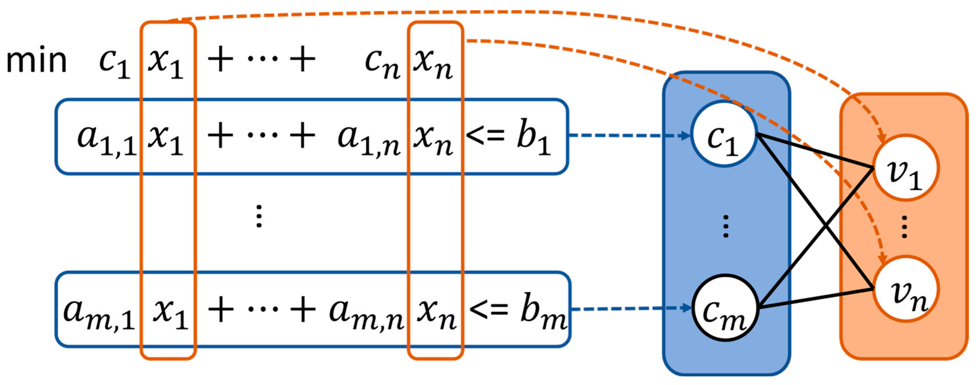
2.2. Bipartite Graph Representation for UCPs

This part describes how the UCP is transformed into a bipartite graph, a structured representation that enables GNN to learn variable–constraint interactions. Our approach adapts the MIP to the bipartite graph conversion framework proposed in [27] as shown in Figure 2.

The bipartite graph $\mathbb{G}=\left\{\mathcal{V},\mathcal{C},\mathcal{E}\right\}$ represents two disjoint sets of nodes—variables and constraints—and the edges connecting them. The associated features of these nodes and edges are summarized in

Table 1. Selected features for variables, constraints, and edges.

	Feature Description
Variables	normalized coefficient of variables in the objective function
	degree of a variable node in the bipartite representation
	average coefficient of the variable in all constraints
	maximum value among all coefficients of the variable
	minimum value among all coefficients of the variable
	whether the variable is a binary variable
	LP solution of the variable
Constraints	average of all coefficients in the constraint
	degree of constraint nodes in the bipartite representation
	right-hand-side value of the constraint
	whether the constraint is an equation constraint
Edges	coefficient value

.

• Variables: $\mathcal{V}=\left\{v_1,\dots ,v_n\right\}$, where each variable embedding $v_i\in {\mathbb{R}}^7$ corresponds to a decision variable $x_i$, partitioned as binary variables $x_1\dots x_{nb}$ (e.g., commitment, startup, and shutdown variables) and continuous variables $x_{nb+1}\dots x_n$ (e.g., power output and startup cost).
• Constraints: $\mathcal{C}=\left\{c_1,\dots ,c_m\right\}$, where each constraint embedding $c_j\in {\mathbb{R}}^4$ corresponds to the $j$-th constraint, e.g., operational rules formalized in Equations (2)–(12).
• Edges: $\left(i,j\right)\in \mathcal{E}$, which encodes the relationship where variable $x_i$ appears in constraint $b_j$ with a nonzero coefficient and has an edge embedding $e_{i,j}\in \mathbb{R}$.

2.3. Stable Binary Variables

A critical subset of binary variables in MIP exhibits persistent stability throughout the B&B process, where their values in solutions remain invariant from the root node to the final optimal solution. To systematically identify such variables, we propose a trajectory-based stability metric derived from the complete solution path of the B&B tree. Specifically, for each binary variable $x_i$, we aggregate its values across the LP relaxation solution and incumbent solutions encountered during the B&B search. The stability of $x_i$ is quantified by its normalized persistence score ${stable}_i$, which is defined as follows:

$${avg}_i={\displaystyle \frac{1}{N+1}}{\sum }_{k=0}^N{x}_i^k$$

(13)

$$stabl{e}_i=2\times \left|av{g}_i-0.5\right|$$

(14)

where $N$ is the total number of incumbent solutions during the B&B process, and $x^0$ refers to the LP relaxation solution as shown in

Table 2. Stable calculation.

Index	1	2	3	4	5	6
$x^0$	0.5	0.3	0	0	0	1
$x^1$	1	0	0	1	0	1
$x^2$	0	1	0	1	0	1
$x^3$	0	0	0	1	0	1
$x^N$	0	0	1	0	0	1
$stable$	0.4	0.48	0.6	0.2	1	1

. The stability score $stabl{e}_i$ ranges from 0 to 1, with higher values indicating a greater consistency of $x_i$.

This approach rigorously distinguishes truly stable variables from those exhibiting transient stability or noise-induced pseudo-stability. By leveraging the entire solution trajectory rather than relying on heuristic thresholds or single-node relaxations, the method ensures robustness against branching decisions and algorithmic perturbations.

3. Framework

This section presents the comprehensive framework, detailing the process from offline training of the GNN to variable fixation, initial solution setup, and ultimately obtaining the final dispatch plan. The framework is designed to enhance the efficiency and scalability of solving the UCP by leveraging data-driven insights and optimization techniques.

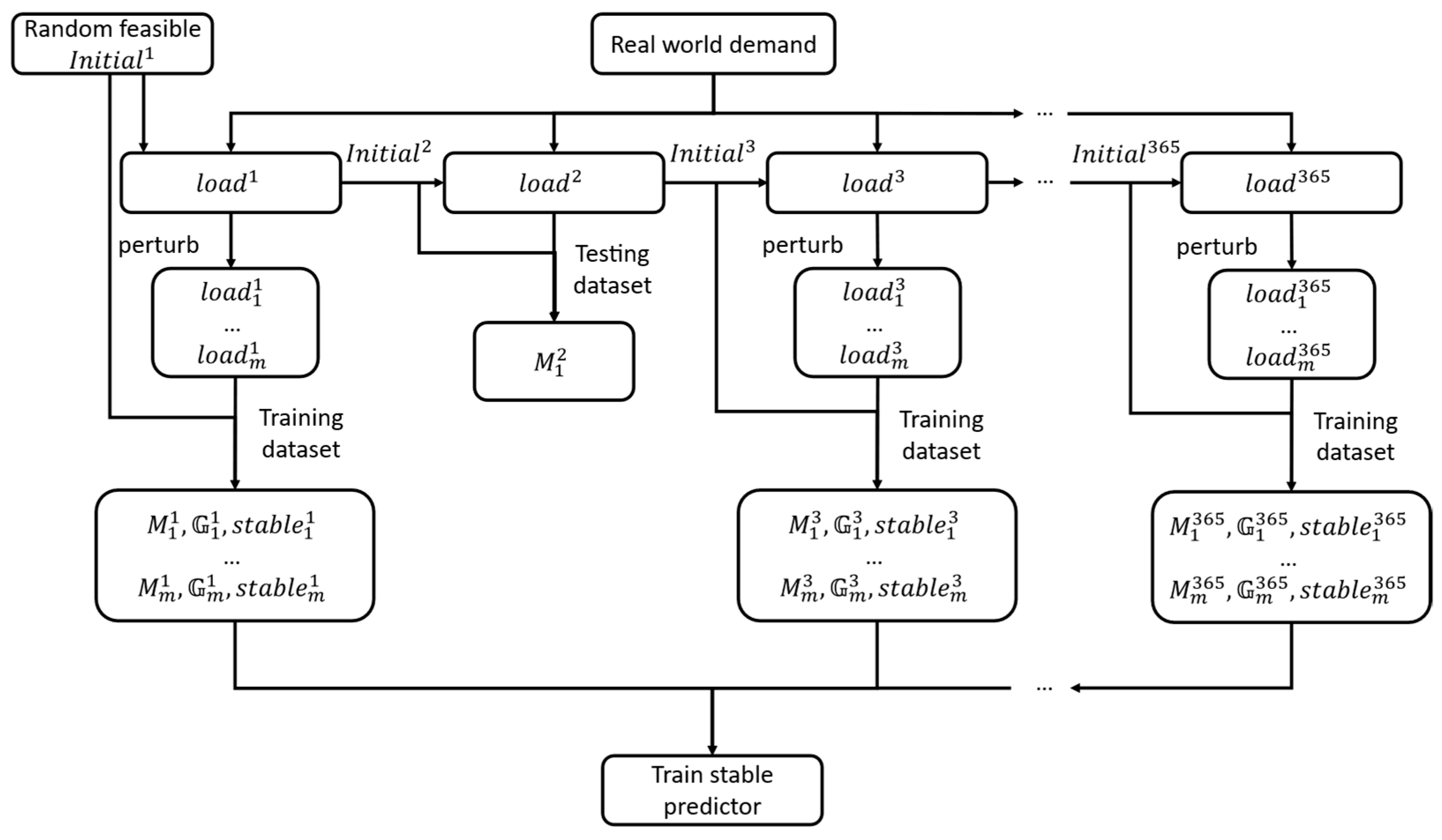
3.1. Dataset Collection

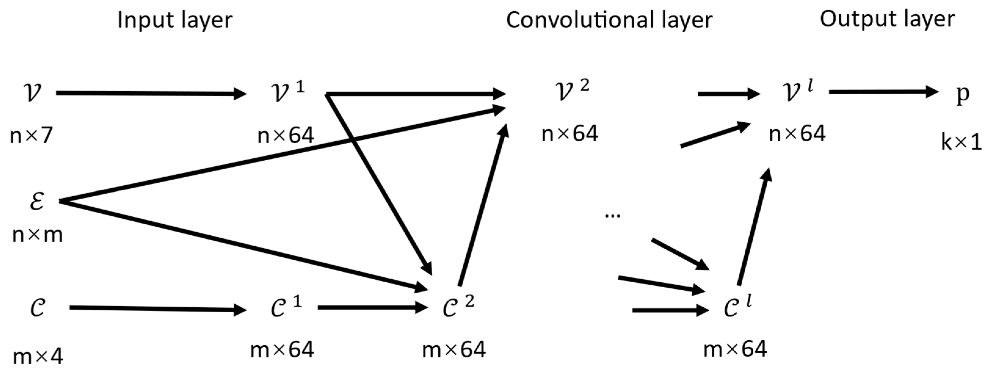
Real-world electricity demand data for an entire year are obtained and linearly scaled to match the capacity of the target power system. This scaled demand serves as the historical load profile. To avoid infeasible solutions caused by randomly initialized generator states (e.g., on/off statuses and continuous uptime/downtime), we sequentially solve the UCP for each day in the historical load profile. The final generator states (including continuous operating hours and power outputs) at the end of each day are preserved and used as the initial state for the next day. This ensures feasible and realistic transitions between instances.

Figure 3 shows how the dataset was collected. A subset of the load profiles is used as the test set, while the remaining profiles form the basis of the training set. For each training-day load, ${\mathrm{load}}^i$, we apply slight perturbations to generate multiple variations denoted as ${\mathrm{load}}_1^i,\dots ,{\mathrm{load}}_m^i$. Each perturbed load, ${\mathrm{load}}_j^i$, is paired with the same initial generator state, ${\mathrm{initial}}^i$, producing a set of UCP instances $M_1^i,\dots M_m^i$. Both the training and validation sets undergo perturbations to expand the dataset. Models trained on the training set are validated on the validation set, and the model exhibiting the best performance on the validation set is retained for testing on the test set. For the test set, instances are generated using the original training-day loads to evaluate the performance of the proposed framework in the numerical experiment section.

For each instance $M_j^i$, a bipartite graph ${\mathbb{G}}_j^i$ is constructed following the method described in Section 2.2, and its corresponding stability vector ${\mathrm{stable}}_j^i$ is calculated as described in Section 2.3. It is worth noting that it is impossible to collect all feasible solutions from the B&B search tree, so all feasible solutions explored during the solver’s process are used as a substitute.

3.2. Offline Phase

We train a bipartite GNN-based policy stable predictor ${\pi }_{\theta }$ following previous work [27], where $\pi$ denotes the policy as a function and $\theta$ represents the set of trainable parameters. The policy is designed to learn patterns from specific operational scenarios, enabling the prediction of variable stability for the UCP under unseen but similarly distributed scenarios.

$\mathcal{D}=\left\{(\mathbb{G},stable)\right\}$ denotes the training set. The policy is a three-layer structure shown in Figure 4 and is described as follows:

• Input layer: This layer, consisting of a regularization layer, fully connected layers, and activation functions, inputs the embedding ${\mathcal{V}}^0=\left\{v_1^0,\dots ,v_n^0\right\}$, ${\mathcal{C}}^0=\left\{c_1^0,\dots ,c_m^0\right\}$, where $v_i^0=v_i$, $c_j^0=c_j$ will be embedded into a higher-dimensional latent vector ${\mathcal{V}}^1$, ${\mathcal{C}}^1$.
• Convolutional layer: The information of neighboring nodes $c_j^l\in {\mathcal{C}}^l$ and $v_i^l\in {\mathcal{V}}^l$ is transitioned after a multilayer convolutional layer and takes the following form:

  $$c_j^l\leftarrow f_c(c_j^{l-1},layernorm({\sum }_i^{\left(i,j\right)\in E}{f}_{vc}(v_i^{l-1},c_j^{l-1},e_{i,j})))$$

  (15)

  $$v_i^l\leftarrow f_v(v_i^{l-1},layernorm({\sum }_j^{\left(i,j\right)\in E}{f}_{cv}(v_i^{l-1},c_j^{l-1},e_{i,j})))$$

  (16)

  where $f_c,f_v,f_{vc},f_{cv}$ are Multilayer Perceptrons with ReLU activation functions, and $layernorm$ represents the layer normalization function.
• Output layer: This layer consists of fully connected layers and a sigmoid activation function, which maps the output to a scalar in the range [0, 1], representing the stability confidence of each variable ${\pi }_{\theta }\left(\mathbb{G}\right)=\left\{p_1,\dots ,p_k\right\}$ and $p_i\in [0,1],\mathrm{i}\in \left\{1,\dots ,\mathrm{k}\right\}$. Depending on the task setting, we can selectively retain the stability predictions of specific types of binary variables—for example, only the commitment variables, or all binary variables. The remaining variables are discarded from further consideration.

Similar to the selective retention in the output layer, the training labels are also selectively clipped. Specifically, we retain only the stability indicators corresponding to certain variables as training labels, represented as $stable\in [0,1{]}^k$, while discarding the labels for the remaining variables. Given that the labels are continuous values bounded within [0, 1], the Binary Cross-Entropy (BCE) loss function is employed, which is ideally suited for such probabilistic labels. The loss function is defined as follows:

$$L\left(\theta \right)={\displaystyle \frac{-1}{\left|\mathcal{D}\right|}}\sum _{\left(\mathbb{G},stable\right)\in \mathcal{D}}\sum _{i=1}^k[stabl{e}_i\cdot \mathrm{l}\mathrm{o}\mathrm{g}\left(p_i\right)+(1-stabl{e}_i)\cdot log\left(1-p_i\right)]$$

(17)

3.3. Online Phase

This subsection presents the online phase of our optimization framework, which executes two interdependent routines during MILP solving: (1) machine learning-guided variable fixation to prune the search space and (2) machine learning-guided branching rules to prioritize critical variables. Together, these components construct a reduced model—a modified version of the original UCP model in which certain variable values are fixed and branching priorities are informed by learned patterns. This co-designed strategy significantly accelerates the solving process compared to the original UCP, especially under time-sensitive operational requirements.

3.3.1. Learning-Guided Fixing

The GNN is designed to output predictions exclusively for binary variables, where each value is constrained to the interval [0, 1] via a sigmoid activation function. These values represent stability confidence scores, with higher values indicating greater stability of the corresponding integer variable. To identify stable variables to be fixed, a dual-threshold criterion is applied. The set of binary variables $x_{g,t}$ for $x\in \left\{u,s,d\right\}$ and $\mathrm{g}\in \dot{G},\hspace{1em}\mathrm{t}\in \dot{T}$ is considered, where

• $u_{g,t}$, $s_{g,t}$, and $d_{g,t}$ represent commitment variables, startup variables, and shutdown variables of unit $g$ in time $t$;
• $\dot{G}$ and $\dot{T}$ denote the set of units and time periods, respectively.

We define a stable set ${\mathbb{S}}^{stable}$ as follows:

$${\mathbb{S}}^{stable}=\left\{(x,g,t)|x\in \left\{u,s,d\right\},\mathrm{g}\in \dot{G},\hspace{1em}\mathrm{t}\in \dot{T},{\mathbb{X}}_{g,t}^x\ge {\tau }^{stable}\wedge \left(r_{g,t}^x\le {\tau }^v\vee r_{g,t}^x\ge 1-{\tau }^v\right)\right\}$$

(18)

where

• ${\mathbb{X}}_{g,t}^x$ represents the stable predictor output (stability confidence score) for the $(g,t)$-th index and the variable type $x$;
• $r_{g,t}^x$ represents the LP relaxation value for the $(g,t)$-th index and the variable type $x$;
• ${\tau }^{stable}$ is the stability threshold, such that variables with ${\mathbb{X}}_{g,t}^x\ge {\tau }^{stable}$ are considered stable;
• ${\tau }^v$ is the integrality tolerance threshold, ensuring that $r_{g,t}^x$ is sufficiently close to a binary value.

Only variables fulfilling both conditions are provisionally classified as stable. This joint criterion ensures that stability predictions are both statistically confident and theoretically aligned with the problem’s LP relaxation properties, thereby reducing false positives caused by spurious correlations in the GNN’s latent space. The threshold parameters are tunable to balance solution quality and computational efficiency across varying UCP instances.

While fixing the generator state-transition variables $s_{g,t}$ (startup) and $d_{g,t}$ (shutdown) to 1 at specific time steps risks suboptimality due to the dynamic adjustability of power outputs, we propose a temporally flexible fixing strategy to balance solution quality and computational efficiency. Generators often exhibit flexibility in their startup/shutdown timing, and delaying or advancing commitments by several time steps may still yield feasible and near-optimal solutions. The fixation strategy can be classified into hard fix and soft fix, depending on the degree of flexibility allowed.

Rigid fixation to a single time step may exclude such solutions, while allowing a small temporal window $∆$ to preserve optimality while reducing branching. For each unit $g$ and time step $t$, the following fixation rules are applied:

• Hard fix: ${\mathbb{S}}^{hard}$ is denoted as the set of indices that are hard-fixed. These variables are forced into a fixed state, ensuring that the solution adheres to the rounded LP relaxation value for each time step. We define ${\mathbb{S}}^{hard}$ as follows:

  $${\mathbb{S}}^{hard}=\left\{\forall x\in \left\{u,s,d\},(x,g,t\right\}\in {\mathbb{S}}^{stable}|{\sum }_{j=max(0,t-∆)}^{min(T,t+∆)}{r}_{g,j}^s+r_{g,j}^d=0\right\}$$

  (19)

  For a given time $t$ of unit $g$, if all three binary variables (commitment, startup, and shutdown) are stable, and there are no startup or shutdown actions in the neighboring time steps, then these variables will be hard-fixed to their rounded LP relaxation value. It is worth noting that a partial binary solution from the rounded LP relaxation value does not guarantee feasibility.
• Soft fix: ${\mathbb{S}}^{soft}$ is denoted as the set of indices that are soft-fixed, ${\mathbb{S}}^{soft}={\mathbb{S}}^{stable}-{\mathbb{S}}^{hard}$. For variables $(x,g,t)\in {\mathbb{S}}^{soft}$, we initialize the variable to the rounded LP relaxation value but allow the solver to adjust the value during the optimization process.

3.3.2. Learning-Guided Branching

To fully leverage the GNN’s stability predictions, every integer variable in the model is assigned a customized branch priority. The stability scores generated by our GNN not only guide variable fixing but also serve as a critical indicator for divide-and-conquer strategies in B&B. Variables with low stability (close to 0) exhibit inconsistent values across nodes in the B&B tree, implying that their unresolved status contributes significantly to the solution space fragmentation. Prioritizing these variables for early branching helps accelerate bound tightening, and resolving unstable variables reduces feasible region ambiguity, enabling faster pruning of suboptimal branches.

We map stability scores ${\mathbb{X}}_{g,t}^x\in [0,1]$ to integer priorities ${\mathbb{P}}_{g,t}^x\in \left\{{\mathbb{P}}_{min},\dots ,{\mathbb{P}}_{max}\right\}$ via

$${\mathbb{P}}_{\mathrm{g},\mathrm{t}}^{\mathrm{x}}=⌊{\mathbb{P}}_{min}+\left({\mathbb{P}}_{max}-{\mathbb{P}}_{min}\right)\left(1-{\mathbb{X}}_{g,t}^x\right)⌋$$

(20)

where $⌊·⌋$ is the rounding operator to the nearest integer; ${\mathbb{P}}_{max}$ is the maximum priority; and ${\mathbb{P}}_{min}$ is the minimum priority.

In practice, this mapping can be integrated right before invoking the solver. After constructing the MIP model, we traverse each integer variable $x_{g,t}$, retrieve its predicted ${\mathbb{X}}_{g,t}^x$ from the offline-trained model, compute ${\mathbb{P}}_{\mathrm{g},\mathrm{t}}^{\mathrm{x}}$ according to the above formula, and set the corresponding branch priority in the solver. Once the branch priorities are updated, the solver will systematically prioritize branching on high-priority (low-stability) variables, the solver can more quickly prune large swathes of the search tree, leading to faster convergence in practice.

${\tau }^{stable},{\tau }^v,∆$ are set to 0.5, 0.99, and 1, respectively, in the experiments.

4. Numerical Experiments

4.1. Case Settings

The case study is performed by Gurobi 11.0 using the Python 3.11 API on a PC with an Intel Core i7-8700 CPU running at 3.20 GHz and with 32 GB of memory. All feasible solutions produced by Gurobi in the solution process are recorded.

1.

Power system setting: The three systems are taken from [10], and their sizes are reported in

Table 3. Test system summary.

Case Size	Variable	Integer	Constraint	Nonzero
50	6000	3600	10,848	50,678
100	12,000	7200	21,648	101,349
1080	129,600	77,760	233,328	1,109,492

. Each of these systems comprises solely thermal generating units.

2.

Demand setting: There are 365 loads from the first day of the year to the 365th day of the year, which are findings that come from [28]. In order to match the loads to the target systems, the loads for the 365 days, $origin loads$, are mapped to the capacity of the corresponding systems, $scaled loads$. Specifically, for each system, the upper ($sy{s}_{up}$) and lower ($sy{s}_{low}$) bounds of the target load mapping interval are determined based on the system’s maximum generation capacity scaled by factors $s_{up}$ and $s_{low}$:

$$sy{s}_{up}=\mathrm{maximum} \mathrm{generation} \mathrm{capacity}\times s_{up}$$

(21)

$$sy{s}_{low}=sy{s}_{up}\times s_{low}$$

(22)

$origin loads$ is then normalized and scaled to $scaled loads$ to fit the target system:

$$scaled loads={\displaystyle \frac{origin loads-min(origin loads)}{max(origin loads)-min(origin loads)}}\times (sy{s}_{up}-sy{s}_{low})+sy{s}_{low}$$

(23)

A simple rule is applied for dataset partitioning: days ending with the digit seven are assigned to the validation set, those ending with two are assigned to the testing set, and the remaining days are assigned to the training set. And each load will be perturbed to expand the dataset.

3.

Benchmark setting: The latest Gurobi solver 11.0 was used with the following settings: threads set to 1 and MIPGap set to 1 × 10⁻⁶. All other settings were kept at their default values.

4.2. Accuracy Comparison for Different Binary Variables

We compare the Mean Squared Error (MSE) of predictions for three types of binary variables ($u$ for commitment variables, $s$ for startup variables, and $d$ for shutdown variables) under three different system sizes (50 units, 100 units, and 1080 units), and the lower the better. As shown in

Table 4. Variable loss comparison.

Variable Type	50	100	1080
$u$	0.04773	0.02801	0.06902
$s$	0.00951	0.00765	0.02248
$d$	0.00923	0.00646	0.02100

, startup and shutdown maintain substantially lower MSE values than commitment across all system scales, indicating that GNN predicts the startup and shutdown variables with much higher accuracy than the commitment variable.

To validate the benefits of including additional variables and eliminate the influence of fixed strategies and branching strategies, we designed experiments where stable variables were simply fixed using a soft fix. Based on the selection of binary variables, the methods can be categorized into three types: only commitment variables (the approach used in most existing papers) as “M1”, only startup and shutdown variables as “M2”, or all three types of binary variables as “M3”, and we use the state-of-the-art solver Gurobi as the baseline. We use the primal gap [29] to evaluate the performance of different methods, which defined ${\displaystyle \frac{v-v^{*}}{v^{*}}}$, where $v^{*}$ is the best objective value obtained by any approach in the portfolio for comparison and $v$ is the primal bound.

Figure 5 shows the primal gap as a function of runtime. In all methods applied to the three systems, a soft fix for all three variables shows the best performance. Especially in the 100-unit system, the M3 gap exhibits the fastest decline, while the other methods take more than 100 s to reach the gap achieved by M3 in just 50 s.

4.3. Ablation Study

The effectiveness of hard fix and branching priority settings is validated, as shown in Figure 6. “M4” represents the complete fixing strategy proposed in Section 3, while “M5” denotes the comprehensive online strategy introduced in the same section, which includes both the fixing strategy and a customized branching rule. By comparing M3 and M4, it can be concluded that our proposed learning-guided fixing strategy leads to a faster initial decline in the objective function compared to using only a soft fix, especially on the 100-unit and 1080-unit systems. A comparison between M4 and M5 further demonstrates the effectiveness of the branching priority strategy on the 1080-unit system, where M5 consistently achieves an earlier reduction in the gap. However, for smaller-scale systems, adjusting the branching strategy did not have a significant impact.

5. Conclusions

This work proposes a GNN-LP hybrid learning framework to accelerate UCP optimization through stability-driven variable fixation and adaptive search strategies. Key contributions include the following:

1.

Variable Stability Classification: We design a variable fixation strategy that integrates GNN-predicted stability and LP root relaxation to guide the hard and soft fixation of binary variables. Stable variables are fixed to shrink the search space, while temporal flexibility is preserved for variables with uncertain stability. This layered fixation mechanism significantly reduces suboptimality, as confirmed by ablation studies across 50-, 100-, and 1080-unit systems.

2.

Utilization of Multi-Type Binary Variables: Instead of focusing solely on commitment variables, we incorporate startup and shutdown variables into both the MIP formulation and learning framework. These auxiliary variables enhance the stability inference of commitment variables to enable safer and more accurate hard fixation, thereby reducing suboptimality and introducing additional stable candidates for soft fixation, which accelerates the solution process by further reducing the search space. Experiments show that this joint modeling approach consistently improves primal gaps and solving times over single-variable baselines, particularly in large-scale settings.

3.

Stability-Aware Branching Prioritization: We leverage predicted variable stability to guide the branching process in branch-and-bound trajectories. By assigning a higher branching priority to unstable variables, the solver is able to explore critical decisions earlier, tighten bounds faster, and accelerate convergence. This strategy achieved faster gap reduction and earlier convergence.

While the proposed branching prioritization strategy based on variable stability has demonstrated significant efficiency gains, it remains relatively simple in its current form. Additionally, the success of incorporating auxiliary binary variables into our learning and optimization framework suggests broader applicability. Future work could investigate which types or structures of multi-variable models yield the best performance, and how such strategies can be generalized to other UCP acceleration frameworks, for example, by leveraging power system topology via graph-based representations to enhance prediction accuracy and generalization.

References

1. Anjos, M.F.; Conejo, A.J. Unit commitment in electric energy systems. Found. Trends Electr. Energy Syst. 2017, 1, 220–310. [Google Scholar] [CrossRef]
2. Hua, B.; Baldick, R.; Wang, J. Representing Operational Flexibility in Generation Expansion Planning Through Convex Relaxation of Unit Commitment. IEEE Trans. Power Syst. 2017, 33, 2272–2281. [Google Scholar] [CrossRef]
3. Ongsakul, W.; Petcharaks, N. Unit commitment by enhanced adaptive Lagrangian relaxation. IEEE Trans. Power Syst. 2004, 19, 620–628. [Google Scholar] [CrossRef]
4. Delarue, E.; Cattrysse, D.; D’Haeseleer, W. Enhanced priority list unit commitment method for power systems with a high share of renewables. Electr. Power Syst. Res. 2013, 105, 115–123. [Google Scholar] [CrossRef]
5. Hobbs, W.J.; Hermon, G.; Warner, S.; Shelbe, G.B. An enhanced dynamic programming approach for unit commitment. IEEE Trans. Power Syst. 1988, 3, 1201–1205. [Google Scholar] [CrossRef]
6. Gurobi Optimization, L. Gurobi Optimizer Reference Manual. IEEE Trans. Autom. Control 2024, 28, 1–11. [Google Scholar]
7. Ibm, L. ILOG CPLEX. Available online: http://www.ilog.com/products/cplex (accessed on 1 December 2024).
8. Bendotti, P.; Fouilhoux, P.; Rottner, C. On the complexity of the unit commitment problem. Ann. Oper. Res. 2019, 274, 119–130. [Google Scholar] [CrossRef]
9. Yang, L.; Zhang, C.; Jian, J.; Meng, K.; Xu, Y.; Dong, Z. A novel projected two-binary-variable formulation for unit commitment in power systems. Appl. Energy 2017, 187, 732–745. [Google Scholar] [CrossRef]
10. Harjunkoski, I.; Giuntoli, M.; Poland, J.; Schmitt, S. Matheuristics for Speeding Up the Solution of the Unit Commitment Problem. In Proceedings of the 2021 IEEE PES Innovative Smart Grid Technologies Europe (ISGT Europe), Espoo, Finland, 18–21 October 2021; pp. 1–5. [Google Scholar]
11. Pourahmadi, F.; Kazempour, J. Unit Commitment Predictor with a Performance Guarantee: A Support Vector Machine Classifier. IEEE Trans. Power Syst. 2024, 40, 715–727. [Google Scholar] [CrossRef]
12. Qu, S.; Yang, Z. Optimality Guaranteed UC Acceleration via Interactive Utilization of Adjoint Model. IEEE Trans. Power Syst. 2024, 39, 5191–5203. [Google Scholar] [CrossRef]
13. Sayed, A.R.; Zhang, X.; Wang, G.; Wang, Y.; Shaaban, M.; Shahidehpour, M. Deep Reinforcement Learning-Assisted Convex Programming for AC Unit Commitment and Its Variants. IEEE Trans. Power Syst. 2024, 39, 5561–5574. [Google Scholar] [CrossRef]
14. Chen, Z.; Liu, J.; Wang, X.; Yin, W. On Representing Mixed-Integer Linear Programs by Graph Neural Networks. In Proceedings of the Eleventh International Conference on Learning Representations, Kigali, Rwanda, 1–5 May 2023. [Google Scholar]
15. Schmitt, S.; Harjunkoski, I.; Giuntoli, M.; Poland, J.; Feng, X. Fast Solution of Unit Commitment Using Machine Learning Approaches. In Proceedings of the 2022 IEEE 7th International Energy Conference (ENERGYCON), Riga, Latvia, 9–12 May 2022; pp. 1–6. [Google Scholar]
16. Quan, R.; Jian, J.; Mu, Y. Tighter relaxation method for unit commitment based on second-order cone programming and valid inequalities. Int. J. Electr. Power Energy Syst. 2014, 55, 82–90. [Google Scholar] [CrossRef]
17. Ma, Z.; Zhong, H.; Xia, Q.; Kang, C.; Wang, Q.; Cao, X. A Unit Commitment Algorithm with Relaxation-Based Neighborhood Search and Improved Relaxation Inducement. IEEE Trans. Power Syst. 2020, 35, 3800–3809. [Google Scholar] [CrossRef]
18. Huang, T.; Ferber, A.; Tian, Y.; Dilkina, B.; Steiner, B. Local branching relaxation heuristics for integer linear programs. In Proceedings of the International Conference on Integration of Constraint Programming Artificial Intelligence, and Operations Research, Nice, France, 29 May–1 June 2023; pp. 96–113. [Google Scholar]
19. Gao, Q.; Yang, Z.; Li, W.; Yu, J. Optimality-Guaranteed Acceleration of Unit Commitment Calculation via Few-shot Solution Prediction. IEEE Trans. Power Syst. 2024, 40, 1583–1595. [Google Scholar] [CrossRef]
20. Pineda, S.; Morales, J.M. Is learning for the unit commitment problem a low-hanging fruit? Electr. Power Syst. Res. 2022, 207, 107851. [Google Scholar] [CrossRef]
21. Xavier, Á.S.; Qiu, F.; Ahmed, S. Learning to solve large-scale security-constrained unit commitment problems. INFORMS J. Comput. 2021, 33, 739–756. [Google Scholar] [CrossRef]
22. Yang, N.; Yang, C.; Wu, L.; Shen, X.; Jia, J.; Li, Z.; Chen, D.; Zhu, B.; Liu, S. Intelligent data-driven decision-making method for dynamic multisequence: An E-seq2seq-based SCUC expert system. IEEE Trans. Ind. Inform. 2021, 18, 3126–3137. [Google Scholar] [CrossRef]
23. Ramesh, A.V.; Li, X. Feasibility Layer Aided Machine Learning Approach for Day-Ahead Operations. IEEE Trans. Power Syst. 2024, 39, 1582–1593. [Google Scholar] [CrossRef]
24. Park, S.; Chen, W.; Han, D.; Tanneau, M.; Van Hentenryck, P. Confidence-Aware Graph Neural Networks for Learning Reliability Assessment Commitments. IEEE Trans. Power Syst. 2024, 39, 3839–3850. [Google Scholar] [CrossRef]
25. Han, Q.; Yang, L.; Chen, Q.; Zhou, X.; Zhang, D.; Wang, A.; Sun, R.; Luo, X. A GNN-Guided Predict-and-Search Framework for Mixed-Integer Linear Programming. In Proceedings of the Eleventh International Conference on Learning Representations, Kigali, Rwanda, 1–5 May 2023. [Google Scholar]
26. Qin, J.; Yu, N. Solve Large-scale Unit Commitment Problems by Physics-Informed Graph Learning. arXiv 2023, arXiv:2311.15216. [Google Scholar]
27. Gasse, M.; Chételat, D.; Ferroni, N.; Charlin, L.; Lodi, A. Exact Combinatorial Optimization with Graph Convolutional Neural Networks. arXiv 2019, arXiv:1906.01629. [Google Scholar]
28. Gridmod. RTS-GMLC: Repository for Grid Modernization Lab Consortium (GMLC) Real-Time Simulation Project. In GitHub. 2023. Available online: https://github.com/GridMod/RTS-GMLC (accessed on 1 December 2024).
29. Berthold, T. Primal Heuristics for Mixed Integer Programs. Master’s Thesis, Technische Universität, Berlin, Germany, 2006. [Google Scholar]
Figure 1. Overall framework of proposed acceleration method.
Applsci 15 04498 g001
Figure 2. Transforming a UCP formulation to a bipartite graph.
Applsci 15 04498 g002
Figure 3. Dataset flowchart.
Applsci 15 04498 g003
Figure 4. Architecture of the bipartite GNN policy π θ .
Applsci 15 04498 g004
Figure 5. The primal gap as a function of runtime, averaged over 36 instances. From left to right, the units are 50, 100, and 1080.
Applsci 15 04498 g005
Figure 6. The primal gap as a function of runtime, averaged over 36 instances. From left to right, the units are 50, 100, and 1080.
Applsci 15 04498 g006