Fuzzy Control and Modeling Techniques Based on Multidimensional Membership Functions Defined by Fuzzy Clustering Algorithms

Abstract

The increasing complexity of nonlinear multivariable systems poses significant challenges for effective modeling and control. Fuzzy modeling and control typically use fuzzy inference with one-dimensional membership functions. However, the use of multidimensional membership functions can provide significant benefits in optimizing and reducing the computational cost of a fuzzy controller. In this work, we propose the use of fuzzy clustering techniques to adjust and design multidimensional membership functions. These techniques represent a well-developed and comprehensive framework, though they are often disconnected from traditional fuzzy modeling and control methodologies. Thus, this work also seeks to combine fuzzy techniques of different applications with a single ultimate goal, namely, to optimize the modeling and control of nonlinear systems. Our main objective is system identification, modeling, and control using the Takagi–Sugeno method based on one-dimensional and multidimensional membership functions. Moreover, a comparison of various fuzzy clustering techniques for the design of multidimensional membership functions is carried out to demonstrate the effectiveness of the proposed methods in optimizing control performance and reducing computational cost.

1. Introduction

The application of fuzzy logic [1] has significantly advanced artificial intelligence by incorporating human-like uncertainty into computational decision-making. This approach has been particularly integrated in the modeling and control of nonlinear systems with the Takagi–Sugeno (T-S) fuzzy model [2]. By decomposing a complex nonlinear system into a collection of linearized subsystems interconnected through fuzzy inference, the T-S model provides a structured framework for system identification and control. Recent studies [3,4,5] have explored and extended the capabilities of T-S fuzzy models in recent years.

The approach developed in [6] can be considered as a generalized version of the T-S method. This technique is designed to be computationally efficient, realizing enhanced model accuracy on the basis of parameter weighting. In [7], the method was further developed to accommodate multivariable systems. Compared to the original T-S model [2], these approaches demonstrate high accuracy in modeling nonlinear systems.

On the other hand, the authors of [8] introduced an enhanced T-S fuzzy modeling approach that uses multidimensional membership functions (MDMFs) to improve system identification. Their method eliminates a limitation of the conventional fuzzy inference method based on 1DMFs that can lead to suboptimal placement of fuzzy rules when modeling nonlinear multivariable systems. In contrast, the adoption of MDMFs enhances system identification while requiring fewer fuzzy rules. A genetic algorithm (GA) is integrated to optimize the MDMFs in combination with the T-S approach for modeling and system identification. Experimental results demonstrate that this method achieves lower identification errors compared to the traditional T-S model while reducing the number of fuzzy rules.

Despite advances in the use of MDMFs in fuzzy models, their application in nonlinear multivariable systems remains limited. One major limitation is the challenge of properly tuning membership functions in complex systems, which can lead to reduced accuracy of system identification and control. In this paper, we address this gap by proposing an approach based on MDMFs defined through fuzzy clustering algorithms.

Other algorithms have been developed to facilitate this task, such as the one proposed in [9], which optimizes the placement of MDMFs using a new algorithm based on the inertia matrix. In [10], collaborative fuzzy clustering (CFC) was applied to the identification of multiple-input multiple-output (MIMO) systems.

Different adjustment algorithms have been explored through several methods in order to determine the parameters of MDMFs (antecedents) and the T-S model (consequents). One such approach is the application of GAs [8,11,12]; in this approach, the GA is used for optimizing the T-S antecedents and the T-S identification method [2] is used to estimate the consequents.

In addition to the optimization of MDMFs, fuzzy clustering algorithms have been developed to obtain fuzzy rules for the best separation of data in clustering problems. Examples of these algorithms are fuzzy C-means (FCM) [13,14,15], fuzzy possibilistic c-means [16], Gustafson–Kessel (GK) [17,18,19], Gath–Geva (GG) [20], and other approaches [21].

The K-means approach to clustering was initially proposed by S. Lloyd in 1957 [22] as a technique for modulation via coded impulses. However, it was James MacQueen [23] who finished defining it and assigned the current name ten years later. The fuzzy K-means clustering algorithm was created by J. Bezkek and his team [24], who developed it in 1984.

In 1978, Gustafson and Kessel [17] proposed a fuzzy clustering algorithm with fuzzy covariances. This algorithm can better estimate the precision of mixed densities.

In 1989, Gath and Geva presented their own fuzzy clustering algorithm, which aims to perform fuzzy clustering without a priori knowledge of the number of clusters necessary to classify the set of samples. The validity of membership in these clusters is based on performance measures using the criteria of hypervolume and density [25].

In [26], the authors proposed a fuzzy-based controller for sink selection and clustering in wireless sensor networks. Their proposed method considers the capacity of sink nodes to optimize data transmission and prevent packet loss. Furthermore, a fuzzy-based controller is designed to select cluster heads by reducing the number of fuzzy rules using the R-implications method, which decreases the complexity and energy consumption of the system. Simulation results demonstrate that this approach enhances network lifetime, reduces packet loss, and improves energy efficiency compared to traditional clustering techniques.

In [27], an anti-swing control method for overhead crane systems was developed by integrating the clustering salp swarm algorithm (CSSA) with a fuzzy PID controller. The proposed approach enhances population diversity and improves convergence accuracy by introducing clustering techniques into the original salp swarm algorithm (SSA). Similarly, a fuzzy control approach based on the extraction and reduction of fuzzy rules through the FCM clustering algorithm was presented in [28]. This method optimizes a self-tuning fuzzy proportional–derivative controller by reducing the number of fuzzy rules while maintaining control accuracy. The authors demonstrated the effectiveness of these approaches through simulation experiments, showing superior performance compared to conventional fuzzy and PID controllers in mitigating overhead crane oscillations along with improved control precision.

A fuzzy tuning approach for the controller parameters of a parallel manipulator based on clustering analysis was proposed in [29]. The new technique improves tracking performance throughout the robot workspace by identifying specific configurations that represent different levels of load inertia. Using the FCM clustering algorithm, inertial data are classified and representative cluster centers are determined to enable efficient tuning of the controller parameters for arbitrary configurations. The results obtained from a prototype demonstrate the effectiveness of this methodology in improving control quality without requiring complex real-time computations.

The authors of [30] presented a hybrid approach combining a fuzzy logic controller (FLC) and FCM to enhance the asset management of power transformers. Their proposed methodology provides diagnoses and prognoses of incipient power transformer faults using a system that incorporates critical parameters such as dissolved gas analysis, interfacial tension, etc. Their study used a dataset consisting of 200 transformer tests for verification, demonstrating that the fuzzy clustering approach can effectively classify insulation conditions into four clusters ranging from healthy insulation to insulation that is nearing the end of its useful life.

In [31] the authors demonstrated target recognition capability in remote sensing images acquired by a small UAV using fuzzy clustering techniques. To facilitate improved object detection and localization, the fuzzy clustering algorithm was applied to construct an intelligent target recognition model that effectively segments and classifies remote sensing data. The performance of the proposed system was verified through simulation experiments, demonstrating its effectiveness and robustness.

In [32], the authors proposed a fuzzy control framework for aircraft engines by integrating dynamic clustering modeling with robust control strategies. Their approach utilizes a hierarchical clustering technique to optimize the number of fuzzy rules, ensuring accurate representation of the engine’s dynamic behavior while maintaining computational efficiency. Experimental verification through hardware-in-the-loop (HIL) tests demonstrated the effectiveness of the proposed model, achieving improved engine performance with reduced settling times and overshoots.

In another method presented in [33], the authors introduced an advanced clustering-based fuzzy segmentation technique for medical image processing, specifically brain magnetic resonance imaging (MRI) segmentation. By incorporating spatial constraints and local membership matrix information, the proposed algorithm enhances traditional fuzzy C-means (FCM) clustering to achieve greater noise resistance and segmentation accuracy.

In this work, different fuzzy clustering techniques are considered, allowing for the construction of clusters with undetermined limits. These methods allow a specific sample to belong to several different clusters, with the respective relationships determined by degrees of membership.

In other words, the main essence of fuzzy clustering is not only to consider the membership of a sample in a certain cluster, but to consider the degree to which it belongs to each of the clusters obtained in the application. The latter represents a great advantage when it comes to representing all the complexity that a set of samples can offer in a real data collection.

Additionally, we evaluate the advantages that fuzzy clustering methodologies can provide in the context of control engineering. Our aim is to obtain a more effective controller by classifying samples of the system to be controlled.

The main contributions of this paper can be summarized as follows:

• Development of a novel method for identifying and controlling nonlinear systems using MDMFs.
• Integration of fuzzy clustering algorithms to optimize the generation of MDMFs, leading to a reduced number of fuzzy rules while maintaining model accuracy.
• A demonstration of the effectiveness of the proposed approach using the example of a thermal mixing tank system.

The rest of this paper is structured as follows: Section 2 provides a brief description of the T-S identification method based on 1DMFs inference; Section 3 presents fuzzy control based on multidimensional membership functions, where these functions are adjusted by fuzzy clustering algorithms; finally, Section 4, uses an illustrative example of a thermal mixing tank system to demonstrate the advantages of our proposed fuzzy clustering methods over traditional fuzzy approaches.

2. T-S Identification Method

The identification methodology for T-S fuzzy models is formulated as an optimization problem in which the nonlinear system parameters are estimated by minimizing a quadratic performance index [2]. However, the conventional T-S identification approach becomes ineffective when triangular membership functions overlap in pairs, leading to a T-S matrix that is rank-deficient and consequently non-invertible [6]. To overcome this limitation, a generalized T-S identification framework incorporating a parameter weighting strategy was proposed in [6,7] to enhance the robustness of the estimation process.

The above method is based on the identification of nonlinear functions that can be expressed as a set of difference equations by the following IF–THEN rules for an nth order system:

$$\begin{array}{cc}\hfill S^{(i_1\cdots i_m)}& :\mathrm{If} z_1\left(k\right) \mathrm{is} M_1^{i_1} \mathrm{and} \dots \mathrm{and} z_m\left(k\right) \mathrm{is} M_m^{i_m} \mathrm{then}:\hfill \\ \hfill y_i(k+1)& =a_{i0}^{(i_1\cdots i_m)}+a_{i1}^{(i_1\cdots i_m)}{y}_i\left(k\right)+\cdots +a_{i{n}_i}^{(i_1\cdots i_m)}{y}_i(k-n_i+1)+\hfill \\ \hfill & +\sum _{j=1}^p{b}_{ij1}^{(i_1\cdots i_m)}{u}_j\left(k\right)+\cdots +b_{ij{n}_i}^{(i_1\cdots i_m)}{u}_j(k-n_i+1)\hfill \end{array}$$

(1)

where $\left\{y_1\left(k\right),y_2\left(k\right),\dots y_s\left(k\right)\right\}$ are the system outputs, $\left\{u_1\left(k\right),u_2\left(k\right),\dots u_p\left(k\right)\right\}$ are the system inputs, and $\left\{z_1\left(k\right),z_2\left(k\right),\dots z_m\left(k\right)\right\}$ are measurable variables, hereinafter referred to as fuzzy variables. The term $S^{(i_1\dots i_m)}$ denotes the $(i_1\dots i_m)$th fuzzy rule, while the parameters $a_{i0\dots i{n}_i}^{(i_1\dots i_m)}$ and $b_{ij1\dots ij{n}_i}^{(i_1\dots i_m)}$ are coefficients associated with the output and input values, respectively.

In this fuzzy framework, j designates the fuzzy variable index and $i_j$ denotes the fuzzy rule index associated with the corresponding fuzzy variable. Under this denotation, the fuzzy estimation of the output is provided by

$$\begin{array}{cc}\hfill & {\widehat{y}}_i(k+1)=\sum _{i_1=1}^{r_1}\cdots \sum _{i_m=1}^{r_m}{\beta }^{(i_1\dots i_m)}\left(z_{(i_1\dots i_m)}\left(k\right)\right)\left[a_{i0}^{(i_1\dots i_m)}+a_{i1}^{(i_1\dots i_m)}{y}_i\left(k\right)+\cdots +\right.\hfill \\ \hfill & +a_{i{n}_i}^{(i_1\dots i_m)}{y}_i(k-n_i+1)+\sum _{j=1}^p\left.b_{ij1}^{(i_1\dots i_m)}{u}_j\left(k\right)+\cdots +b_{ij{n}_i}^{(i_1\dots i_m)}{u}_j(k-n_i+1)\right],\hfill \end{array}$$

(2)

where

$${\beta }^{(i_1\dots i_m)}\left(z_{(i_1\dots i_m)}\left(k\right)\right)={\displaystyle \frac{{\prod }_{j=1}^m\left({\mu }_{j{i}_j}\left(z_j\left(k\right)\right)\right)}{{\sum }_{i_1=1}^{r_1}\cdots {\sum }_{i_m=1}^{r_m}\left({\prod }_{j=1}^m\left({\mu }_{j{i}_j}\left(z_j\left(k\right)\right)\right)\right)}},$$

(3)

in which ${\mu }_{j{i}_j}\left(z_j\right)$ represents the membership function associated with the fuzzy set $M_j^{i_j}$. In the context of the parameter weighting method, it is assumed that an initial affine linear estimation model is available, i.e., that a preliminary estimation of the following parameters is known:

$$P_0=\left[\begin{array}{cccccccccc}{a}_{i0}^0& \cdots & a_{i{n}_i}^0& b_{i11}^0& \cdots & b_{i1n_i}^0& \cdots & b_{ip1}^0& \cdots & b_{ip{n}_i}^0\end{array}\right].$$

(4)

To obtain this first estimation, the classical least squares method can be applied to the set of data in the system. This estimation can then be utilized as reference parameters for all the T-S fuzzy model subsystems:

$$\begin{array}{c}\hfill p_0=\underset{r_1·r_2\cdots r_m}{\underbrace{{\left[\begin{array}{cccc}{P}_0& P_0& \cdots & P_0\end{array}\right]}^t}}.\end{array}$$

(5)

Then, the fuzzy model parameters can be obtained by minimizing

$$\begin{array}{cc}\hfill & J=\sum _{k=1}^{n_s}{\left(y\left(k\right)-\widehat{y}\left(k\right)\right)}^2+{\gamma }^2\sum _{i_1=1}^{r_1}\cdots \sum _{i_m=1}^{r_m}\sum _{j=0}^n{\left(p_j^0-p_j^{(i_1\dots i_m)}\right)}^2=\hfill \\ \hfill & ={∥Y-XP∥}^2+{\gamma }^2{∥p_0-P∥}^2={∥\left[\begin{array}{c}Y\\ \gamma p_0\end{array}\right]-\left[\begin{array}{c}X\\ \gamma I\end{array}\right]P∥}^2={∥Y_a-X_{a}P∥}^2,\hfill \end{array}$$

(6)

where Y represents the output data, X represents the fuzzy input/output data, and P stands for the parameters of the fuzzy model.

As explained in [6,7], the matrix $X^{t}X$ is non-invertible due to the linear dependency among the columns of X, which makes direct computation of the parameter vector P via the classical expression $P={\left(X^{t}X\right)}^{(-1)}{X}^{t}Y$ infeasible. To overcome this limitation, a factor $\gamma$ is introduced. This parameter quantifies the confidence degree associated with the initially estimated parameters; its inclusion ensures that the extended matrix $X_a$ maintains full rank even if the triangular membership functions overlap in pairs. Thus, the vector P can be determined by isolating it from Equation (6):

$$\begin{array}{cc}\hfill & J={∥Y_a-X_{a}P∥}^2={(Y_a-X_{a}P)}^t(Y_a-X_{a}P)\hfill \\ \hfill & \nabla J=X_a^t(Y_a-X_{a}P)=X_a^t{Y}_a-X_a^t{X}_{a}P=0\hfill \\ \hfill & P={\left(X_a^t{X}_a\right)}^{-1}{X}_a^t{Y}_a.\hfill \end{array}$$

(7)

In the case where the state variables are measurable [7], Equation (1) can also be represented by a set of discrete state-space models:

$$\begin{array}{cc}\hfill S^{(i_1\dots i_m)}& : \mathrm{If} z_1\left(k\right) \mathrm{is} M_1^{i_1} \mathrm{and} \dots \mathrm{and} z_m\left(k\right) \mathrm{is} M_m^{i_m}, \mathrm{then}:\hfill \\ \hfill x(k+1)& =a_0^{(i_1\dots i_m)}+A^{(i_1\dots i_m)}x\left(k\right)+B^{(i_1\dots i_m)}u\left(k\right).\hfill \end{array}$$

(8)

Thus, fuzzy identification can be accomplished with state models [7] using similar formulations to Equations (2) and (3).

Note that in the T-S identification method the fuzzy rules weights $w^{(i_1\dots i_m)}={\prod }_{j=1}^m\left({\mu }_{j{i}_j}\left(z_j\right)\right)$ are inherently determined by the inference of 1DMFs ${\mu }_{j{i}_j}\left(z_j\right)$. In this work, we propose MDMFs to solve this problem.

3. Fuzzy Control Based on Multidimensional Membership Functions Adjusted by Fuzzy Clustering Algorithms

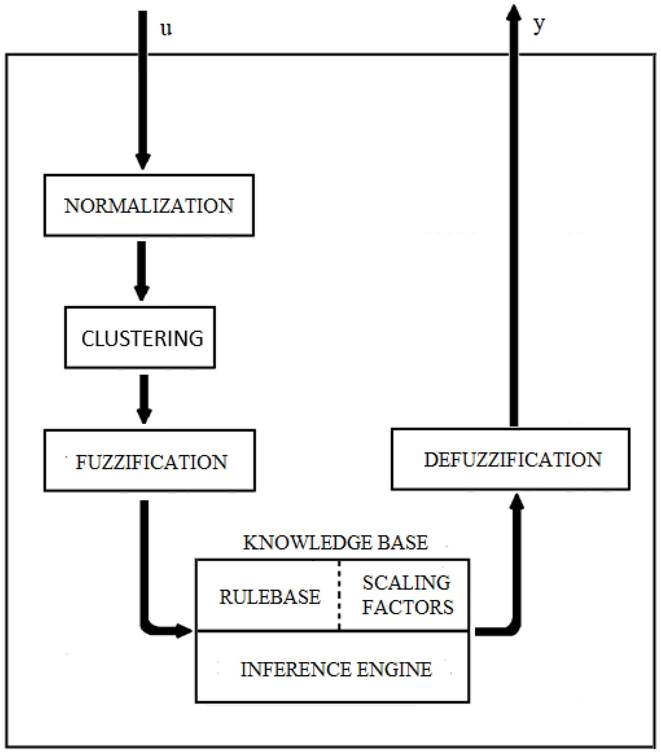
This work presents a new method that for the identification, modeling, and control of nonlinear systems described by the T-S model. The proposed method uses MDMFs and different clustering methods to adjust these functions, achieve a better fit of these functions, and even reduce the number of membership functions necessary to achieve adequate control of the nonlinear system. Figure 1 shows the control process using clustering techniques, illustrating the basic structure of a fuzzy system.

The approach proposed in this work for multidimensional fuzzy sets $M_i$ is described below. The fuzzy variable is defined as follows:

$$\begin{array}{cc}\hfill z& ={\left[\begin{array}{cccc}{z}_1& z_2& \cdots & z_f\end{array}\right]}^t\hfill \\ \hfill z& \in {\mathbb{R}}^f\hfill \end{array}$$

(9)

and the MDMF is defined as ${\mu }_i\left(z\right)$. For each multidimensional fuzzy set, a central point $z_iϵ{\mathbb{R}}^f$ must be designed. This central point is defined by clustering methods in order to select points that produce a greater separation between the datasets. In this work, the dataset used for the clustering process corresponds to the set of measured input–output samples collected from the system under study.

The concept of distance should also be defined, as there are several ways to define it [34]. The distance is needed in order to establish the proximity of a certain sample with respect to the central points of the membership functions, which is related to the degree of membership regarding each of the rules. Clustering techniques further determine and define this distance depending on which technique was selected during the design phase. In addition, the multidimensional membership rules are determined based on the clustering method and the parameters chosen to calculate them. Thus, the form of these membership rules changes according to the methodology used.

The fuzzy model of the system with $n_r$ rules is represented as follows:

$$\begin{array}{cc}\hfill S^i& : \mathrm{If} z\left(k\right) \mathrm{is} M^i \mathrm{then}:\hfill \\ \hfill y_1(k+1)& =a_{10}^i+a_{11}^i{y}_1\left(k\right)+\cdots +a_{1n_1}^i{y}_1(k-n_1+1)+\hfill \\ \hfill & +\sum _{j=1}^p{b}_{1j1}^i{u}_j\left(k\right)+\cdots +b_{1j{n}_1}^i{u}_j(k-n_1+1),\hfill \end{array}$$

(10)

which becomes

$$\begin{array}{cc}\hfill {\widehat{y}}_1(k+1)& =\sum _{i=1}^{n_r}{\alpha }_i\left(z\left(k\right)\right)\left[a_{10}^i+a_{11}^i{y}_i\left(k\right)+\cdots +a_{1n_1}^i{y}_1(k-n_1+1)+\right.\hfill \\ \hfill & +\sum _{j=1}^p\left.b_{1j1}^i{u}_j\left(k\right)+\cdots +b_{1j{n}_1}^i{u}_j(k-n_1+1)\right],\hfill \end{array}$$

(11)

where

$${\alpha }_i\left(z\left(k\right)\right)={\displaystyle \frac{{\mu }_i\left(z\left(k\right)\right)}{{\sum }_{i=1}^{n_r}{\mu }_i\left(z\left(k\right)\right)}}.$$

(12)

To obtain a fuzzy controller based on MDMFs, it is possible to design a controller and observer for each fuzzy rule using any controller and observer design methodology that meets the desired robustness, precision, and speed conditions. In this work, the incremental state model is used [35], as it has the advantage of introducing an integral action, which in turn allows a steady-state error of zero to be maintained in fuzzy T-S control based on MDMFs. The discrete LQR method and the optimal state observer are also applied, as defined in [35]. Nonlinear systems can be treated using the T-S fuzzy model based on MDMFs when the multidimensional fuzzy variable is known $z={\left[\begin{array}{cccc}{z}_1& z_2& \cdots & z_f\end{array}\right]}^t$.

Recalling the fuzzy model of the system with $n_r$ rules previously presented in (10), the difference equation associated with each output can be transformed into a state model with an affine term, as follows:

$$\begin{array}{cc}\hfill & x_1(k+1)=\left[\begin{array}{c}{a}_{10}·a_{11}\\ a_{10}·a_{12}\\ ⋮\\ a_{10}·a_{1n}\end{array}\right]+\left[\begin{array}{ccccc}{a}_{11}& 1& 0& \cdots & 0\\ a_{12}& 0& 1& \cdots & 0\\ ⋮& ⋮& \ddots & \ddots & ⋮\\ a_{1n}& 0& \cdots & 0& 1\end{array}\right]x_i\left(k\right)\hfill \\ \hfill & +\left[\begin{array}{cccc}{b}_{111}& b_{121}& \cdots & b_{1p1}\\ b_{112}& b_{122}& \cdots & b_{1p2}\\ ⋮& ⋮& \ddots & ⋮\\ b_{11n}& b_{12n}& \cdots & b_{1pn}\end{array}\right]\left[\begin{array}{c}{u}_1\left(k\right)\\ u_2\left(k\right)\\ ⋮\\ u_p\left(k\right)\end{array}\right]\hfill \\ \hfill & y_1\left(k\right)=a_{10}+\left[\begin{array}{cccc}1& 0& \cdots & 0\end{array}\right]x_1\left(k\right).\hfill \end{array}$$

(13)

This means that

$$\begin{array}{cc}\hfill & x_1(k+1)=x_{10}+A_1{x}_1\left(k\right)+B_{1}u\left(k\right)\hfill \\ \hfill & y_1\left(k\right)=a_{10}+C_1{x}_1\left(k\right),\hfill \end{array}$$

(14)

where $A_1\in {\mathbb{R}}^{n\times n}$, $B_1\in {\mathbb{R}}^{n\times p}$, and $C_1\in {\mathbb{R}}^{s\times n}$.

Grouping the whole system in a unique model, the following equation is obtained:

$$\begin{array}{c}\hfill \left[\begin{array}{c}{x}_1(k+1)\\ x_2(k+1)\\ ⋮\\ x_s(k+1)\end{array}\right]=\left[\begin{array}{c}{x}_{10}\\ x_{20}\\ ⋮\\ x_{s0}\end{array}\right]+\left[\begin{array}{cccc}{A}_1& 0& \cdots & 0\\ 0& A_2& \ddots & 0\\ ⋮& \ddots & \ddots & ⋮\\ 0& 0& \cdots & A_s\end{array}\right]\left[\begin{array}{c}{x}_1\left(k\right)\\ x_2\left(k\right)\\ ⋮\\ x_s\left(k\right)\end{array}\right]+\left[\begin{array}{c}{B}_1\\ B_2\\ ⋮\\ B_s\end{array}\right]\left[\begin{array}{c}{u}_1\left(k\right)\\ u_2\left(k\right)\\ ⋮\\ u_p\left(k\right)\end{array}\right]\\ \hfill \left[\begin{array}{c}{y}_1\left(k\right)\\ y_2\left(k\right)\\ ⋮\\ y_s\left(k\right)\end{array}\right]=\left[\begin{array}{c}{a}_{10}\\ a_{20}\\ ⋮\\ a_{s0}\end{array}\right]+\left[\begin{array}{cccc}{C}_1& 0& \cdots & 0\\ 0& C_2& \ddots & 0\\ ⋮& \ddots & \ddots & ⋮\\ 0& 0& \cdots & C_s\end{array}\right]\left[\begin{array}{c}{x}_1\left(k\right)\\ x_2\left(k\right)\\ ⋮\\ x_s\left(k\right)\end{array}\right]\end{array}$$

(15)

which can be represented as follows:

$$\begin{array}{cc}\hfill & x(k+1)=a_x+Ax\left(k\right)+Bu\left(k\right)\hfill \\ \hfill & y\left(k\right)=a_y+Cx\left(k\right).\hfill \end{array}$$

(16)

Then, the multivariate state model with independent terms and $n_r$ rules is represented as follows:

$$\begin{array}{cc}\hfill S^i& : \mathrm{If} z\left(k\right) \mathrm{is} M^i \mathrm{then}:\hfill \\ \hfill x(k+1)& =a_x^i+A^{i}x\left(k\right)+B^{i}u\left(k\right)\hfill \\ \hfill y\left(k\right)& =a_y^i+C^{i}x\left(k\right).\hfill \end{array}$$

(17)

Furthermore, the following incremental state model can be obtained in each fuzzy rule [35]:

$$\begin{array}{cc}\hfill S^i: \mathrm{If} z\left(k\right) \mathrm{is}& M^i \mathrm{then}:\hfill \\ \hfill \left[\begin{array}{c}y(k+1)\\ \delta x(k+1)\end{array}\right]& =\left[\begin{array}{cc}I& C^{i)}{A}^i\\ 0& A^i\end{array}\right]\left[\begin{array}{c}y\left(k\right)\\ \delta x\left(k\right)\end{array}\right]+\left[\begin{array}{c}{C}^i{B}^i\\ B^i\end{array}\right]\delta u\left(k\right)\hfill \\ \hfill y\left(k\right)& =\left[\begin{array}{cc}I& 0\end{array}\right]\left[\begin{array}{c}y\left(k\right)\\ \delta x\left(k\right)\end{array}\right]\hfill \\ \hfill & ⋮\hfill \end{array}$$

(18)

Next, a discrete LQR method for the fuzzy incremental state based on MDMFs is applied. For each rule, we seek to minimize the following cost index J based on the incremental state fuzzy matrices:

$$\begin{array}{c}\hfill J=\sum _{k=0}^{\infty }{\left(x_a\left(k\right)-x_{ar}\right)}^{T}Q\left(x_a\left(k\right)-x_{ar}\right)+\delta u^T\left(k\right)R\delta u\left(k\right)\end{array}$$

(19)

where the $Q\in {\mathbb{R}}^{\left(q+n\right)x\left(q+n\right)}$ and $R\in {\mathbb{R}}^{\left(pxp\right)}$ matrices must be symmetric and positive definite [6].

The fuzzy controller based on MDMFs is defined as follows:

$$\begin{array}{cc}\hfill S^i& : \mathrm{If} z\left(k\right) \mathrm{is} M^i \mathrm{then}\Delta u\left(k\right)=K^i(x_{ar}-x_a\left(k\right)).\hfill \end{array}$$

(20)

The control action is

$$u\left(k\right)=u\left(k-1\right)+\delta u\left(k\right).$$

(21)

Because the state $\mathsf{\Delta }x\left(k\right)$ is not usually accessible, a fuzzy state observer is needed:

$$\begin{array}{cc}\hfill S^i& : \mathrm{If} z\left(k\right) \mathrm{is} M^i, \mathrm{then}:\hfill \\ \hfill & x_e\left(k+1\right)=a_x^i+A^i{x}_e\left(k\right)+B^{i}u\left(k\right)+H^i(y\left(k\right)-\left({a_y}^i+C^i{x}_e\left(k\right))\right).\hfill \end{array}$$

(22)

Calculation of the observation matrix H proceeds in the same way as in [35] for each fuzzy rule defined by MDMFs, using the following optimal observer:

$$\begin{array}{cc}\hfill S^i& : \mathrm{If} z\left(k\right)\mathrm{is} M^i\mathrm{then} H^i=A^i{C^i}^T.\hfill \end{array}$$

(23)

Estimation of the incremental state can be obtained by means of the state observer shown in (24). Estimation of the state [35] is shown in (25):

$$\delta x_e=x_e\left(k\right)-x_e(k-1)$$

(24)

$$x_{ae}=\left[\begin{array}{c}{y}_k\\ \delta x_e\end{array}\right].$$

(25)

3.1. Fuzzy Clustering

Initially, a set of n samples $X=[x_1,x_2,\cdots ,x_n]$ and a number K of clusters is used. In this way, a fuzzy cluster is considered as a fuzzy subset in X, defined as shown below:

$${\mu }_k:X\to \left[0,1\right],k=1,\cdots ,K.$$

The degree of fuzzy membership for each cluster k is represented as follows:

$$u_{ik}={\mu }_k\left(x_i\right),i=1,\cdots ,nk=1,\cdots ,K.$$

(26)

In this way, $u_{ik}$ shows the degree of membership of a sample i with respect to a cluster k. In general, $u_{ik}$ satisfies the conditions provided in (27):

$$u_{ik}\in \left[0,1\right],\forall i,k;\sum _{k=1}^K{u}_{ik}=1,\forall i.$$

(27)

The results of applying a fuzzy clustering methodology are collected in a partition matrix U = ${(u}_{ik})$ that shows all the degrees of membership of the samples with respect to each cluster [36]. To calculate this matrix, the concept of distance to the centers of the clusters is applied, which depends exclusively on the fuzzy clustering method being used.

3.1.1. FCM Clustering Algorithm

The FCM algorithm [24] is based on the minimization of a cost index, described in (28):

$$J\left(X,U,V\right)=\sum _{i=1}^c\sum _{k=1}^N{\left(u_{ik}\right)}^m{∥x_k-v_i∥}^2$$

(28)

where

$$V=\left[v_1,v_2,\cdots ,v_c\right],v_i\in {\mathbb{R}}^n$$

(29)

is a vector of cluster prototypes (more commonly known as centers), which have to be obtained through the algorithm. Here, D is the norm of the squared distance of the inner product, as described in (30):

$$D_{ikA}^2={∥x_k-v_i∥}^2={\left(x_k-v_i\right)}^{T}A(x_k-v_i).$$

(30)

Statistically, (30) can be viewed as a measure of the total variance of $x_k$ from $v_i$. The minimization of this equation represents a nonlinear optimization problem that can be solved using a wide variety of methods, from minimization of grouped coordinates to the use of genetic algorithms. The most popular method is a Picard iteration through the first-order conditions for stationary points, also known as the FCM algorithm.

The stationary points can be found using Lagrange multipliers ${\Lambda }_k$, as provided in (31):

$$\overline{J}\left(X,U,V,\lambda \right)=\sum _{i=1}^c\sum _{k=1}^N{\left(u_{ik}\right)}^m{D}_{ikA}^2+\sum _{k=1}^N{\lambda }_k\left(\sum _{i=1}^c{u}_{ik}-1\right).$$

(31)

Next, the gradients of $\overline{J}$ with respect to U, V, and $\lambda$ must be set to zero. If $D_{ikA}^2>0,\forall i,k$ and m > 1, then $(U,V)\in M_{fc}x{\mathbb{R}}^{nxc}$ can minimize (32) only if (32) and (33) hold:

$$u_{ik}={\displaystyle \frac{1}{{\sum }_{j=1}^c({D_{ikA}/D_{jkA})}^{2/(m-1)}}},1\le i\le c,1\le k\le N$$

(32)

$$v_i={\displaystyle \frac{{\sum }_{k=1}^N{u}_{ik}^m{x}_k}{{\sum }_{k=1}^N{u}_{ik}^m}}1\le i\le c.$$

(33)

The FCM algorithm uses the standard Euclidean norm as a distance, meaning that clusters take the form of hyperspheres. Therefore, it can only detect clusters with the same shape and orientation, as the common choice of the norm-inducing matrix is either $A=I$ or can be chosen an $n\times n$ diagonal matrix that contains the different variances in the direction of the coordinate axes of X, as shown in (34):

$$A_D=\left[\begin{array}{ccc}{\left({\displaystyle \frac{1}{{\sigma }_1}}\right)}^2& 0& \begin{array}{cc}\cdots & 0\end{array}\\ 0& {\left({\displaystyle \frac{1}{{\sigma }_2}}\right)}^2& \begin{array}{cc}\cdots & 0\end{array}\\ \begin{array}{c}⋮\\ 0\end{array}& \begin{array}{c}⋮\\ 0\end{array}& \begin{array}{cc}\begin{array}{c}\ddots \\ \cdots \end{array}& \begin{array}{c}⋮\\ {\left({\displaystyle \frac{1}{{\sigma }_n}}\right)}^2\end{array}\end{array}\end{array}\right].$$

(34)

Additionally, A can be defined as the inverse matrix of the $n\times n$ covariance matrix, $A=F^{-1}$, with F defined in (35):

$$F={\displaystyle \frac{1}{N}}\sum _{k=1}^N(x_k-\widehat{x})(x_k-{\widehat{x})}^T.$$

(35)

In the simulations developed in Section 4, the direct application of this algorithm could induce errors in the case of multidimensional systems.

In order to avoid this problem, the data must be normalized before applying this algorithm. In this way, the distances to the center of the clusters are relative and the distances on the axis of the dimensions with a lower range of values are not neglected. Normalization of the data is carried out as shown in (36):

$$X_{norm}={\displaystyle \frac{X-\widehat{X}}{{\sigma }_X}}.$$

(36)

After the data have been normalized and the algorithm has been applied, the centers of the clusters must be denormalized, as the FCM algorithm will not have the previously normalized data.

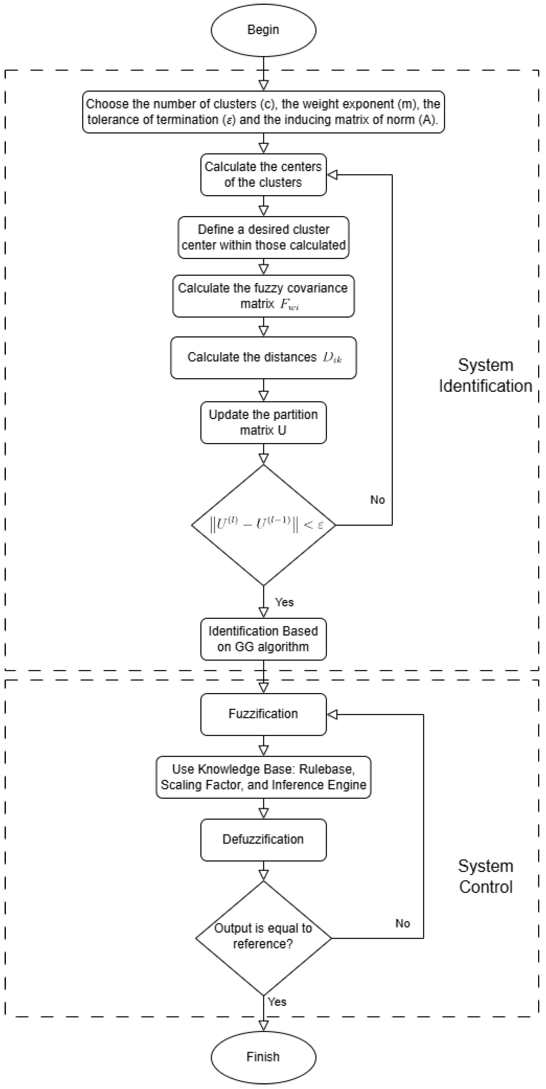
The FCM algorithm used in this work is shown in Figure 2, and is defined as follows.

-

Step 1: Given a dataset X, choose the number of clusters 1 < c < N, the weight exponent m > 1, the tolerance of termination $\epsilon >0$, and the inducing matrix of norm A. Initialize the partition matrix randomly such that ${\mathsf{U}}^{\left(0\right)}$ has arbitrary values.

-

Step 2: Normalize the data to avoid errors due to differences in the ranges of the different dimensions.

-

Step 3: Calculate the centers of the clusters such that:

$$v_i^{\left(l\right)}={\displaystyle \frac{{\sum }_{k=1}^N{u}_{ik}^{(l-1)}{x}_k}{{\sum }_{k=1}^N{u}_{ik}^{(l-1)}}}1\le i\le c,$$

(37)

where l is the current iteration number of the algorithm.

-

Step 4: Define a desired cluster center within the calculated centers in order to force its value. This center will be the same in all iterations.

-

Step 5: Calculate the distances of the samples to the centers of the clusters such that:

$$D_{ikA}^2={∥x_k-v_i∥}^2={\left(x_k-v_i\right)}^{T}A\left(x_k-v_i\right),1\le i\le c,1\le k\le N.$$

(38)

-

Step 6: Update the partition matrix U such that

$$u_{ik}={\displaystyle \frac{1}{{\sum }_{j=1}^c({D_{ikA}/D_{jkA})}^{\frac{2}{m-1}}}}.$$

(39)

-

Step 7: Repeat steps 3, 4, 5, and 6 for $l=1,2,\cdots$ until fulfilling

$$∥U^{\left(l\right)}-U^{(l-1)}∥<\epsilon .$$

(40)

-

Step 8: Denormalize the obtained cluster centers in order to properly place them within the ranges of the different dimensions.

After the centers have been obtained using the algorithm, it is necessary to include fuzzification based on the FCM formulas for the T-S and fuzzy controller identification stages. The fuzzification process for each sample is as follows:

$$\begin{array}{cc}\hfill X_n\left(k\right)& ={\displaystyle \frac{x\left(k\right)-\widehat{X}}{{\sigma }_X}}\hfill \\ \hfill D_i^2\left(k\right)={∥x_n\left(k\right)-v_i∥}^2& ={\left(x_n\left(k\right)-v_i\right)}^{T}A\left(x_n\left(k\right)-v_i\right),1\le i\le c\hfill \\ \hfill {\mu }_i\left(k\right)& ={\displaystyle \frac{1}{{\sum }_{j=1}^c{(D_i\left(k\right)/D_j\left(k\right))}^{\frac{2}{m-1}}}}.\hfill \end{array}$$

(41)

3.1.2. Fuzzy GK Clustering Algorithm

The standard FCM algorithm was extended by Gustafson and Kessel (GK) [17] by employing an adaptive norm distance, with the aim of detecting clusters of different geometric shapes within a dataset. In this way, each cluster has its own norm-inducing matrix ${\mathrm{A}}_i$ that produces its own inner product norm, as shown in (42):

$$D_{ikA}^2={\left(x_k-v_i\right)}^T{A}_i\left(x_k-v_i\right),1\le i\le c,1\le k\le N.$$

(42)

The matrices $A_i$ are used as optimization variables, and allow each cluster to adapt the distance to the topological structure of the data. The objective function of the GK algorithm is defined by (43):

$$J\left(X,U,V,A\right)=\sum _{i=1}^c\sum _{k=1}^N{u}_{ik}^m{D}_{ik{A}_i}^2.$$

(43)

However, this equation cannot be minimized directly with respect to ${\mathsf{A}}_i$, as it is linear in ${\mathsf{A}}_i$. This means that J can be made as small as desired simply by making ${\mathsf{A}}_i$ less positive definite. To obtain a feasible solution, ${\mathsf{A}}_i$ must be somehow bounded. To optimize the shape of the cluster while keeping its volume constant, we can vary the determinant of the matrix ${\mathsf{A}}_i$ such that

$$∥{\mathrm{A}}_i∥={\rho }_i,\rho >0,$$

(44)

where ${\rho }_i$ is adjusted for each cluster. Using the Lagrange multiplier method, we obtain

$${\mathrm{A}}_i={\left[{\rho }_i\det \left(F_i\right)\right]}^{{\displaystyle \frac{1}{n}}}{F}_i^{-1},$$

(45)

where $F_i$ is the fuzzy covariance matrix in cluster i, defined in (46)

$$F_i={\displaystyle \frac{{\sum }_{k=1}^N{u}_{ik}^m\left(x_k-v_i\right){\left(x_k-v_i\right)}^T}{{\sum }_{k=1}^N{u}_{ik}^m}}.$$

(46)

Note that substituting (45) and (46) into (42) provides a distance determined by the quadratic norm between ${\mathsf{x}}_k$ and the cluster center ${\mathsf{v}}_i$, where the covariance is determined by the degrees of membership in U.

The fuzzy GK clustering algorithm is outlined in Figure 3, which provides a structured flowchart of its main stages. The individual steps are as follows.

-

Step 1: Given a dataset X, choose the number of 1 < c < N clusters, the weight exponent m > 1, the termination tolerance $\epsilon >0$, and the norm inducing matrix A. Initialize the partition matrix randomly such that ${\mathsf{U}}^{\left(0\right)}$ has arbitrary values.

-

Step 2: Calculate the cluster centers as specified below, where l is the number of the current iteration of the algorithm.

$$v_i^{\left(l\right)}={\displaystyle \frac{{\sum }_{k=1}^N{{(u}_{ik}^{(l-1)})}^m{x}_k}{{\sum }_{k=1}^N{{(u}_{ik}^{(l-1)})}^m}}1\le i\le c.$$

(47)

-

Step 3: Determine one of the obtained centers as the chosen center. This center will be the same in all iterations.

-

Step 4: Calculate the covariance matrix of the clusters such that

$$F_i^{\left(l\right)}={\displaystyle \frac{{\sum }_{k=1}^N{\left(u_{ik}^{(l-1)}\right)}^m\left(x_k-v_i^l\right){\left(x_k-v_i^l\right)}^T}{{\sum }_{k=1}^N{\left(u_{ik}^{(l-1)}\right)}^m}},1\le i\le c.$$

(48)

-

Step 5: Add a scaled identity matrix

$$F_i=\left(1-\gamma \right)F_i+\gamma {\left(F_0\right)}^{{\displaystyle \frac{1}{n}}}I.$$

(49)

-

Step 6: Extract the eigenvalues ${\lambda }_{ij}$ and eigenvectors ${\varphi }_{ij}$, find ${\lambda }_{i,max}={max}_j{\lambda }_{ij}$, and set

$${\lambda }_{i,max}={\displaystyle \frac{{\lambda }_{ij}}{\beta }},\forall jforwhich{\lambda }_{i,max}/{\lambda }_{ij}\ge \beta .$$

(50)

-

Step 7: Reconstruct $F_i$ with the following form:

$$F_i=\left[\begin{array}{ccc}{\varphi }_{i1}& \cdots & {\varphi }_{in}\end{array}\right]{diag({\lambda }_{i1},\dots ,{\lambda }_{in})\left[\begin{array}{ccc}{\varphi }_{i1}& \cdots & {\varphi }_{in}\end{array}\right]}^{-1}.$$

(51)

-

Step 8: Calculate the distances

$$D_{ikA}^2={\left(x_k-v_i^{\left(l\right)}\right)}^T\left[{\left({\rho }_i\det \left(F_i\right)\right)}^{1/n}{F}_i^{-1}\right]\left(x_k-v_i^{\left(l\right)}\right).$$

(52)

-

Step 9: Update the partition matrix U as follows:

$$u_{ik}={\displaystyle \frac{1}{{\sum }_{j=1}^c{(D_{ikA}(x_k,v_i)/D_{jkA}(x_k,v_j))}^{\frac{2}{m-1}}}},1\le i\le c,1\le k\le N.$$

(53)

-

Step 10: Repeat the above steps until fulfilling

$$∥U^{\left(l\right)}-U^{(l-1)}∥<\epsilon .$$

(54)

After the centers and the covariance matrix F have been obtained by the algorithm, it is necessary to include a fuzzification based on the GK formulas for the T-S identification and fuzzy controller stages. The fuzzification process for each sample proceeds as follows:

$$D_i^2\left(k\right)={\left(x\left(k\right)-v_i\right)}^T\left[{\left({\rho }_i\det \left(F_i\right)\right)}^{1/n}{F}_i^{-1}\right]\left(x\left(k\right)-v_i\right)$$

(55)

$${\mu }_i\left(k\right)={\displaystyle \frac{1}{{\sum }_{j=1}^c{(D_i(x\left(k\right),v_i)/D_j(x\left(k\right),v_j))}^{\frac{2}{m-1}}}},1\le i\le c.$$

(56)

3.1.3. Fuzzy Clustering GG Algorithm

The fuzzy clustering of maximum likelihood estimates (FMLE) algorithm employs the fuzzy maximum likelihood estimation-based rule as the distance [25], as follows:

$$D_{ik}\left({\mathit{x}}_k,{\mathit{v}}_i\right)={\displaystyle \frac{\sqrt{\det \left(F_{wi}\right)}}{{\alpha }_i}}exp\left({\displaystyle \frac{1}{2}}{\left({\mathit{x}}_k,{\mathit{v}}_i^{\left(l\right)}\right)}^T{F}_{wi}^{-1}\left({\mathit{x}}_k,{\mathit{v}}_i^{\left(l\right)}\right)\right).$$

(57)

Note that unlike the GK algorithm, this distance involves an exponential term, meaning that it decreases faster than the induced product norm. Here, $F_{wi}$ describes the fuzzy covariance matrix in cluster i, the calculation of which is shown in (58):

$$F_{wi}={\displaystyle \frac{{\sum }_{k=1}^N{\left(u_{ik}\right)}^w\left({\mathbf{x}}_k-{\mathbf{v}}_i\right){\left({\mathbf{x}}_k-{\mathbf{v}}_i\right)}^T}{{\sum }_{k=1}^N{\left(u_{ik}\right)}^w}},1\le i\le c.$$

(58)

The degrees of membership $u_{ik}$ are interpreted as the a posteriori probability of selecting cluster i given sample $x_k$. Gath and Geva determined in their research [25] that the FMLE algorithm is capable of determining clusters of different shapes, sizes, and densities. The covariance matrix of the cluster is used in conjunction with an exponential distance, and the clusters are not constrained by their volume. However, this algorithm is much less robust, requiring a good initialization. Depending on the exponential distance, it can become unstable and provide erroneous results or alternatively converge to a near-optimal local point.

The use of a central fuzzy rule to determine a desirable working point has been considered in the same way as in common fuzzy clustering methods. The GG algorithm [25] used in this work is summarized below and illustrated in the flowchart shown in Figure 4.

-

Step 1: Given a dataset X, choose the number of 1 < c < N clusters, the weight exponent m > 1, and the termination tolerance $\epsilon >0$. Initialize the partition matrix U using a robust method.

-

Step 2: Calculate the cluster centers as follows, where l is the current iteration number of the algorithm:

$$v_i^{\left(l\right)}={\displaystyle \frac{{\sum }_{k=1}^N{(u_{ik}^{(l-1)})}^w{x}_k}{{\sum }_{k=1}^N{(u_{ik}^{(l-1)})}^w}}1\le i\le c.$$

(59)

-

Step 3: Set one of the obtained clusters as the desired fuzzy rule. This center will be the same in all iterations.

-

Step 4: Calculate the fuzzy covariance matrix of the cluster:

$$F_{wi}={\displaystyle \frac{{\sum }_{k=1}^N{\left(u_{ik}\right)}^w\left(x_k-v_i\right){\left(x_k-v_i\right)}^T}{{\sum }_{k=1}^N{\left(u_{ik}\right)}^w}},1\le i\le c.$$

(60)

-

Step 5: Calculate the distances $D_{ik}$ in the following form:

$$D_{ik}^2\left(x_k,v_i\right)={\displaystyle \frac{{\left(2\pi \right)}^{\frac{n}{2}}\sqrt{\det \left(F_{wi}\right)}}{{\alpha }_i}}exp\left({\displaystyle \frac{1}{2}}{\left(x_k,v_i^{\left(l\right)}\right)}^T{F}_{wi}^{-1}\left(x_k,v_i^{\left(l\right)}\right)\right).$$

(61)

with the following a priori probability:

$${\alpha }_i={\displaystyle \frac{1}{N}}{\sum }_{k=1}^N{u}_{ik}.$$

(62)

-

Step 6: Update the partition matrix U with the terms

$$u_{ik}={\displaystyle \frac{1}{{\sum }_{j=1}^c{(D_{ikA}(x_k,v_i)/D_{jkA}(x_k,v_j))}^{\frac{2}{m-1}}}},1\le i\le c,1\le k\le N.$$

(63)

-

Step 7: Repeat the above steps until fulfilling

$$∥U^{\left(l\right)}-U^{(l-1)}∥<\epsilon .$$

(64)

After obtaining the centers, covariance matrix F, and a priori probability $\alpha$ using algorithm, it is necessary to include a fuzzification based on the GG formulae for the T-S identification and fuzzy controller stages. The fuzzification process for each sample is as follows:

$$\begin{array}{cc}\hfill D_i^2\left(x\left(k\right),v_i\right)& ={\displaystyle \frac{{\left(2\pi \right)}^{\frac{n}{2}}\sqrt{\det \left(F_{wi}\right)}}{{\alpha }_i}}exp\left({\displaystyle \frac{1}{2}}{\left(x\left(k\right),v_i\right)}^T{F}_{wi}^{-1}\left(x\left(k\right),v_i\right)\right)\hfill \\ \hfill {\mu }_i\left(k\right)& ={\displaystyle \frac{1}{{\sum }_{j=1}^c{(D_i(x\left(k\right),v_i)/D_j(x\left(k\right),v_j))}^{\frac{2}{m-1}}}},1\le i\le c\hfill \end{array}$$

(65)

4. Thermal Mixing Tank System

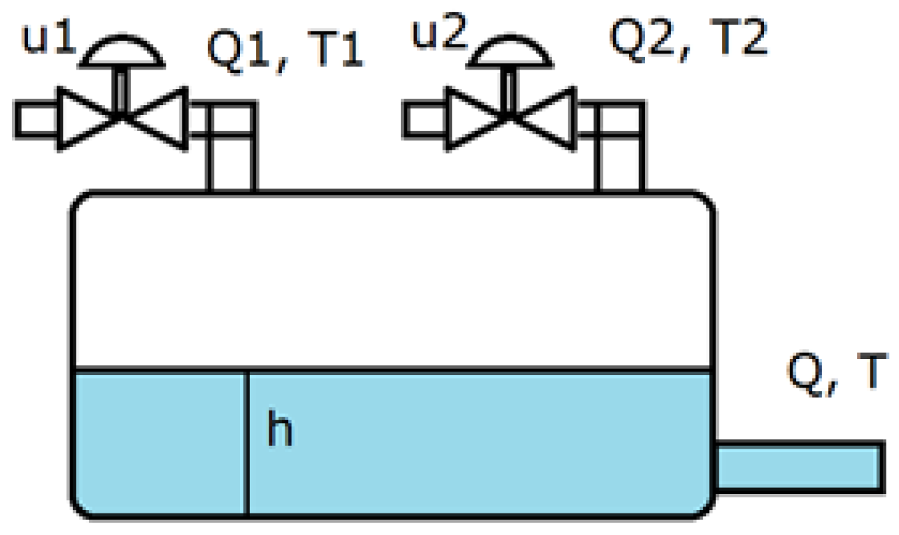
In order to check the effectiveness of each of the methods developed in this work, we investigated the modeling, identification, and control of a thermal mixing tank system consisting of a tank, two fluid inlets with different flow rates and temperatures, and a water outlet.

The studied system is multivariable and nonlinear with a pure time delay, allowing this example to show the advantages and disadvantages of the different methods mentioned above. However, it should be noted that these methods can be applied to any multivariable nonlinear system.

The thermal mixing tank is shown in Figure 5. The inlet pipes allow for the flow of fluids at two different fixed temperatures (${\mathsf{T}}_1$, ${\mathsf{T}}_2$), and their flow rates (${\mathsf{Q}}_1$, ${\mathsf{Q}}_2$) can be adjusted by opening or closing two valves (${\mathsf{u}}_1$, ${\mathsf{u}}_2$). The flow rate and outlet temperature (${\mathsf{Q}}_S$, ${\mathsf{T}}_S$) depend on the inertia of the system and the energy and mass flow of the inlet pipes. The simplified dynamic model representing the inlet flow rates is provided in (66):

$$\begin{array}{cc}\hfill Q_1\left(s\right)& ={\displaystyle \frac{K_1}{s+p_1}}{e}^{-{\tau }_{1}s}{U}_1\left(s\right)\hfill \\ \hfill Q_2\left(s\right)& ={\displaystyle \frac{K_2}{s+p_2}}{e}^{-{\tau }_{2}s}{U}_2\left(s\right).\hfill \end{array}$$

(66)

Additionally, due to the location and technology of the flow meter, a delay in the reading of the outflow is considered such that only the flow $Q_m$ in the outflow pipe can be measured, which represents the measured flow delayed by ${\tau }_S$ with respect to the outflow. The relationship between these two signals is described in (67):

$$Q_m\left(s\right)=Q_S(t-{\tau }_S).$$

(67)

Furthermore, thermal losses proportional to the temperature difference between the inside ${\mathsf{T}}_S$ and outside ${\mathsf{T}}_e$ of the mixing tank are modeled, which acts as a disturbance of the system. The dynamic model is represented by (68)

$$\begin{array}{cc}\hfill Q_1+Q_2-Q_S& =A{\displaystyle \frac{dh}{dt}}\hfill \\ \hfill T_1{Q}_1+T_2{Q}_2-{T_{S}Q}_S+& k_p(T_S-T_e)=A{\displaystyle \frac{dTh}{dt}}\hfill \\ \hfill Q_S& =\alpha \sqrt{h},\hfill \end{array}$$

(68)

where h is the tank fluid height, $K_1$ is the gain of the dynamic system of the inlet flow ${\mathsf{Q}}_1$, ${\mathsf{K}}_2$ is the gain of the dynamic system of the input flow ${\mathsf{Q}}_2$, ${\mathsf{p}}_1$ is the pole of the dynamic system of the inlet flow ${\mathsf{Q}}_1$, ${\mathsf{p}}_2$ is the pole of the dynamic system of the inlet flow rate ${\mathsf{Q}}_2$, $\alpha$ is the discharge coefficient of the outflow ${\mathsf{Q}}_S$, ${\tau }_1$ is the pure delay of the inlet flow ${\mathsf{Q}}_1$, ${\tau }_2$ is the pure delay of the inlet flow ${\mathsf{Q}}_2$, ${\tau }_S$ is the pure delay of the outflow measurement ${\mathsf{Q}}_m$, A is the cross-sectional area of the tank, ${\mathsf{K}}_p$ is the discharge coefficient of the outlet flow Q, ${\mathsf{u}}_1$ is the opening range of valve 1, and ${\mathsf{u}}_2$ is the opening range of valve 2.

In order to obtain an open-loop dataset of the system, we carried out a simulation covering long period of time during which random signals were introduced in both input variables ${\mathsf{u}}_1$ and ${\mathsf{u}}_2$ in such a way that the largest range of operation of the nonlinear system was covered.

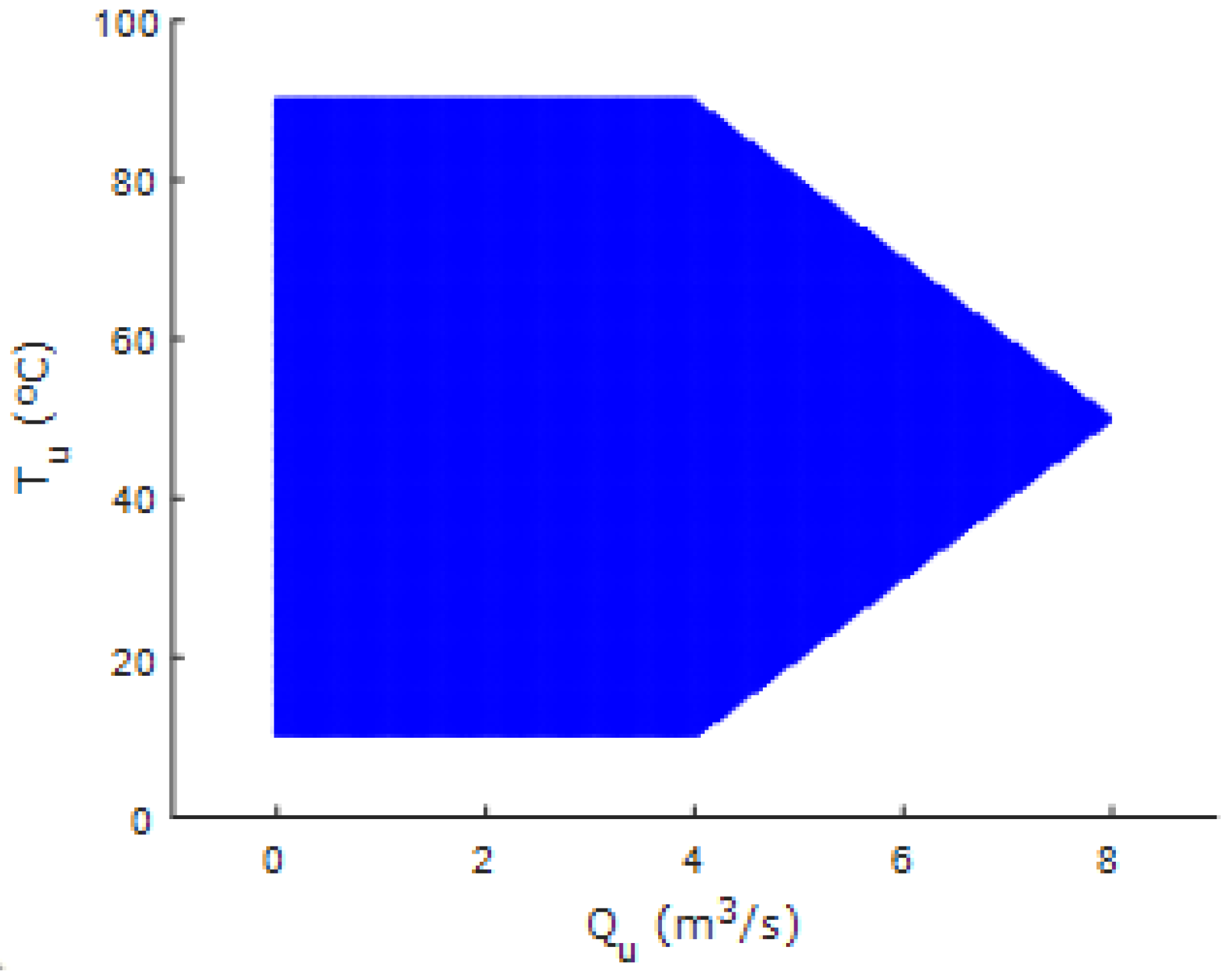
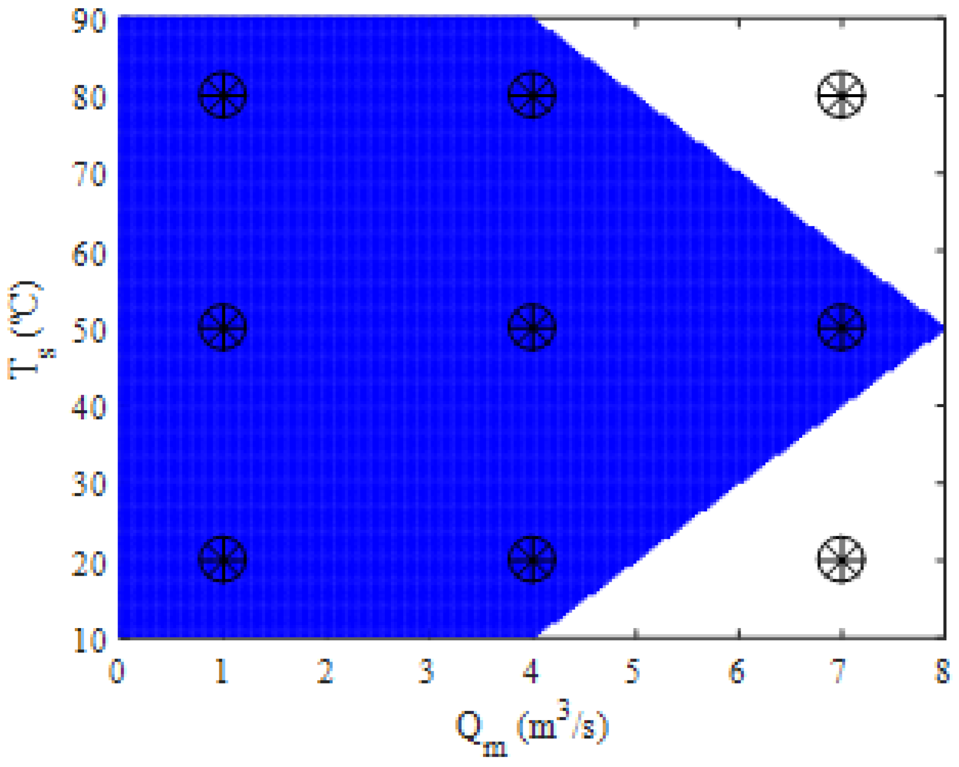
A sampling time of 0.5 s was chosen for the simulation. Figure 6 shows the temperature versus the output flow rate. As can be seen, the working range area is between 10–90 ° for the temperature and 0–7 ${\mathsf{m}}^3$/s for the flow rate.

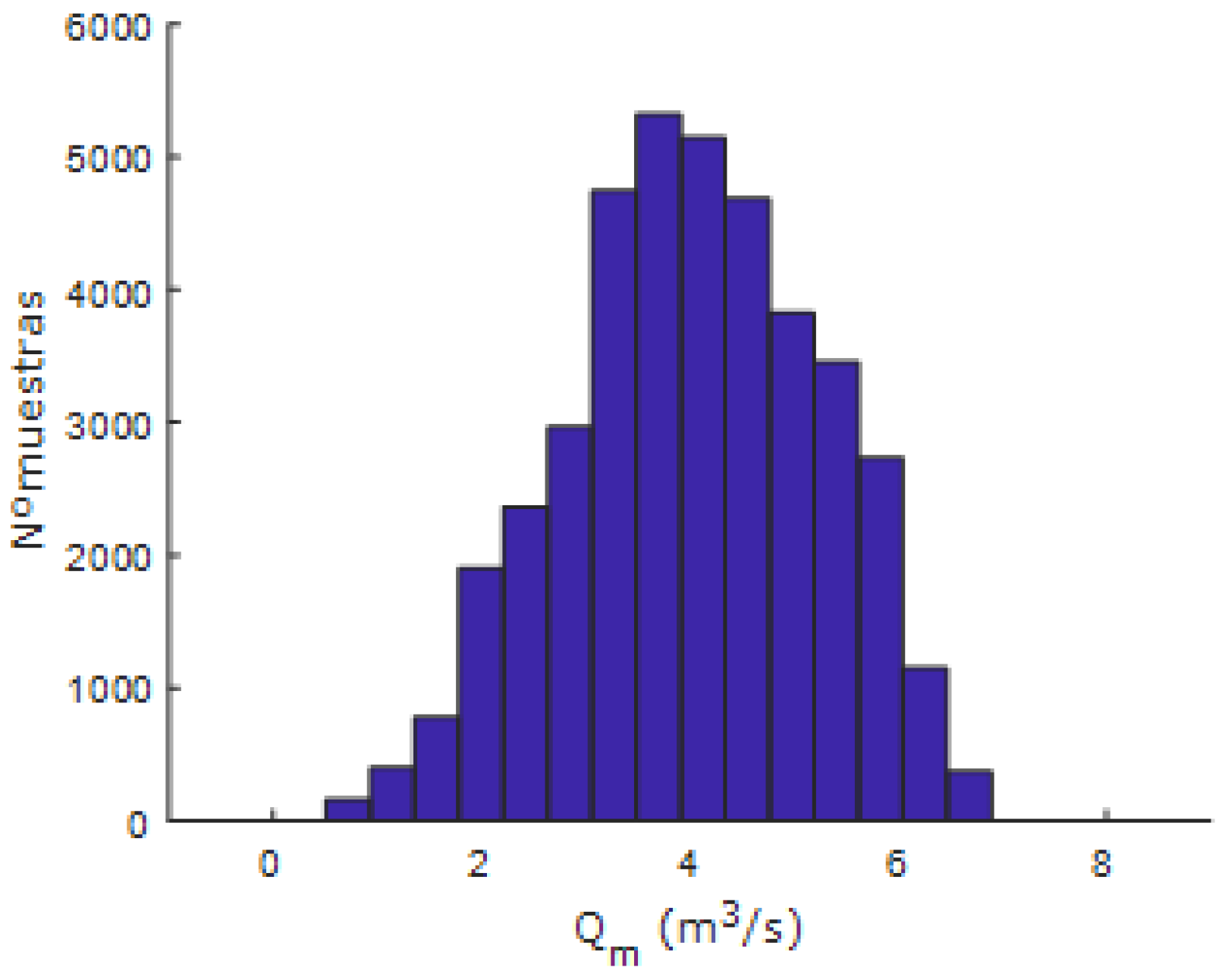
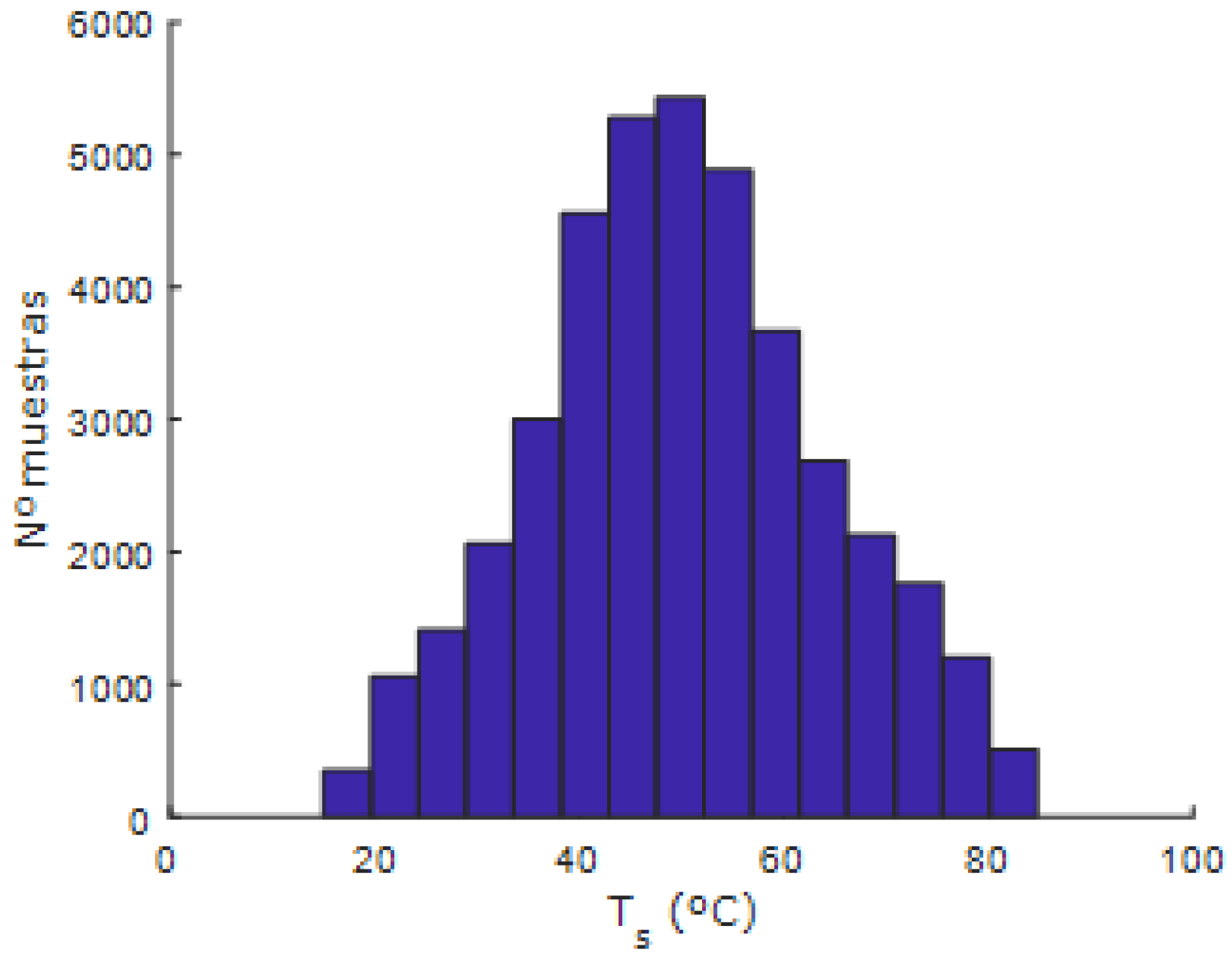
Figure 7 and Figure 8 represent the histograms of the temperature and flow rate samples of the simulated data, respectively. It can be seen from these histograms that the working range of the thermal mixing tank system is covered, with a higher concentration of data around the central area, which is the desired nominal operating point.

Uniformly distributed data were generated in order to calculate fuzzy clusters that are not affected by the accumulation of data in any particular area and that cover the entire workspace independently of the data obtained through the open-loop system simulation. These data, called uniform data, were artificially originated by covering the entire workspace area of the thermal mixing tank, and were spaced a very small distance apart. The representation of these uniform data is shown in Figure 9.

4.1. Fuzzy Modeling and Control Based on One-Dimensional Membership Functions

First, the modeling, identification, and fuzzy control based on one-dimensional membership functions is established, as detailed in Section 2.

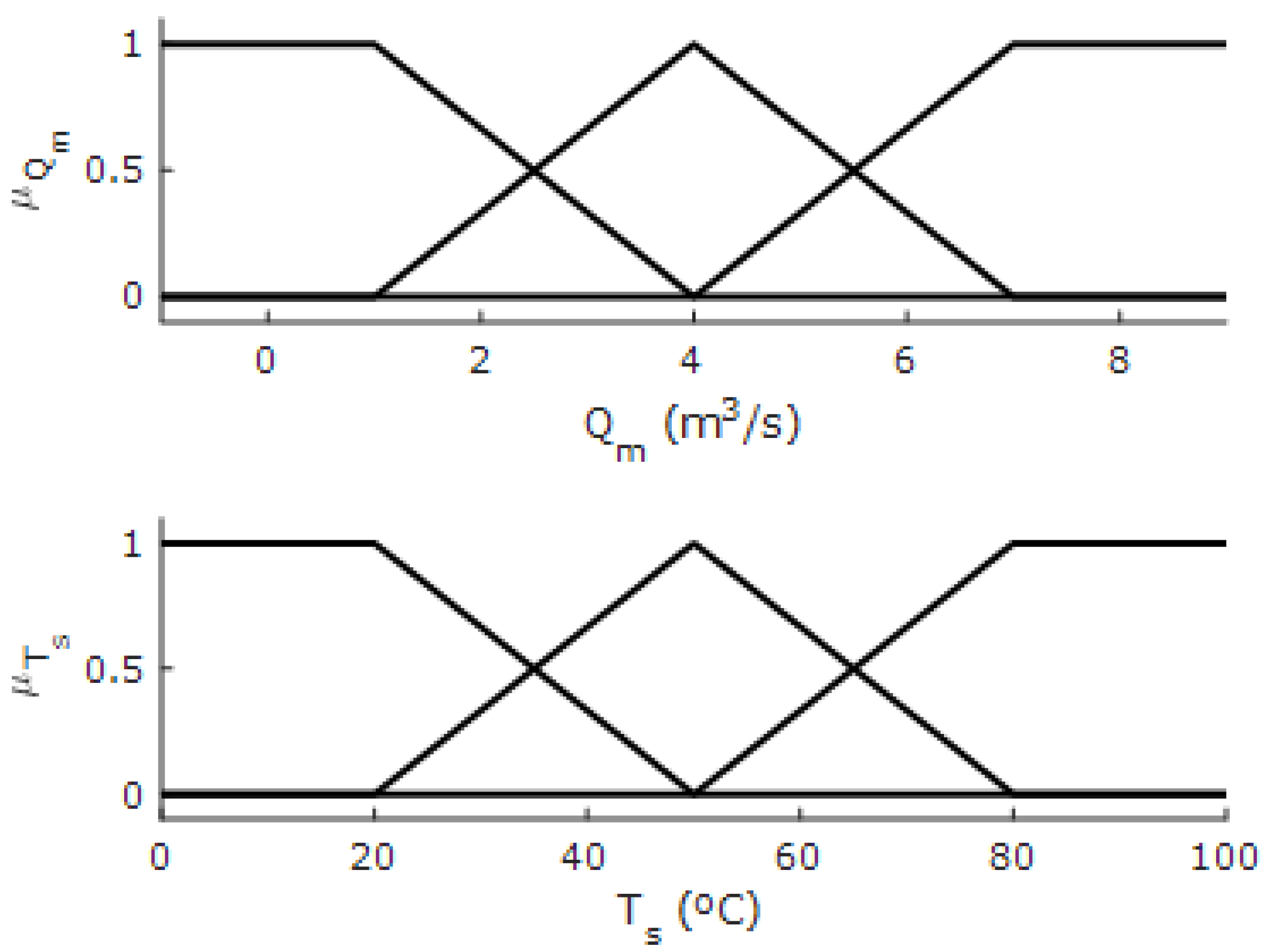
After generating the data as shown in the previous section, we next proceed to determine the membership functions in order to generate the fuzzy system, as shown in Figure 10.

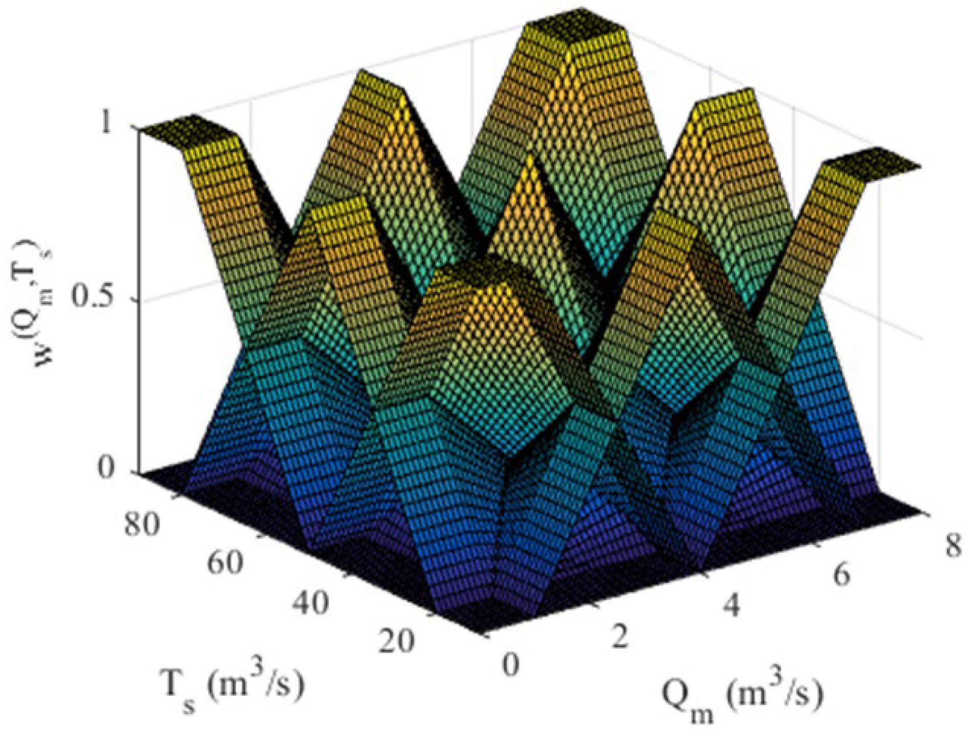
Through the fuzzy inference process, a total of nine rules are obtained, as shown in Figure 11.

Figure 12 shows the projections of the centers of the fuzzy rules obtained by the fuzzy inference process onto the workspace of the thermal mixing tank system. It can be seen that the top right [7.80] and bottom right [7.20] rules do not cover a significant working space and that samples requiring these fuzzy rules are rarely obtained. This is because working with flow rates requires the inlet valves to be opened, which causes the liquids to mix and the outlet temperature to be close to the average of the inlet temperatures.

The mean square error method is used here to comparison of the effectiveness of the different methodologies.

To identify the nonlinear system, the generalized T-S identification method is used. A least-squares identification of the linearized system at the nominal working point is performed using the ${\gamma }^2$ = 10 ⁻⁶ parameter. As a result, the following identification errors are obtained:

$$RMSE\left(er{r}_Q\right)=0.0026,RMSE\left(er{r}_T\right)=0.1128.$$

(69)

Based on the parameters identified for the nonlinear system, the incremental state model is obtained for each fuzzy rule [35]. Next, the incremental state model obtained for the central rule is provided as follows:

$$\begin{array}{cc}\hfill S^{(2,2)}: \mathrm{If} Q_m\left(k\right)& \mathrm{is} M_{Q_m}^2 \mathrm{and} T_S\left(k\right) \mathrm{is} M_{T_S}^2 \mathrm{then}:\hfill \\ \hfill x_a\left(k+1\right)& =A_a^{(2,2)}{x}_a\left(k\right)+B_a^{(2,2)}\delta \mathrm{u}\left(k\right)\hfill \\ \hfill y\left(k\right)& =C_a^{(2,2)}{x}_a\left(k\right),\hfill \end{array}$$

(70)

where

$$A_a^{(2,2)}=\left[\begin{array}{cccccccccccc}1& 0& 1.87& 1& 0& 0& 0& 0& 0& 0& 0& 0\\ 0& 1& 0& 0& 0& 0& 0& 0& 2.40& 1& 0& 0\\ 0& 0& 1.87& 1& 0& 0& 0& 0& 0& 0& 0& 0\\ 0& 0& -0.88& 0& 1& 0& 0& 0& 0& 0& 0& 0\\ 0& 0& 0& 0& 0& 1& 0& 0& 0& 0& 0& 0\\ 0& 0& 0& 0& 0& 0& 1& 0& 0& 0& 0& 0\\ 0& 0& 0& 0& 0& 0& 0& 1& 0& 0& 0& 0\\ 0& 0& 0& 0& 0& 0& 0& 0& 0& 0& 0& 0\\ 0& 0& 0& 0& 0& 0& 0& 0& 2.40& 1& 0& 0\\ 0& 0& 0& 0& 0& 0& 0& 0& -1.94& 0& 1& 0\\ 0& 0& 0& 0& 0& 0& 0& 0& 0.2& 0& 0& 1\\ 0& 0& 0& 0& 0& 0& 0& 0& 0& 0& 0& 0\end{array}\right],B_a^{(2,2)}=\left[\begin{array}{cc}0& 0\\ 0& 0\\ 0& 0\\ 0& 0\\ 0& 0\\ 0& 0.0061\\ 0.0052& -0.0013\\ 0.0002& 0\\ 0& 0\\ 0& -0.1696\\ 0.1236& 0.1030\\ -0.0616& 0\end{array}\right]$$

(71)

$$C_a^{(2,2)}=\left[\begin{array}{cccccccccccc}1& 0& 0& 0& 0& 0& 0& 0& 0& 0& 0& 0\\ 0& 1& 0& 0& 0& 0& 0& 0& 0& 0& 0& 0\end{array}\right].$$

(72)

For each fuzzy rule, the state feedback matrix is calculated using the discrete LQR method. The Q and R matrices used in the design are detailed below:

$$Q=0.1diag\left(\right[30.021111111111\left]\right);R=diag\left(\right[11\left]\right).$$

(73)

The feedback matrix $K^{(2,2)}$ obtained in the central rule is as follows:

$$\begin{array}{cc}& S^{(2,2)}: \mathrm{If} Q_m\left(k\right) \mathrm{is} M_{Q_m}^2 \mathrm{and} T_S\left(k\right) \mathrm{is} M_{T_S}^2 \mathrm{then}:\hfill \\ \hfill K^{(2,2)}=& \left[\begin{array}{cccccccccccc}0.1& 0.0& 14.0& 13.6& 13.1& 12.5& 11.9& 11.4& 1.2& 1.1& 1.1& 1.0\\ 0.1& -0.0& 11.9& 11.5& 11.0& 10.5& 10.0& 9.4& -1.2& -1.1& -1.0& -0.9\end{array}\right]\hfill \end{array}$$

(74)

The state observer in each fuzzy rule is obtained by means of the optimal state observer. The matrix $H^{(2,2)}$ obtained in the central rule is

$$\begin{array}{cc}\hfill S^{(2,2)}: \mathrm{If} Q_m\left(k\right)& \mathrm{is} M_{Q_m}^2 \mathrm{and} T_S\left(k\right) \mathrm{is} M_{T_S}^2 \mathrm{then}:\hfill \\ \hfill H^{(2,2)}& =\left[\begin{array}{cc}1.8770& 0\\ -0.8821& 0\\ 0& 0\\ 0& 0\\ 0& 0\\ 0& 0\\ 0& 0\\ 0& 0\\ 0& 2.4055\\ 0& -1.9350\\ 0& 0.5237\\ 0& 0\end{array}\right].\hfill \end{array}$$

(75)

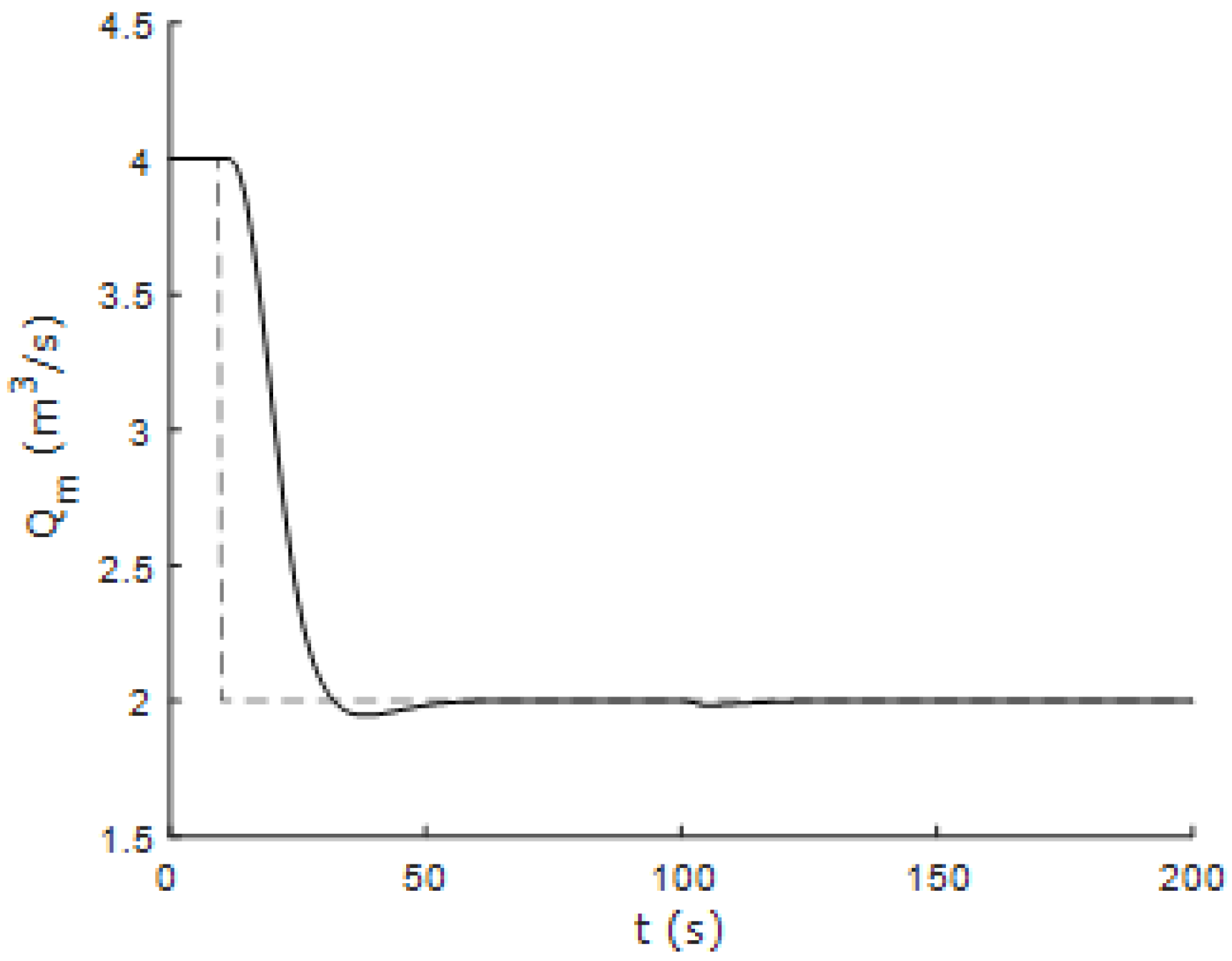
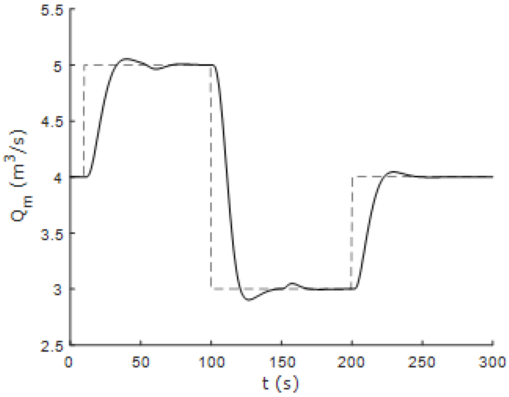
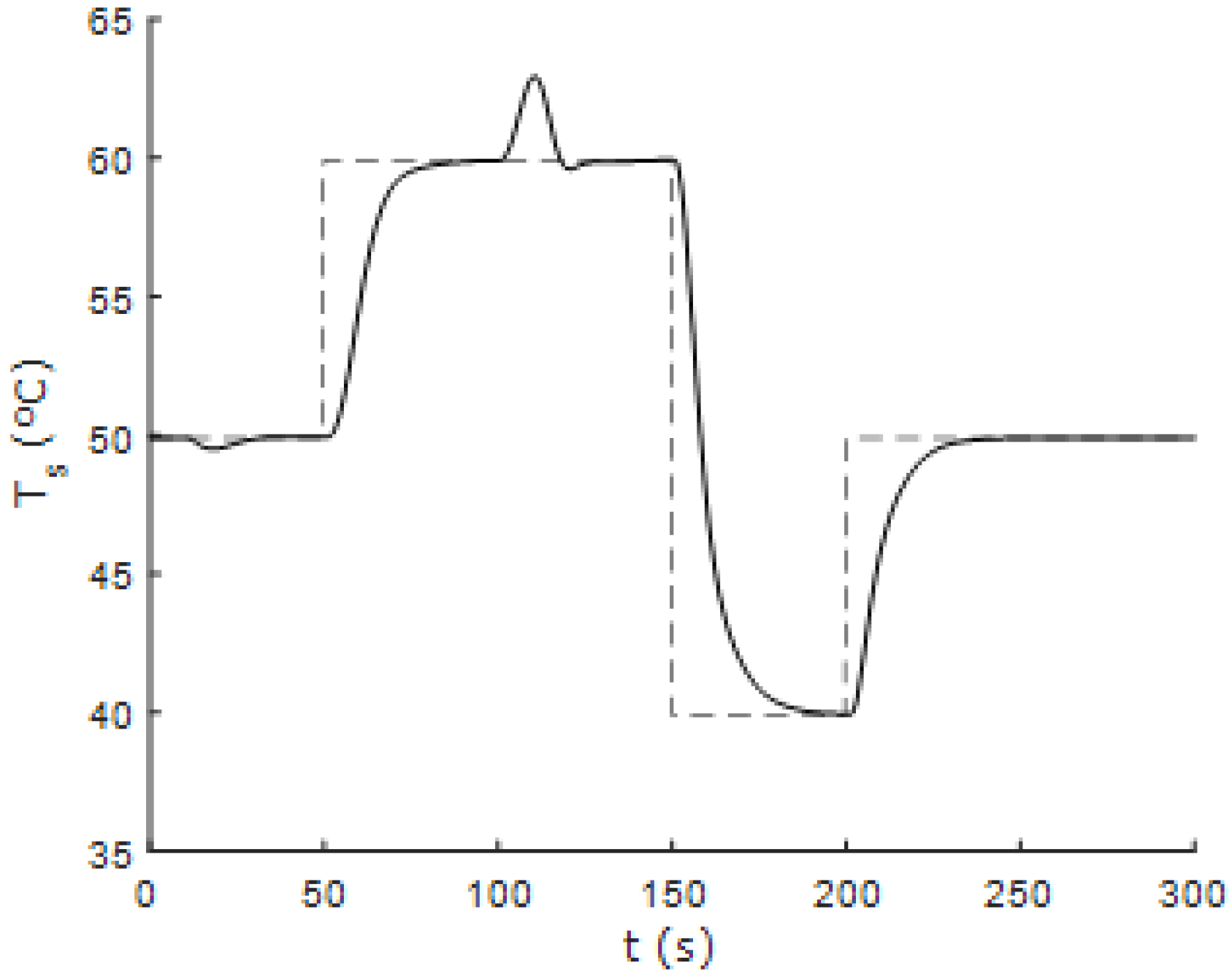
Figure 13 and Figure 14 show the response of the controlled system using the 1DMF method based on the fuzzy incremental state model using one-dimensional membership functions when the system is subjected to changes in the reference values of flow and temperature. Furthermore, Figure 15 and Figure 16 show the response of the controlled system to successive changes in the reference signals. It can be seen that the fuzzy controller performs correctly in areas away from the nominal operating point.

The traditional method based on one-dimensional membership functions is a suitable methodology for nonlinear control of the thermal mixing tank system. However, this method includes rules that have no relevance to the identification or control of this system. In order to reduce this set of unnecessary rules, methods based on MDMFs are proposed below.

4.2. Fuzzy Modeling and Fuzzy Control Based on MDMFs Fitted by the FCM Algorithm

This section describes modeling, identification, and fuzzy T-S control based on MDMFs tuned by means of the FCM algorithm and applied to the same example of a thermal mixing tank system.

In order to test whether there is any improvement in the nine rules specified by the traditional method in Section 4.1, we selected seven fuzzy rules defined by MDMFs. Becasue the design objective for the MDMFs is that they should cover the full working range of the thermal mixing tank system, the uniform data discussed above are used for the FCM algorithm. It should be noted that the data have been normalized to avoid the weight of the temperature in the distances being much larger than the weight of the flow rate due to the numerical difference between these two ranges.

The performance of this algorithm was tested with different values of the m parameter, which indicates the degree of overlap between the membership functions. As this parameter is increased, the slopes of the functions become smoother, which is not desirable.

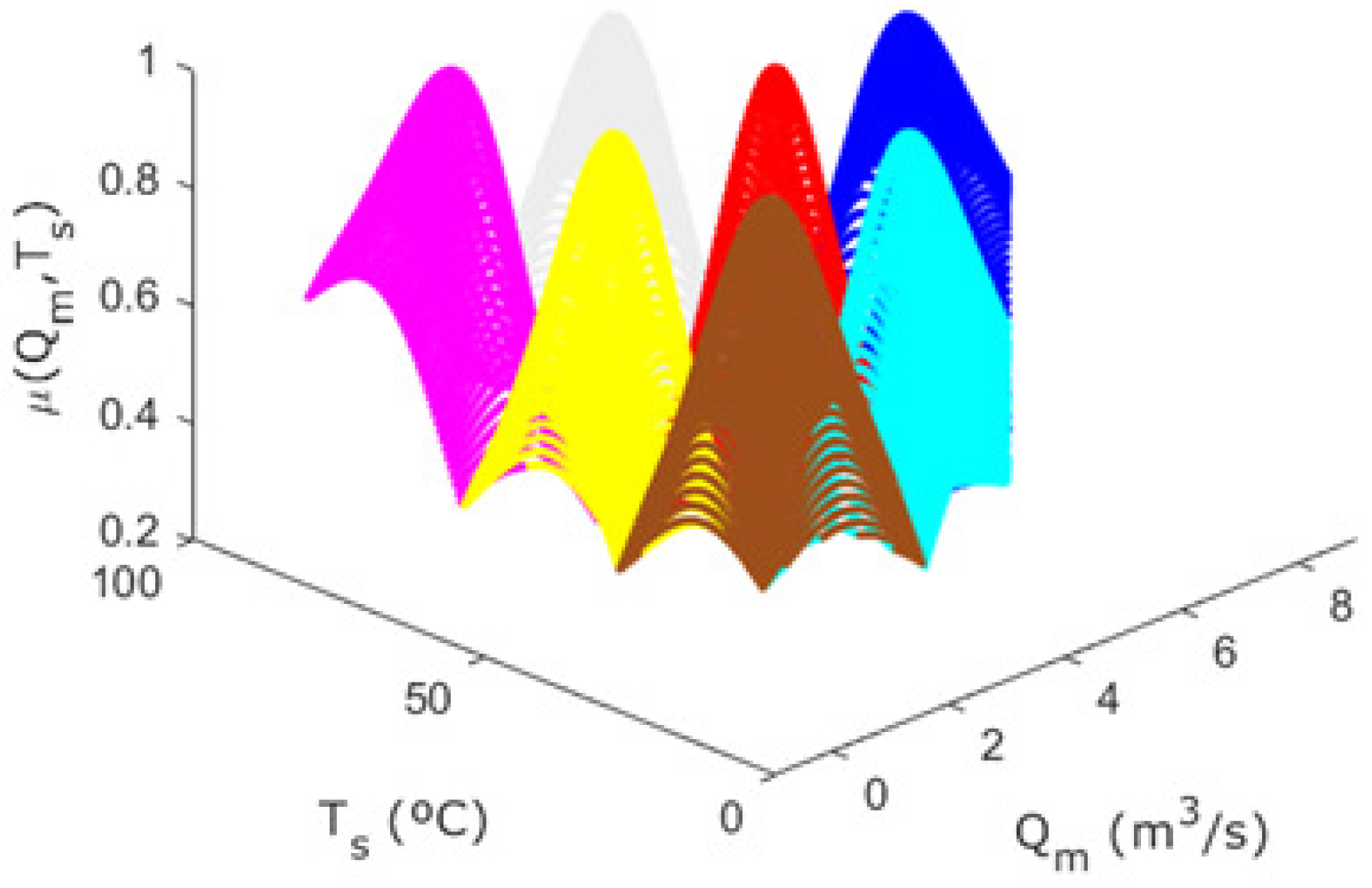
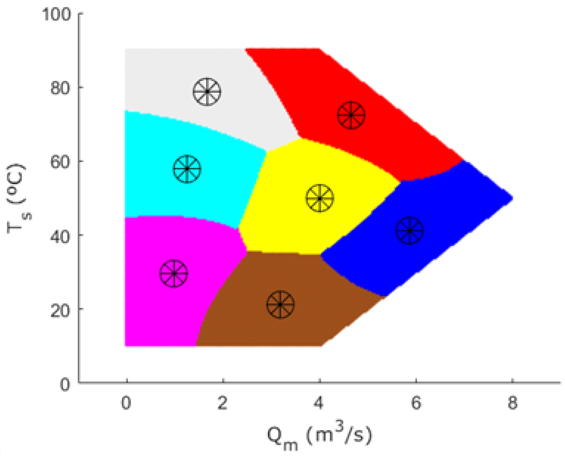
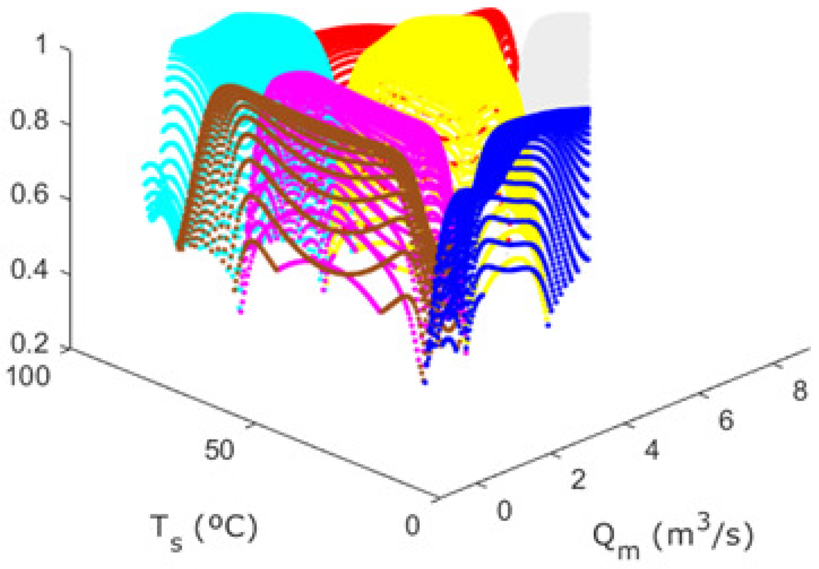
After several trials, a value of $m=2$ was selected, resulting in the MDMFs shown in Figure 17 at the conclusion of the FCM algorithm. The results of the FCM algorithm produce normalized centers that do not correspond to the workspace of the system under study. Therefore, both of the MDMFs must be denormalized in order to be represented on the workspace of the system.

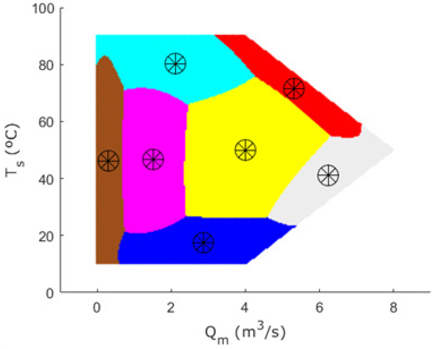
Figure 18 shows the areas of the workspace that are best represented by the different clusters obtained by the FCM algorithm. The centers of the clusters are also shown in the locations determined by the algorithm.

One of the cluster centers was intentionally located at point (4, 50), as this is the nominal operating point of the thermal mixing tank system.

When performing traditional identification by means of the membership functions fitted with the FCM algorithm, the following identification errors are obtained based on the open-loop data of the thermal mixing tank system:

$$RMSE\left(er{r}_Q\right)=0.0025, RMSE\left(er{r}_T\right)=0.0984.$$

(76)

It can be seen that these errors are smaller than those obtained in the previous section. Moreover, this accuracy level was reached with two fewer rules than required when using one-dimensional membership functions, allowing us to affirm an improvement in the modeling and identification of the system. However, having to normalize and then denormalize the samples in order to use this method is a problem that needs to be taken into account.

The following fuzzy vector variable z(k) is defined for all methodologies based on MDMFs:

$$z\left(k\right)=\left[\begin{array}{c}{Q}_m\left(k\right)\\ T_S\left(k\right)\end{array}\right].$$

(77)

As in the previous section, the incremental state model obtained for the central rule is

$$\begin{array}{cc}\hfill & S^{\left(1\right)}: \mathrm{If} z\left(k\right) \mathrm{is} M^{\left(1\right)} \mathrm{then}:\\ & x_a\left(k+1\right)=A_a^{\left(1\right)}{x}_a\left(k\right)+B_a^{\left(1\right)}\delta \mathrm{u}\left(k\right)\\ & y\left(k\right)=C_a^{\left(1\right)}{x}_a\left(k\right),\end{array}$$

(78)

where

$$A_a^{\left(1\right)}=\left[\begin{array}{cccccccccccc}1& 0& 1.83& 1& 0& 0& 0& 0& 0& 0& 0& 0\\ 0& 1& 0& 0& 0& 0& 0& 0& 2.26& 1& 0& 0\\ 0& 0& 1.83& 1& 0& 0& 0& 0& 0& 0& 0& 0\\ 0& 0& -0.84& 0& 1& 0& 0& 0& 0& 0& 0& 0\\ 0& 0& 0& 0& 0& 1& 0& 0& 0& 0& 0& 0\\ 0& 0& 0& 0& 0& 0& 1& 0& 0& 0& 0& 0\\ 0& 0& 0& 0& 0& 0& 0& 1& 0& 0& 0& 0\\ 0& 0& 0& 0& 0& 0& 0& 0& 0& 0& 0& 0\\ 0& 0& 0& 0& 0& 0& 0& 0& 2.26& 1& 0& 0\\ 0& 0& 0& 0& 0& 0& 0& 0& -1.72& 0& 1& 0\\ 0& 0& 0& 0& 0& 0& 0& 0& 0.44& 0& 0& 1\\ 0& 0& 0& 0& 0& 0& 0& 0& 0& 0& 0& 0\end{array}\right],B_a^{\left(1\right)}=\left[\begin{array}{cc}0& 0\\ 0& 0\\ 0& 0\\ 0& 0\\ 0& 0\\ 0& 0.0090\\ 0.0083& -0.0004\\ -0.0008& 0\\ 0& 0\\ 0& -0.3351\\ 0.2935& 0.1572\\ -0.1360& 0\end{array}\right].$$

(79)

The C matrix is the same as in the 1DMFs. The state feedback matrix is calculated using the same algorithm as in Section 4.1. The Q and R matrices used in the design are the same as in the previous algorithm. The feedback matrix ${\mathsf{K}}^{\left(1\right)}$ obtained in the central rule is

$$\begin{array}{cc}\hfill & S^{\left(1\right)}: \mathrm{If} z\left(k\right) \mathrm{is} M^{\left(1\right)}\mathrm{then}:\hfill \\ \hfill K^{\left(1\right)}=& \left[\begin{array}{cccccccccccc}0.1& 0.0& 8.7& 8.5& 8.18& 7.8& 7.5& 7.0& 0.6& 0.6& 0.6& 0.5\\ 0.1& -0.0& 7.0& 6.8& 6.5& 6.2& 5.8& 5.5& -0.7& -0.7& -0.6& -0.5\end{array}\right].\hfill \end{array}$$

(80)

The state observer in each fuzzy rule is again obtained using the optimal state observer method, as in Section 4.1. The matrix $H^{\left(1\right)}$ obtained in the central rule is

$$S^{\left(1\right)}: \mathrm{If} z\left(k\right) \mathrm{is} M^{\left(1\right)} \mathrm{then}:$$

$$H^{\left(1\right)}=\left[\begin{array}{cc}1.8287& 0\\ -0.8387& 0\\ 0& 0\\ 0& 0\\ 0& 0\\ 0& 0\\ 0& 0\\ 0& 0\\ 0& 2.2597\\ 0& -1.7158\\ 0& 0.4428\\ 0& 0\end{array}\right].$$

(81)

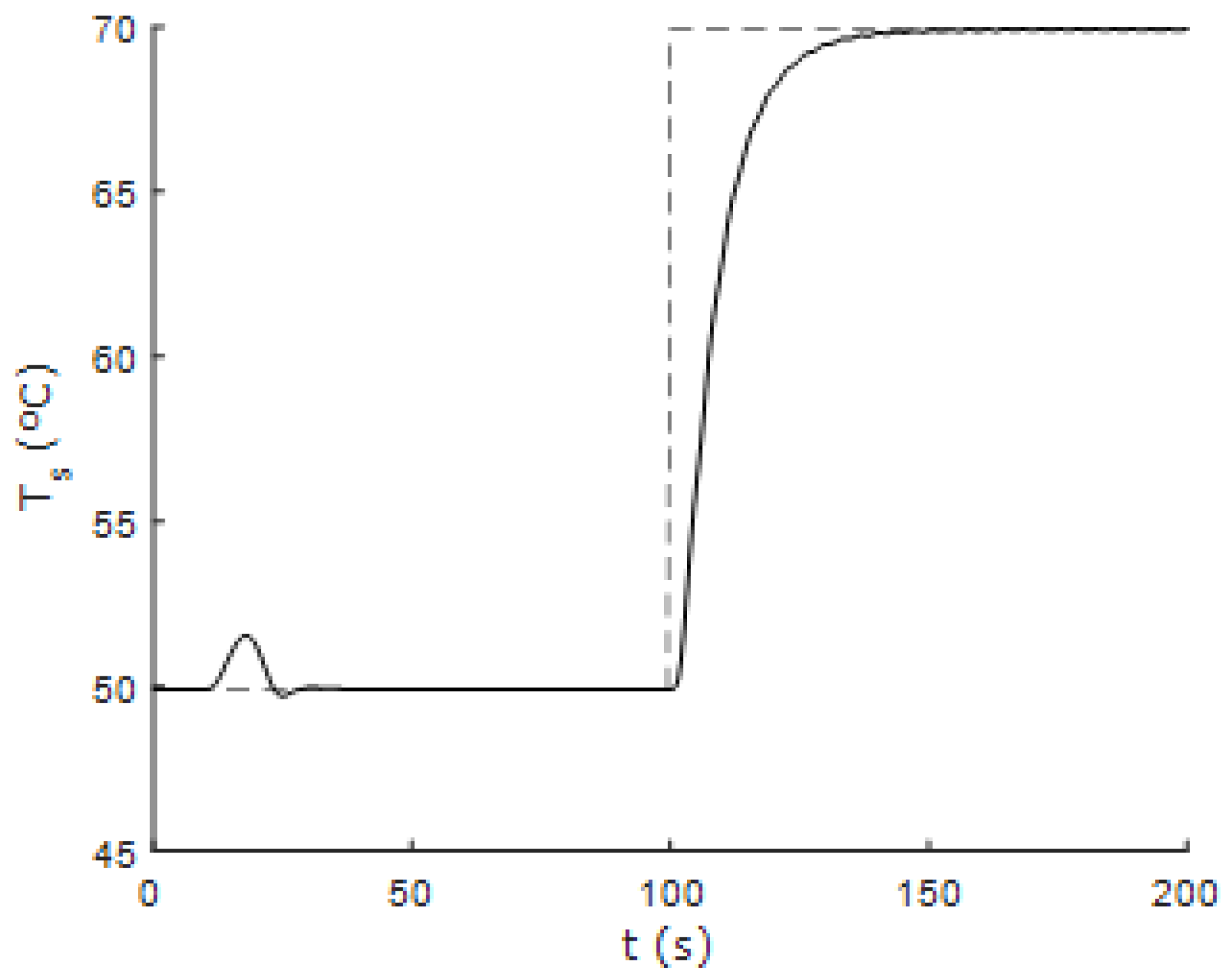
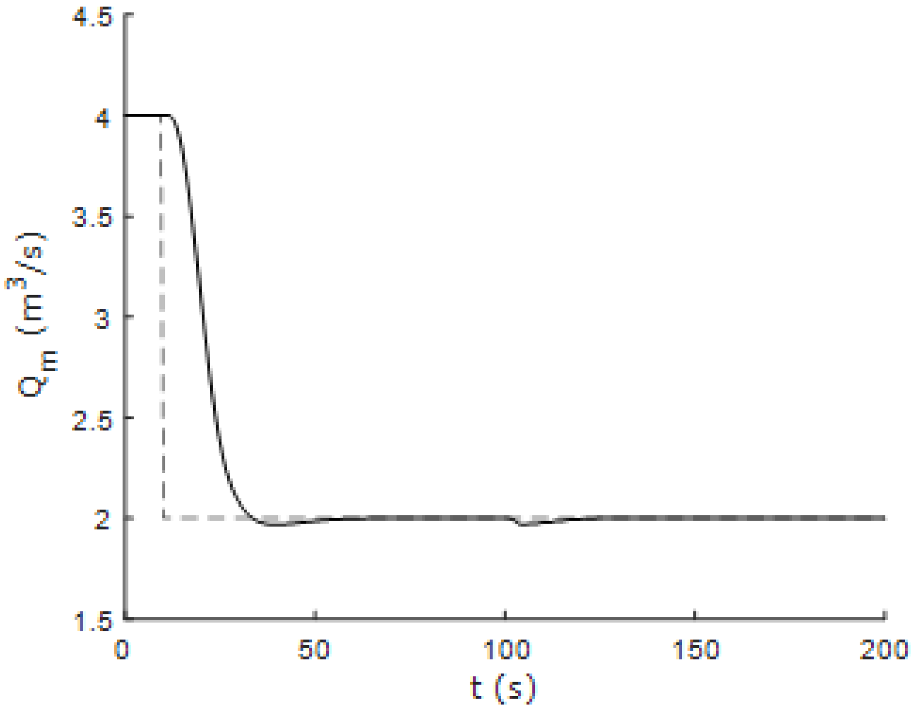
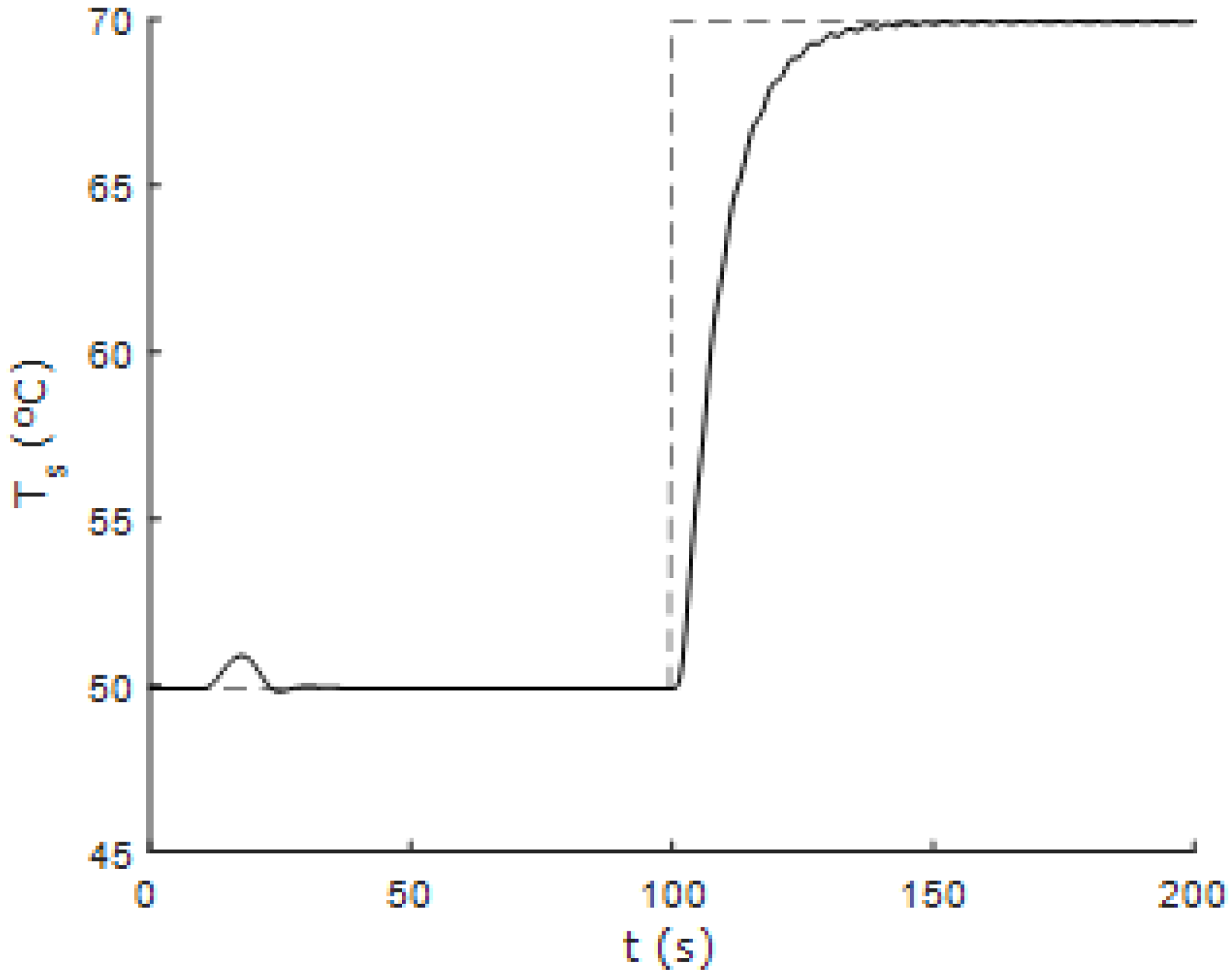
Figure 19 and Figure 20 show the response of the system based on the fuzzy incremental state model using MDMFs defined by the FCM method when the system is subjected to changes in the reference values of flow and temperature. Furthermore, Figure 21 and Figure 22 show the response of the controlled system to successive changes in the reference signals. It can be seen that the fuzzy controller performs correctly in areas far from the nominal operating point.

This method also achieves efficient control of the thermal mixing tank system by using fewer fuzzy rules. On the other hand, the process of normalizing and denormalizing the data in order to use the FCM algorithm can be very prone to error, and special care needs to be taken in this respect.

4.3. Fuzzy Modeling and Control Based on MDMFs Fitted by the GK Algorithm

In this section, we establish modeling, identification, and fuzzy T-S control based on MDMFs adjusted by means of the GK algorithm.

Seven clusters are chosen in order to check whether there is any improvement over the seven rules specified in the FCM algorithm. Uniform samples are used in order to avoid modifications in the position of the cluster centers due to the massive clustering of data in certain parts of the working area. It should be noted that the samples do not need to be normalized, which represents an immediate advantage over the FCM algorithm. The $m=2$ parameter is used in the same way as previously.

Figure 23 shows the shapes of the MDMFs obtained after applying the GK algorithm. Figure 24 shows the set of samples of the system and their membership in the most representative cluster. The centers of the clusters are shown in the locations determined by the algorithm.

One of the cluster centers was deliberately located at the point (4, 50), as this is the nominal working point of the system.

When using traditional identification by means of membership functions adjusted with the GK algorithm, the following identification errors are obtained based on the open-loop data of the thermal mixing tank system:

$$RMSE\left(er{r}_Q\right)=0.0025,RMSE\left(er{r}_T\right)=0.0865.$$

(82)

It can be observed that the ratios of these errors are lower than those obtained using the FCM algorithm. Furthermore, it is not necessary to normalize and denormalize the samples and cluster centers, allowing us to affirm that this system represents a great advantage with respect to the FCM algorithm.

Recalling the incremental state model obtained in (78), the matrices are

$$A_a^{\left(1\right)}=\left[\begin{array}{cccccccccccc}1& 0& 1.87& 1& 0& 0& 0& 0& 0& 0& 0& 0\\ 0& 1& 0& 0& 0& 0& 0& 0& 2.43& 1& 0& 0\\ 0& 0& 1.87& 1& 0& 0& 0& 0& 0& 0& 0& 0\\ 0& 0& -0.88& 0& 1& 0& 0& 0& 0& 0& 0& 0\\ 0& 0& 0& 0& 0& 1& 0& 0& 0& 0& 0& 0\\ 0& 0& 0& 0& 0& 0& 1& 0& 0& 0& 0& 0\\ 0& 0& 0& 0& 0& 0& 0& 1& 0& 0& 0& 0\\ 0& 0& 0& 0& 0& 0& 0& 0& 0& 0& 0& 0\\ 0& 0& 0& 0& 0& 0& 0& 0& 2.43& 1& 0& 0\\ 0& 0& 0& 0& 0& 0& 0& 0& -1.92& 0& 1& 0\\ 0& 0& 0& 0& 0& 0& 0& 0& 0.49& 0& 0& 1\\ 0& 0& 0& 0& 0& 0& 0& 0& 0& 0& 0& 0\end{array}\right],B_a^{\left(1\right)}=\left[\begin{array}{cc}0& 0\\ 0& 0\\ 0& 0\\ 0& 0\\ 0& 0\\ 0& 0.0103\\ 0.0085& -0.0015\\ -0.0020& 0\\ 0& 0\\ 0& -0.4749\\ 0.2062& 0.2333\\ -0.1061& 0\end{array}\right]$$

(83)

and the C matrix is the same as in the previous methods. The Q and R matrices used in the design are also the same ones used before. The feedback matrix ${\mathsf{K}}^{\left(1\right)}$ obtained in the central rule is

$$\begin{array}{cc}& S^{\left(1\right)}: \mathrm{If} z\left(k\right) \mathrm{is} M^{\left(1\right)} \mathrm{then}:\hfill \\ \hfill K^{\left(1\right)}=& \left[\begin{array}{cccccccccccc}0.1& 0.0& 7.5& 7.2& 6.8& 6.4& 6.1& 5.7& 3.0& 2.8& 2.6& 2.5\\ 0.1& -0.0& 18.3& 17.8& 17.1& 16.4& 15.7& 15.1& -1.8& -1.7& -1.6& -1.6\end{array}\right]\hfill \end{array}$$

(84)

The state observer in each fuzzy rule is again obtained by means of the optimal state observer. The matrix obtained in the central rule is

$$\begin{array}{c}\hfill S^{\left(1\right)}: \mathrm{If} z\left(k\right) \mathrm{is} M^{\left(1\right)} \mathrm{then}:\\ \hfill H^{\left(1\right)}=\left[\begin{array}{cc}1.8603& 0\\ -0.8681& 0\\ 0& 0\\ 0& 0\\ 0& 0\\ 0& 0\\ 0& 0\\ 0& 0\\ 0& 2.3085\\ 0& -1.8628\\ 0& 0.5403\\ 0& 0\end{array}\right]\end{array}$$

(85)

Figure 25 and Figure 26 show the response of the system controlled using MDMFs defined by the GK method when the system is subjected to changes in the reference values of flow and temperature. Furthermore, Figure 27 and Figure 28 show the response of the controlled system to successive changes in the reference signals. It can be seen that the fuzzy controller performs correctly in areas away from the nominal operating point.

This method is valid for identification and control; in addition, it has has fewer rules than the traditional method. It can be observed that the errors are smaller than those obtained for the methods in the previous section. Moreover, it is not necessary to normalize and denormalize the samples in order to apply this algorithm, making it the best solution among the studied methods for fuzzy control based on MDMFs.

4.4. Fuzzy Modeling and Control Based on MDMFs Fitted by the GG Algorithm

This section establishes the modeling, identification, and fuzzy control of T-S based on MDMFs fitted by means of the GG algorithm.

To check whether there is any improvement over the seven rules specified in the previous section, we again used seven clusters. Uniform samples were used in order to avoid changes in the position of the cluster centers due to the massive clustering of data in certain parts of the working area.

Figure 29 shows the shapes of the MDMFs obtained after applying the GG algorithm. Figure 30 shows the set of samples of the system and their membership in the cluster that best represents them. The centers of the clusters are also depicted in order to show where the algorithm determined that they should be located.

We deliberately located one of the cluster centers at the point (4, 50), as this is the nominal working point of the system.

When performing T-S identification by means of the membership functions fitted with the GG algorithm, the following identification errors were obtained based on the open-loop data of the thermal mixing tank system:

$$RMSE\left(er{r}_Q\right)=0.0026,RMSE\left(er{r}_T\right)=0.1061.$$

Recalling the incremental state model obtained in (78), the matrices are

$$A_a^{\left(1\right)}=\left[\begin{array}{cccccccccccc}1& 0& 1.79& 1& 0& 0& 0& 0& 0& 0& 0& 0\\ 0& 1& 0& 0& 0& 0& 0& 0& 2.03& 1& 0& 0\\ 0& 0& 1.79& 1& 0& 0& 0& 0& 0& 0& 0& 0\\ 0& 0& -0.81& 0& 1& 0& 0& 0& 0& 0& 0& 0\\ 0& 0& 0& 0& 0& 1& 0& 0& 0& 0& 0& 0\\ 0& 0& 0& 0& 0& 0& 1& 0& 0& 0& 0& 0\\ 0& 0& 0& 0& 0& 0& 0& 1& 0& 0& 0& 0\\ 0& 0& 0& 0& 0& 0& 0& 0& 0& 0& 0& 0\\ 0& 0& 0& 0& 0& 0& 0& 0& 2.02& 1& 0& 0\\ 0& 0& 0& 0& 0& 0& 0& 0& -1.46& 0& 1& 0\\ 0& 0& 0& 0& 0& 0& 0& 0& 0.41& 0& 0& 1\\ 0& 0& 0& 0& 0& 0& 0& 0& 0& 0& 0& 0\end{array}\right],B_a^{\left(1\right)}=\left[\begin{array}{cc}0& 0\\ 0& 0\\ 0& 0\\ 0& 0\\ 0& 0\\ 0& 0.0103\\ 0.0159& -0.0005\\ -0.0049& 0\\ 0& 0\\ 0& -1.0111\\ 0.8258& 0.3329\\ -0.4853& 0\end{array}\right].$$

(86)

The C matrix is the same as in previous methods, and the Q and R matrices are also the same. The feedback matrix ${\mathsf{K}}^{\left(1\right)}$ obtained in the central rule is

$$S^{\left(1\right)}: \mathrm{If} z\left(k\right) \mathrm{is} M^{\left(1\right)} \mathrm{then}:$$

$$K^{\left(1\right)}=\left[\begin{array}{cccccccccccc}0.1& 0.0& 13.1& 12.7& 12.2& 11.6& 11.1& 10.5& 2.4& 2.2& 2.0& 1.9\\ 0.1& -0.0& 11.7& 11.3& 10.8& 10.3& 9.8& 9.2& -2.3& -2.1& -1.9& -1.7\end{array}\right].$$

(87)

The state observer in each fuzzy rule is again obtained by the optimal state observer method. The matrix ${\mathsf{H}}^{(2,2)}$ obtained in the central rule is

$$\begin{array}{c}\hfill S^{\left(1\right)}: \mathrm{If} z\left(k\right) \mathrm{is}{M}^{\left(1\right)}\mathrm{then}:\\ \hfill H^{\left(1\right)}=\left[\begin{array}{cc}1.8718& 0\\ -0.8771& 0\\ 0& 0\\ 0& 0\\ 0& 0\\ 0& 0\\ 0& 0\\ 0& 0\\ 0& 2.6091\\ 0& -2.2878\\ 0& 0.6758\\ 0& 0\end{array}\right].\end{array}$$

(88)

Figure 31 and Figure 32 show the response of the system controlled by the GG algorithm when the system is subject to changes in the reference values of the flow and temperature. Furthermore, Figure 33 and Figure 34 show the response of the controlled system to successive changes in the reference signals. It can be seen that the fuzzy controller acts correctly in areas far from the nominal operating point.

It should be noted that the samples do not need to be normalized, which represents an immediate advantage over the FCM algorithm. However, having to rely on a more robust algorithm to determine a non-random initial participation matrix means that the GG algorithm is at a disadvantage with respect to the GK algorithm.

It can be seen that the errors are greater than those obtained using the GK method. Moreover, from an intuitive point of view, the form of the clusters does not seem very suitable for generating MDMFs, which makes it the worst solution among those proposed in this work.

5. Comparison of Clustering Methods for Fuzzy System Modeling

The identification results obtained for the thermal mixing tank system using the four proposed methods (one-dimensional membership functions, FCM algorithm, GK algorithm, and GG algorithm are summarized below, with the root mean squared error (RMSE) calculated for each of the four methods. The obtained results are summarized in

Table 1. Errors in the identification of the nonlinear system.

Identification Type	$\mathbf{RMSE}\left({\mathbf{err}}_{\mathbf{Q}}\right)$	$\mathbf{RMSE}\left({\mathbf{err}}_{\mathbf{T}}\right)$	Mean of RMSE
One-dimensional membership functions	0.0026	0.1128	0.0577
FCM algorithm	0.0025	0.0984	0.0505
GK algorithm	0.0025	0.0865	0.0445
GG algorithm	0.0026	0.1061	0.0544

.

The FCM fuzzy clustering algorithm offers an improvement over results obtained using 1DMFs, achieving better control of the system with a reduced number of rules. On the other hand, the process of data normalization and denormalization required by the FCM algorithm can be very susceptible to errors, and special care must be taken in this aspect.

The GK fuzzy clustering algorithm has a lower identification error than the FCM algorithm with the same reduced number of rules; moreover, it is not necessary to normalize the data, which makes it the best option with respect to other methods.

Regarding the GG algorithm, the main drawback is that it requires an initial participation matrix, meaning that it requires previous execution of another fuzzy clustering algorithm. Furthermore, this algorithm presents a higher identification error than the GK algorithm. Finally, from an intuitive point of view, the shape of the obtained clusters does not seem very suitable for the generation of MDMFs. For these reasons, this algorithm is the worst solution of those proposed in this work for the modeling, identification, and fuzzy control of nonlinear systems.

6. Conclusions

In this work, we have developed a method for the modeling, identification, and control of nonlinear systems by means of the T-S model based on MDMFs. We considered the use of three different fuzzy clustering algorithms to adjust the MDMFs: FCM, GK, and GG.

The proposed methodology was validated through the identification and control of a thermal mixing tank system using both one-dimensional membership functions (1DMFs) and MDMFs. The results demonstrate that 1DMFs do not provide an optimal control solution, as they generate fuzzy rules that occur at points far from the working area.

The main contribution of this paper is to demonstrate that MDMFs fitted using clustering techniques such as the FCM, GK, and GG algorithms can achieve lower identification errors compared to traditional fuzzy inference methods while requiring fewer fuzzy rules. This finding has important implications for applications in control engineering contexts where the efficiency and accuracy of system modeling is crucial.