Abstract
This paper aims to study a two-degree-of-freedom (2DOF) magnetic spring-based electromagnetic generator system theoretically and experimentally. The proposed linear generator system contains a nonlinear nonmagnetic shaft (nonmagnetic materials), two floating magnets, and two fixed magnets. All magnets are placed in the system in a repulsive configuration. First, the magnetic properties of the proposed system are studied to provide insight into its role in the system’s nonlinear oscillatory behavior. The magnetic restoring forces are analyzed, and both linear and nonlinear coefficients of the oscillator system are analyzed based on these forces. The mathematical model of the proposed system is presented to study the dynamic behaviors of the oscillator system. The magnetic restoring forces and dynamic behaviors for different oscillator heights are also studied. Finally, the proposed system’s energy generation capacity is examined using electromechanical coupling.
1. Introduction
In light of the pressing energy crisis exacerbated by the challenges of the pandemic, the need to explore alternative energy sources has become more urgent than ever. One promising avenue that has gained significant attention involves harvesting energy from vibrating environments [1,2,3,4,5]. This surge in diverse vibration-energy-harvesting techniques has sparked a fervent pursuit for improved output performance and operational efficiency. In this context, electromagnetic-energy-harvesting systems utilizing magnetic levitation architectures offer unique advantages [6,7,8,9,10]. These include more superficial mechanical structures, higher output power, and reduced costs, making them particularly well suited for track and vehicle monitoring applications.
Initial investigations predominantly concentrated on linear dynamic energy harvesters, which, unfortunately, were limited to operating within narrow bandwidths and struggled to amplify output power under low-energy excitation [11]. However, nonlinear energy harvesters have effectively mitigated these constraints, addressing the narrow working bandwidth issue inherent in their linear counterparts and ensuring robust output performance near the designated working frequency. Using real data, linear and nonlinear oscillator systems have been compared, and it has been demonstrated that nonlinear oscillators have the highest power output in most cases. Still, nonlinear oscillators have a wider frequency bandwidth for harvesting energy [12]. Owens et al. found that nonlinear oscillating systems are better than linear oscillators for extending the frequency response bandwidth [13]. Researchers have proposed and developed nonlinear oscillator (magnetic levitation)-based electromagnet energy harvesters to harness energy from vibrations such as handshaking, human motion, and the environment. Saravia et al. showed that a magnetic levitation-based electromagnetic generator could be an interesting alternative to generate energy from vibration sources, especially low-frequency sources [14]. The magnetic spring-based system has a straightforward construction structure and low maintenance costs. The magnetic spring system has been used in translator design to make the oscillator nonlinear, which is more effective in the broadband frequency range, especially in low-frequency ocean environments [15]. In a single-degree-of-freedom (SDOF) magnetic spring-based system, the magnetic spring works like a physical spring and is created when two magnets face each other in the same poles (North–North or South–South). When two magnets are placed with like poles facing each other (either N-N or S-S), they experience a repulsive force. If they are closer together, the repulsion becomes stronger and stronger, meaning the force increases nonlinearly with decreasing distance. This behavior mimics a mechanical spring, but unlike a linear spring (where force increases linearly with displacement), this magnetic repulsion increases nonlinearly.
SDOF magnetic spring-based oscillator systems have been used in electromagnetic energy harvesters to harvest energy [16]. Pedro Carneiro et al. presented a detailed review of the architectures of a single-degree-of-freedom (SDOF)-based magnetic levitation system-based electromagnetic energy generator [17]. The geometric and constructive parameters, optimization approaches, and energy-generating performances of twenty-one design configurations were compared. This review also looked at the most significant advanced models (finite element method, empirical, analytical, and semi-analytical) that were utilized to explain the physical phenomena of their transduction mechanisms. The SDOF magnetic spring-based system has only one degree of freedom and is limited to only one resonant frequency. The energy generator should pick up and resonate at every frequency present in the vibration source. One can use two resonant frequencies and achieve maximum power by employing a two-degrees-of-freedom (2DOF) oscillator system. The simplest form of a 2DOF system has two floating magnets and two fixed magnets. Kangqi Fan et al. proposed a two-degrees-of-freedom (2DOF) electromagnetic energy harvester (EMEH) using a magnetically levitating 1DOF oscillator system in a cylindrical housing to harvest energy from human body motion [18]. The theoretical model of the 2DOF EMEH was validated experimentally. The experimental results showed that the performance of the 2DOF system is much better than that of the 1DOF system-based energy harvester. However, the magnetic restoring, linear and nonlinear coefficient, and system dynamics were not studied. Moreover, 2DOF magnetic spring-based electromagnetic energy harvesters have been studied numerically and experimentally [19]. The proposed model consisted of two floating magnets and a bottom fixed magnet. The model did not have any top fixed magnet; therefore, the top floating magnet can oscillate with low frequencies. The proposed system has two resonance frequencies tuned to two fundamental frequencies. The proposed model was studied numerically and experimentally for vehicle monitoring, particularly railway monitoring applications. The findings showed that the 2DOF system improved performance by 10% compared with the 1DOF configuration.
From the literature, it has been seen that some research works have been conducted based on 2DOF magnetic spring-based electromagnetic generator systems [18,19,20]. However, no single paper in the literature has validated the theoretical model with the experimental model of the 2DOF magnetic-based electromagnetic generator systems. The dynamics of the proposed linear generator system are very important for deeply understanding and developing electromagnetic generator systems. Therefore, this paper aims to investigate the dynamics of a 2DOF magnetic spring-based generator system analytically and experimentally and the power generation capabilities of the electromagnetic generator system. This paper deals with the architecture of the 2DOF magnetic spring-based linear generator system, analytical modelling, the system’s behavior in relation to various design criteria, and an experimental analysis of the proposed linear generator system.
2. Architecture of the Two-Degrees-of-Freedom (2DOF) Electromagnetic Generator/Energy Harvester
The basic architecture of the electromagnetic generator or energy harvester contains four-ring permanent magnets (axially magnetized), a circular shaft, and winding coils. The 2DOF energy harvester is designed so that every function’s performance (such as magnetic restoring forces and induced voltage) should not affect or influence each magnet’s magnetic field, particularly when the floating magnets move. Minimizing the harmful cogging force (caused by the magnetic attraction between the stator and the permanent magnets mounted on the translator, leading to undesirable vibrations, noise, and a ripple in the thrust force) generated from the magnets and coil movement is required. Different nonmagnetic materials were used to avoid magnetic field interference. The polarity of the magnets is arranged so that the levitating magnet experiences a repulsive force because of the fixed magnets. A few multilayer coils are attached around the outer surface of the two floating magnets. The height and diameter of the shaft are 550 mm and 12 mm, respectively. Figure 1 presents the test rig setup with winding coils.

Figure 1.
Test rig of the proposed 2DOF system.
Figure 2 presents the schematic of the 2DOF system. The magnetic poles are oriented (NS-SN-NS-SN) to repel each other. The height and width of the test rig are 550 mm and 300 mm, respectively. The equilibrium height of the 2DOF oscillator is 303 mm; therefore, the fourth magnet is attached and locked to the vertical shaft 303 mm away from the first magnet. Two winding coils were added to the test rig, and both are connected to the data acquisition system to capture the induced voltages. Winding coil 1 was placed outside the first floating magnet, whereas winding coil number 2 was placed outside the second floating magnet. In Figure 1, sensor 1 is positioned on top of the bottom fixed magnet to measure the displacement of the first floating magnet, and sensor 2 is positioned underneath the top fixed magnet to measure the displacement of the second floating magnet. Reflective sensors (GP2Y0A41SK0F, Sharp) were used to measure the displacement of the floating magnets. The GP2Y0A41SK0F is a distance-measuring sensor, consisting of a PSD (position-sensitive detector), an IR-LED (infrared-emitting diode), and a signal processing circuit. The sensor’s output signal is voltage, and the relationship between this sensor’s output voltage and the inverse of the calculated distance is nearly linear over the sensor’s usable range. The sensor’s output voltage is converted to an estimated distance by constructing a best-fit line that relates the inverse of the output voltage (V) to distance (mm).
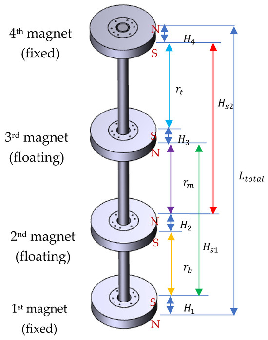
Figure 2.
Magnetic system where the two magnets are floating.
3. Magnetic Restoring Force of 2DOF-Based Energy Harvester
The magnetic poles of each magnet are oriented to repel the adjacent magnet, causing the floating magnets to be suspended by the nonlinear restoring force. The system’s nonlinear behavior allows the linear response to be modified by simply varying the position of the floating magnet between the top (fourth magnet) and bottom (first magnet) magnets. The magnetic force between the first magnet (fixed magnet) and second magnet (floating magnet) can be written as it was in [21,22],
where is the distance between the first and second magnet poles. and are the magnetic field intensities of the first and second magnets, respectively. The permeability of the air is . Similarly, Equation (1) can be rewritten for the second magnet (first floating magnet from the bottom magnet) and third magnet (second floating magnet) as
where is the distance between the second magnet and third magnet poles. Equation (1) can also be rewritten for the third magnet (second floating magnet) and fourth magnet (top fixed magnet) as
where is the distance between the third magnet and fourth magnet poles. For the case of in-plane movement, the expression for and can be written as
Moreover, for the case of in-plane movement, the expression for and can be written as
where is the distance between the upper surface of the bottom magnet and the lower surface of the third magnet. On the other hand, is between the upper surface of the second magnet and the lower surface of the fourth magnet. , , and are the heights of the first, second, third, and fourth magnets, respectively. To determine the magnetic restoring force for the first moving magnet, the second moving magnet is considered a fixed magnet. To measure the magnetic restoring force for the second moving magnet, the first moving magnet is considered a fixed magnet. The distance y2 represents the first moving magnet (second magnet), and the distance y3 represents the second moving magnet (third magnet); the resultant magnetic forces or magnetic spring restoring forces ( and ) applied to the moving magnets can be calculated as
The magnetic spring’s restoring forces can be calibrated from the calculation of the restoring force [23]. A Taylor series can express the Equations (6) and (7) as
where and are the linear constants. The nonlinear constants are denoted by , , , and . Figure 3 presents the analytical and numerical magnetic restoring forces for different positions of the first and second floating magnets.

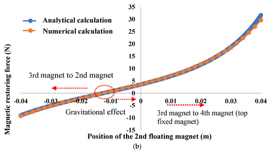
Figure 3.
Magnetic restoring force of (a) 1st floating magnet and (b) 2nd floating magnet.
The distance between the second magnet (first floating magnet) and first magnet (fixed magnet) is smaller than the distance between the second (first floating magnet) and third magnet (second floating magnet). Therefore, the magnetic restoring force is higher between the first and second magnets (second floating magnet) than the restoring force between the second and third magnets, as presented in Figure 3a. Similarly, the distance between the third magnet (second floating magnet) and second magnet (first floating magnet) is smaller than the distance between the third magnet and fourth magnet (fixed magnet). As a result, the magnetic restoring force between the third and second magnets is higher than the magnetic restoring force between the third and fourth magnets, as seen in Figure 3b.
4. Coefficient Analysis of the 2DOF Oscillator System
The proposed 2DOF system consists of two floating and two fixed ring magnets (all axially magnetized). The magnetic spring restoring forces were calibrated for the 2DOF system based on the calculation of the restoring forces. To determine the magnetic restoring force for the first moving magnet, the second moving magnet is considered a fixed magnet. In the same way as the second moving magnet, the first moving magnet is assumed to be a fixed magnet. The linear and nonlinear coefficients of the magnetic restoring forces are determined in the graphs in Figure 4a and Figure 5a (magnetic restoring force vs. position of the floating magnet) by using curve fitting tools.

Figure 4.
(a) Magnetic restoring force of the 1st floating magnet. (b) Relative errors of the fitting curves versus the analytical force.
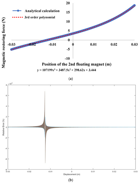
Figure 5.
(a) Magnetic restoring force of the 2nd floating magnet. (b) Relative errors of the fitting curves versus the analytical force.
Subsequently, the linear and nonlinear stiffness of these curves were determined. For the 2DOF oscillator system, the analytical measurements of the restoring forces were used to measure the linear and nonlinear stiffness of the system. The third-order polynomials were used to determine the linear and nonlinear stiffness of both floating magnets’ restoring forces. Figure 4a and Figure 5a show the analytical measurement of the magnetic restoring forces versus deflections of the floating magnets within the maximum deflection of 30 mm. Figure 4b and Figure 5b provide the relative error (%) in comparing the experimental data with analytical or predicted values over a range of displacement values. The sharp spike near zero displacement (around 0 m) in Figure 4b suggests that this region’s experimental force is very small or near zero. Since the denominator of the relative error formula is the experimental force, dividing by values near zero causes the relative error to explode, producing very large values. The symmetric “X” shape in Figure 4b around the origin indicates that this issue occurs for small positive and negative displacement values, which is typical in symmetric magnetic restoring force systems. In Figure 5b, around −0.012 m, the experimental force is nearly zero, causing the denominator in the formula to be very small. As a result, small absolute differences between the prediction and experiment produce huge percentage errors, hence the spike. The prediction model and experimental results align well across most displacement ranges. But at −0.012 m, there is a significant loss of reliability due to the near-zero experimental force, possible high sensitivity, noise in measurement, or the model not capturing certain behaviours accurately at that point.
5. Mathematical Model of the 2DOF Energy Harvester
When an external force is applied to a floating magnet or any floating magnet moves up and down, it creates an elastic restoring force in the magnetic spring. Figure 6 presents the free-body diagram of the SDOF magnetic spring-based energy harvester system.
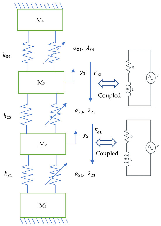
Figure 6.
Two-degrees-of-freedom magnetic spring-based energy harvester system.
The relative displacement of the first floating magnet is and the relative velocity and acceleration of the first floating magnet are and , respectively. Moreover, the relative displacement, velocity, and acceleration of the second floating magnet are ,, and , respectively. The magnetic flux density of the second magnet (first floating magnet) is and the total length of the first winding coil is . Similarly, the magnetic flux density of the third magnet (second floating magnet) is and the total length of the second winding coil is . The electromagnetic coupling coefficients are () and (). Moreover, and are the electromagnetic forces written as and , respectively.
The masses of the second (first floating magnet) and third (second floating magnet) magnets are M2 and M3, respectively. The damping force of the first floating magnet is and that of the second floating magnet is . In Figure 6, the linear stiffnesses are represented by , , and . The damping constants are represented by , , and . The nonlinear coefficients are presented by , , , and . In addition, the other nonlinear stiffnesses are , , and . In Figure 7, the linear stiffnesses are , , and . The damping constants , , and . The nonlinear coefficient is equal to . Moreover, and are equal to , and is equal to . In addition, the other nonlinear stiffnesses are ; ; and .
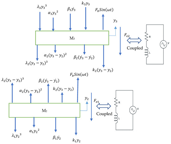
Figure 7.
Free-body diagram of the two-degrees-of-freedom system.
The dynamic equation of the motion of the system can be written as
Equation (10) can be expressed as
Equation (11) can be expressed as
6. Dynamic Analysis of the 2DOF Energy Harvester
The dynamics of the 2DOF energy harvester were analyzed by solving Equations (12)–(15) using linear and nonlinear stiffness, calculated from the magnetic restoring forces. The eigenvalues and frequency responses were first determined to understand the system. The diameter of the copper coil was 31 mm, and the number of turns of the winding coils was 100. The inside diameter and height of the winding coils were 75 mm and 10 mm, respectively. The total length of the winding coil was 23.5 m, and the inner resistance was 5.48 ohm. The average magnetic flux density we considered was 0.35 T (calculated from ANSYS MAXWELL version 2020 R2). Because of electromechanical coupling, the generator system consists of electrical and mechanical parts. Two winding coils were added outside the two floating magnets; therefore, the system has two resonance frequencies in the electrical part. Because of the two floating magnets, the system has two mechanical resonance frequencies. The electrical resonance frequencies did not change when changing the position of the floating magnets, but they changed when changing the total length of the winding coil (number of turns) and magnetic flux density. Moreover, the entire length of the winding coil does not affect the mechanical resonance frequency. All required parameters are presented in Table 1.

Table 1.
Required parameters.
The natural frequencies of the electrical parts were 953.46 rad/s and 948.77 rad/s when both floating magnets were in an equilibrium position. The natural frequencies for the mechanical parts were 44.17 rad/s and 33.75 rad/s. The natural frequencies of the mechanical part were almost similar for both generator systems with and without electrical–mechanical coupling. The imaginary parts of the eigenvalues (electrical parts) were zero, but the real parts were −953.47 and −948.78 in the equilibrium position. The eigenvalues of the mechanical part were −0.1954 ± 0.3962i (first floating magnet) and −0.2022 ± 0.2703i (second floating magnet) in the equilibrium position. The generator system’s frequency response in the equilibrium position is shown in Figure 8. Due to the electromechanical coupling, the frequency response graph does not show the peak amplitude.

Figure 8.
Frequency response of the generator system in the equilibrium position.
However, the peak resonance is shown to be at 40.1 rad/s. The generator system’s eigenvalues were analyzed by changing the floating magnets’ position. The frequency resonance was analyzed by connecting the external load or resistance parallel to the winding coils. Different external loads were connected to explore the frequency resonance of the generator system. The external load was varied from 500 ohms to 50,000 ohms to determine the resonance frequency. Figure 9 displays two resonances, and the values are 33 rad/s and 44.4 rad/s in the equilibrium position, which are almost similar to the natural frequencies of 44.17 rad/s and 33.75 rad/s without an external load, which were determined using eigenvalues. It can be seen in Figure 8 that the resonance frequency graph does not show the peak amplitude, but in Figure 9, the generator system with external load shows two peak resonant frequencies.
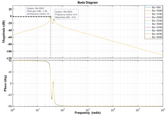
Figure 9.
Frequency response of the generator system with external load in the equilibrium position.
The natural frequencies of the mechanical parts were almost similar for both generator systems with and without external load. However, the natural frequencies of the electrical parts were much higher in the generator system with external load than in the system without external load. Compared to the generator system with or without external load, the system with external load showed better dynamic results.
The generator system’s displacements, velocities, and induced voltages were analyzed with an external force. If the external force was applied to any of the floating magnets or both floating magnets, then both floating magnets started moving relative to each other. Moreover, the velocity of the second floating magnet always remained higher than that of the first floating magnet. After adding the winding coils, the system was analyzed. Because of the movement of the floating magnets, the magnetic flux densities of the floating magnet cut the winding coils, which created an induced voltage inside the winding coils.
The applied external harmonic force (Fb) amplitude was 25 N, and the frequency (f) was 0.1 Hz. The values of linear stiffness, nonlinear stiffness, and damping constants are presented in Table 1. The state-space model equations were solved using the Ode23t solver in MATLAB (version R2020b) to find the system’s displacements, velocities, and induced voltages. Both floating magnets’ excitations were assumed to have initial displacements, and their corresponding velocities were zero. As expected, the displacements and the velocities were sinusoidal and 90° out of phase. At first, the generator system was analyzed by applying harmonic force to both floating magnets. Figure 10 presents the displacement and velocity of the first floating magnet, and Figure 11 displays the displacement and velocity of the second floating magnet.
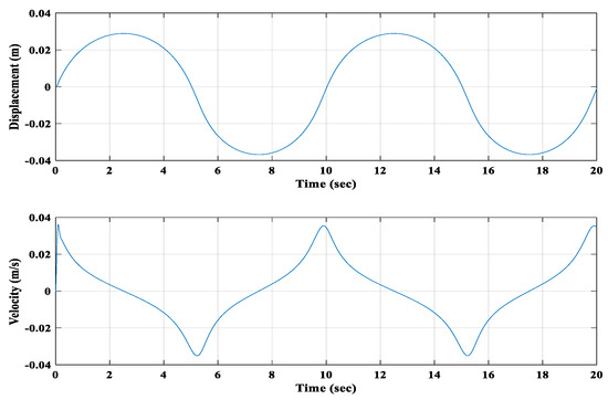
Figure 10.
Displacement and velocity of the 1st floating magnet.

Figure 11.
Displacement and velocity of the 2nd floating magnet.
Because of the applied harmonic force, the maximum displacement of the first floating magnet toward the second floating magnet was around 40 mm, and toward the bottom magnet, it was about 30 mm. The frequency of the applied harmonic force we considered was 0.1 Hz; therefore, Figure 10 shows two complete cycles. The maximum velocity of the first floating magnet was around 0.04 m/s. On the other hand, the maximum displacements of the second floating magnet toward the fourth (top fixed magnet) were around 50 mm and 40 mm towards the first floating magnet, as shown in Figure 11. The maximum velocity of the second floating magnet was around 0.05 m/s. For the same applied harmonic forces in both floating magnets, the second floating magnet achieved more displacement and velocity than the first floating magnet, as shown in Figure 12.

Figure 12.
Comparison of displacement and velocity of (a) 1st floating magnet and (b) 2nd floating magnet.
It was considered during the analysis that the first winding coil was placed outside of the first floating magnet, and the second winding coil was outside of the second floating magnet. The positions of both winding coils were not considered. As is known, due to the movement of the floating magnets, an induced voltage will be generated in the winding coil. The generated induced voltages were determined, as shown in Figure 13. The displacement and velocity of the second floating magnet were higher than those of the first floating magnet. Therefore, the second winding coil showed a higher induced voltage than the first. The maximum induced voltage in coil 2 was around 0.45 volts and in coil 1 was 0.3 volts. The generator system was analyzed by applying a harmonic force only on the second floating magnet. That applied harmonic force determined the displacements and velocities of both floating magnets.
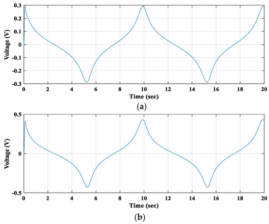
Figure 13.
Induced voltages in (a) 1st winding coil and (b) 2nd winding coil.
Moreover, the induced voltages for both coils were calculated. As the harmonic force was applied to the second floating magnet, the first floating magnet also started moving when the second floating magnet started moving. For this applied harmonic force (25 N amplitude), the second floating magnet achieved a higher displacement and velocity than the first. Figure 14 and Figure 15 present the displacement and velocity of the first and second floating magnets, respectively.
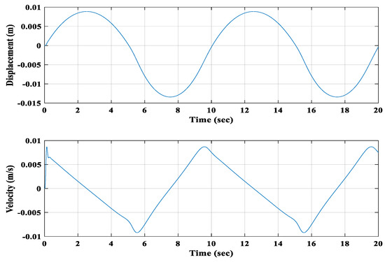
Figure 14.
Displacement and velocity of the 1st floating magnet.
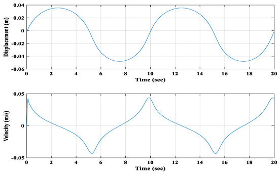
Figure 15.
Displacement and velocity of the 2nd floating magnet.
The first floating magnet moved 13 mm and 9 mm toward the second floating magnet and the first fixed magnet (bottom magnet), respectively. The maximum velocity was around 0.009 m/s during this movement. On the other hand, the second floating magnet moved 47 mm and 35 mm toward the top fixed magnet (fourth magnet) and the first floating magnet, respectively. The maximum velocity for the second floating magnet was around 0.045 m/s during this movement. Figure 16 compares the displacement and velocity of the first floating magnet with those of the second floating magnet. Figure 17 shows the induced voltages of both winding coils.
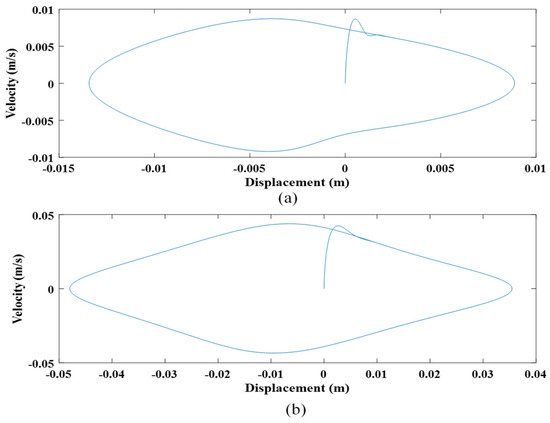
Figure 16.
Comparison of displacement and velocity of (a) 1st floating magnet and (b) 2nd floating magnet.
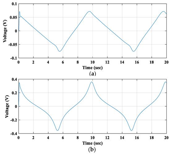
Figure 17.
Induced voltages in (a) 1st winding coil and (b) 2nd winding coil.
The relative displacements of both floating magnets were determined. The displacement and velocity of the second floating magnet were higher than those of the first floating magnet, as seen in Figure 16. Therefore, the induced voltage of coil 2 was higher than that of coil 1. The maximum induced voltage in coil 1 was around 0.075 volts and in coil 2 was 0.36 volts. Finally, the generator system was analyzed by applying the same harmonic force (25 N amplitude) only on the first floating magnet. As the harmonic force was applied on the first floating magnet, when the first floating magnet started moving, the second floating magnet also started moving. For this applied harmonic force (25 N amplitude), the second floating magnet achieved a higher displacement and velocity than the first floating magnet. Figure 18 and Figure 19 show the displacement and velocity of the first and second floating magnets, respectively.

Figure 18.
Displacement and velocity of the 1st floating magnet.
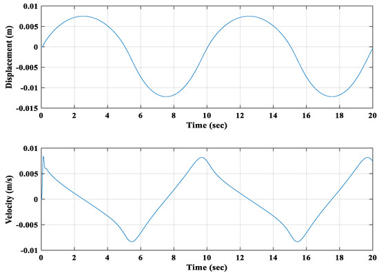
Figure 19.
Displacement and velocity of the 2nd floating magnet.
Due to the applied force, the first floating magnet moved 32 mm and 26 mm toward the second and first fixed magnet (bottom magnet), respectively. The calculated maximum velocity during that movement was around 0.027 m/s. On the other hand, the second floating magnet moved 12 mm toward the top fixed magnet (fourth magnet) and 7.5 mm toward the first floating magnet. The maximum velocity of the second floating magnet during that excitation was around 0.008 m/s. The second floating magnet achieved the highest displacement and velocity compared to the first floating magnet for this applied harmonic, as shown in Figure 20. Thus, the induced voltage of coil 1 was higher than that of coil 2. The maximum induced voltage in coil 2 was around 0.068 volts and in coil 1 was 0.22 volts, as can be seen in Figure 21.

Figure 20.
Comparison of displacement and velocity of (a) 1st floating magnet and (b) 2nd floating magnet.
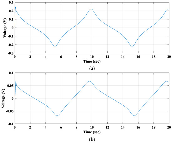
Figure 21.
Calculated induced voltages in (a) 1st winding coil and (b) 2nd winding coil.
Figure 22 and Figure 23 show the displacements and velocities of the first and second floating magnets when the force was applied on the first floating magnet and second floating magnet separately and both floating magnets simultaneously. Overall, the first floating magnet showed the minimum displacement and velocity during all different applications compared to the second floating magnet. Therefore, the first winding coil produced less induced voltage than the second. In Figure 22 and Figure 23, both floating magnets show the maximum displacement and velocity when the external force is applied on both floating magnets.


Figure 22.
Displacements of (a) 1st floating magnet and (b) 2nd floating magnet (note: FA = force applied; FM = floating magnet).


Figure 23.
Velocities of (a) 1st floating magnet and (b) 2nd floating magnet (note: FA = force applied; FM = floating magnet).
When the forces were applied on both floating magnets, both coils generated the maximum induced voltages compared to the other applied forces, as shown in Figure 24. Still, the second winding coil produced a higher induced voltage than the first winding coil. Hence, these theoretical analyses show that the 2DOF generator system can produce the maximum power if an external force is applied to both floating magnets.
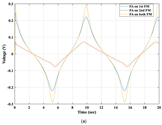
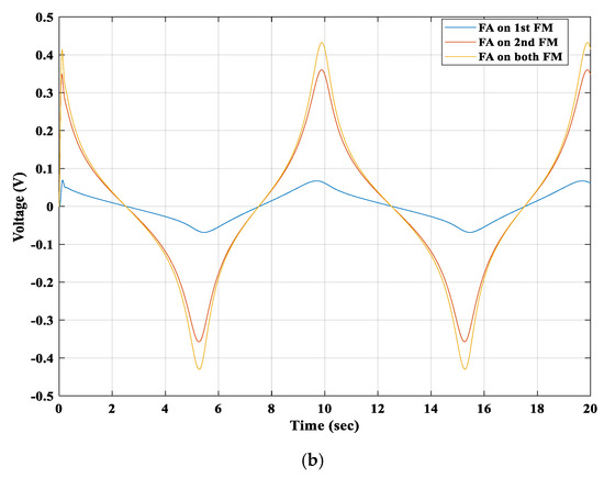
Figure 24.
Induced voltages of (a) 1st winding coil and (b) 2nd winding coil.
All analyses presented earlier had the amplitude and frequency of the applied force as 25 N and 0.1 Hz, respectively. The velocity of the floating magnet, magnetic flux density, number of turns of the winding coil, and applied external force can change the output-induced voltage of the magnetic spring-based generator system. By increasing the amplitude and frequency of the applied harmonic force, the output power of the 2DOF generator system can be increased. The 2DOF generator system was compared with the SDOF generator system. The amplitude and frequency of the applied harmonic force were 25 N and 0.1 Hz. A winding coil (100 turns) was considered for the SDOF-based generator system, and two winding coils (both 100 turns) were considered for the 2DOF generator system. Moreover, the same magnetic flux density and copper coil were considered when comparing both generator systems. The force was applied on both floating magnets and compared with the SDOF generator system. Figure 25 presents the comparison results of both generator systems.
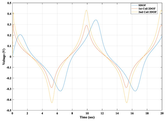
Figure 25.
Induced voltage when force was applied on both floating magnets in 2DOF system.
When the force was applied to both floating magnets, the generated induced voltage in coil 2 of the 2DOF generator system was higher than the generated induced voltage in coil 1. The generated voltage in coil 2 was higher than the generated induced voltage in the SDOF generator system. However, the voltage generated in coil 1 was almost similar to that generated in the SDOF system. Therefore, the 2DOF generator system is more efficient overall than the SDOF generator system.
7. Experimental Analysis
Sensor 1 was placed on top of the first magnet (fixed magnet), and sensor 2 was placed underneath the fourth magnet (top fixed magnet) to measure the displacement of the first and second floating magnets, respectively, as shown in Figure 1. Before starting the experimental work, all sensors were calibrated. The first and second winding coils were connected with the second and third ports of the data acquisition system. When the experimental setup was finalized, the sensors were powered.
Depending on the experimental design, fishing line was connected to either one floating magnet or both floating magnets. At first, the displacement of 1st floating magnet, which changed due to the changing position of the 2nd floating magnet, was calculated. The calculated displacement of the 1st floating magnet due to the movement of the 2nd floating magnet is presented in Figure 26. In Figure 26, the changing positions of both floating magnets toward the top and bottom magnets are represented by negative (−) and positive (+) signs, respectively. Figure 26 shows that when the 2nd floating magnet moved toward the top fixed magnet by 5 mm, the 1st floating magnet moved by 2 mm toward the 1st floating magnet. Similarly, the 1st magnet moved by 2 mm toward the bottom magnet, while the 2nd magnet moved toward the 1st floating magnet by 5 mm. Moreover, it can be seen from Figure 26 that for every 5 mm movement of the 2nd floating magnet, the 1st floating magnet moved by 2 mm. For the experimental investigation, the projected amplitude and frequency of the harmonic force were 15 N and 3.88 Hz, respectively. To create the harmonic force, an ABB servo motor was used. The experiment was conducted for a few minutes, during which time all signal data from sensors 1 and 2, as well as the winding coils, were collected using a data acquisition system. All collected data were analyzed using MATLAB, and a low-pass filter was applied to obtain a smooth graph.
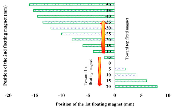
Figure 26.
Position of the 1st floating magnet vs. position of the 2nd floating magnet.
The same amplitude and frequency of the harmonic force were applied in the analytical model and compared with the experimental results. Figure 27 displays the displacement and velocity of the 1st floating magnet, and Figure 28 shows the displacement and velocity of the 2nd floating magnet. The blue and green lines in Figure 27 and Figure 28 represent analytical and experimental measurements, respectively. During the analytical investigation, the 1st floating magnet moved toward the bottom magnet by about 17 mm and toward the 2nd floating magnet by around 21 mm, as presented by the blue line in Figure 27a. The 1st floating magnet moved toward the 2nd floating magnet by 12 mm and toward the bottom by around 25 mm during the experimental analysis, as shown by the green line in Figure 27a.

Figure 27.
(a) Displacement and (b) velocity of the 1st floating magnet (FM: floating magnet).

Figure 28.
(a) Displacement and (b) velocity of the 2nd floating magnet (FM: floating magnet).
On the other hand, the 2nd floating magnet moved toward the 1st floating magnet by about 34 mm and toward the top magnet by around 40 mm during the analytical analysis, as presented by the blue line in Figure 28a. The 2nd floating magnet moved toward the top magnet by 38 mm and toward the 1st floating magnet by around 34 mm during the experiment, as shown by the green line in Figure 28a. The 1st floating magnet moved up and down with an average velocity of 0.09 m/s during the experiment and 0.085 m/s during the analytical analysis, as presented in Figure 27b. On the other hand, the 2nd floating magnet moved up and down with an average velocity of 0.093 m/s during the analytical analysis and 0.094 m/s during the experiment, as presented in Figure 28b. Figure 29 presents the induced voltage of the energy harvester.

Figure 29.
Induced voltages in (a) 1st winding coil and (b) 2nd winding coil (WC: winding coil).
The blue and green lines in Figure 29 represent the induced voltage of the analytical and experimental measurements, respectively. In Figure 29, the induced voltage of the generator for the analysis is compared with that of the experiment. The average maximum induced voltage in winding coil 1 was 3.5 V for the analysis and 5 V for the experiment. On the other hand, the average maximum induced voltage in winding coil 2 was 7.2 V for the analytical analysis and 7 V for the experiment. Figure 27, Figure 28 and Figure 29 show that the experimental model is well validated with the analytical model.
8. Conclusions
This study proposed and analysed a two-degrees-of-freedom (2DOF) magnetic spring-based electromagnetic energy harvester through an integrated approach combining analytical modelling, numerical simulation, prototyping, and experimental validation. The dual-floating-magnet configuration enabled the system to harness two resonant modes, offering a broader frequency bandwidth and increased energy-harvesting potential compared to single-degree-of-freedom (SDOF) designs. The nonlinear magnetic restoring forces were modelled using fitted polynomials, and system dynamics were solved using the state-space approach in MATLAB with the ODE23t solver, chosen for its capacity to handle moderately stiff electromechanical systems. Analytical results for induced voltage and system response were compared against experimental measurements, showing good agreement in both waveform and amplitude trends, with peak-induced voltages reaching approximately 7.2 V (analytical) and 7.0 V (experimental) under 15 N excitation.
While the model demonstrated strong predictive capability, certain discrepancies remain between the simulated and experimental results. These differences are attributed to idealised assumptions in the modelling process—such as the perfect alignment of magnetic components, neglect of minor frictions, uniform magnetic field distribution, and simplified coil dynamics—which are challenging to replicate precisely in physical prototypes. These assumptions introduce uncertainty, especially under high displacement or nonlinear regimes, and highlight the scope for further refinement.
Future work will aim for the following objectives:
- Improve the modelling of magnetic interactions through more accurate finite element- or machine learning-assisted characterisation.
- Incorporate real-world effects such as friction, misalignment, and coil saturation.
- Optimise circuit load configurations for efficient power conditioning.
Despite its limitations, the proposed system confirms that 2DOF magnetic spring-based architectures are promising for broadband, low-frequency vibration energy harvesting. This work contributes both a robust modelling framework and valuable experimental validation, laying a foundation for more advanced and scalable harvester designs.
Author Contributions
Conceptualization, R.A., I.H. and K.M.; methodology, R.A. and K.M.; software, R.A.; validation, R.A.; formal analysis, R.A.; investigation, R.A.; resources, R.A.; data curation, R.A.; writing—original draft preparation, R.A.; writing—review and editing, I.H. and K.M.; visualization, R.A. and K.M.; supervision, I.H. and K.M.; project administration, K.M.; funding acquisition, K.M. All authors have read and agreed to the published version of the manuscript.
Funding
This research received no external funding.
Institutional Review Board Statement
Not applicable.
Informed Consent Statement
Not applicable.
Data Availability Statement
The data presented in this article are available on request from the corresponding author.
Acknowledgments
The authors gratefully acknowledge the Australian Government Research Training Program Scholarship for Raju Ahamed’s study at Curtin University, Australia.
Conflicts of Interest
The authors declare no conflicts of interest.
References
- Wang, G.; Zheng, Y.; Zhu, Q.; Liu, Z.; Zhou, S. Asymmetric tristable energy harvester with a compressible and rotatable magnet-spring oscillating system for energy harvesting enhancement. J. Sound Vib. 2023, 543, 117384. [Google Scholar] [CrossRef]
- Kim, H.; Kim, S.; Xue, K.; Seok, J. Modeling and performance analysis of electromagnetic energy harvester based on torsional galloping phenomenon. Mech. Syst. Signal Process. 2023, 195, 110287. [Google Scholar] [CrossRef]
- Rosso, M.; Corigliano, A.; Ardito, R. Numerical and experimental evaluation of the magnetic interaction for frequency up-conversion in piezoelectric vibration energy harvesters. Meccanica 2022, 57, 1139–1154. [Google Scholar] [CrossRef]
- Rosso, M.; Ardito, R. A review of nonlinear mechanisms for frequency up-conversion in energy harvesting. Actuators 2023, 12, 456. [Google Scholar] [CrossRef]
- Rosso, M.; Cuccurullo, S.; Perli, F.P.; Maspero, F.; Corigliano, A.; Ardito, R. A method to enhance the nonlinear magnetic plucking for vibration energy harvesters. Meccanica 2024, 59, 1577–1592. [Google Scholar] [CrossRef]
- Yan, Y.; Zhang, Q.; Han, J.; Wang, W.; Wang, T.; Cao, X.; Hao, S. Design and investigation of a quad-stable piezoelectric vibration energy harvester by using geometric nonlinearity of springs. J. Sound Vib. 2023, 547, 117484. [Google Scholar] [CrossRef]
- Ju, Y.; Li, Y.; Tan, J.; Zhao, Z.; Wang, G. Transition mechanism and dynamic behaviors of a multi-stable piezoelectric energy harvester with magnetic interaction. J. Sound Vib. 2021, 501, 116074. [Google Scholar] [CrossRef]
- Debnath, B.; Kumar, R. A comparative simulation study of the different variations of PZT piezoelectric material by using a MEMS vibration energy harvester. IEEE Trans. Ind. Appl. 2022, 58, 3901–3908. [Google Scholar] [CrossRef]
- Chen, L.; Ma, Y.; Hou, C.; Su, X.; Li, H. Modeling and analysis of dual modules cantilever-based electrostatic energy harvester with stoppers. Appl. Math. Model. 2023, 116, 350–371. [Google Scholar] [CrossRef]
- Ahamed, R.; Howard, I.; McKee, K. Dynamic analysis of magnetic spring-based nonlinear oscillator system. Nonlinear Dyn. 2023, 111, 15705–15736. [Google Scholar] [CrossRef]
- Li, J.Y.; Zhang, T.; Lun, M.M.; Zhang, Y.; Chen, L.Z.; Fu, D.W. Facile control of ferroelectricity driven by ingenious interaction engineering. Small 2023, 19, 2301364. [Google Scholar] [CrossRef] [PubMed]
- Beeby, S.P.; Wang, L.; Zhu, D.; Weddell, A.S.; Merrett, G.V.; Stark, B.; Szarka, G.; Al-Hashimi, B.M. A comparison of power output from linear and nonlinear kinetic energy harvesters using real vibration data. Smart Mater. Struct. 2013, 22, 075022. [Google Scholar] [CrossRef]
- Owens, B.A.; Mann, B.P. Linear and nonlinear electromagnetic coupling models in vibration-based energy harvesting. J. Sound Vib. 2012, 331, 922–937. [Google Scholar] [CrossRef]
- Saravia, C.M.; Ramírez, J.M.; Gatti, C.D. A hybrid numerical-analytical approach for modeling levitation based vibration energy harvesters. Sens. Actuators A Phys. 2017, 257, 20–29. [Google Scholar] [CrossRef]
- Masoumi, M.; Wang, Y. Repulsive magnetic levitation-based ocean wave energy harvester with variable resonance: Modeling, simulation and experiment. J. Sound Vib. 2016, 381, 192–205. [Google Scholar] [CrossRef]
- Dos Santos, M.P.S.; Ferreira, J.A.; Simões, J.A.; Pascoal, R.; Torrão, J.; Xue, X.; Furlani, E.P. Magnetic levitation-based electromagnetic energy harvesting: A semi-analytical non-linear model for energy transduction. Sci. Rep. 2016, 6, 18579. [Google Scholar] [CrossRef]
- Carneiro, P.; dos Santos, M.P.S.; Rodrigues, A.; Ferreira, J.A.; Simões, J.A.; Marques, A.T.; Kholkin, A.L. Electromagnetic energy harvesting using magnetic levitation architectures: A review. Appl. Energy 2020, 260, 114191. [Google Scholar] [CrossRef]
- Fan, K.; Zhang, Y.; Liu, H.; Cai, M.; Tan, Q. A nonlinear two-degree-of-freedom electromagnetic energy harvester for ultra-low frequency vibrations and human body motions. Renew. Energy 2019, 138, 292–302. [Google Scholar] [CrossRef]
- Monaco, M.L.; Russo, C.; Somà, A. Numerical and experimental performance study of two-degrees-of-freedom electromagnetic energy harvesters. Energy Convers. Manag. X 2023, 18, 100348. [Google Scholar] [CrossRef]
- Zhang, R.; Wang, X.; Shu, H.; John, S. The effects of the electro-mechanical coupling and Halbach magnet pattern on energy harvesting performance of a two degree of freedom electromagnetic vibration energy harvester. Int. J. Veh. Noise Vib. 2018, 14, 124–146. [Google Scholar] [CrossRef]
- Mukhopadhyay, S.; Donaldson, J.; Sengupta, G.; Yamada, S.; Chakraborty, C.; Kacprzak, D. Fabrication of a repulsive-type magnetic bearing using a novel arrangement of permanent magnets for vertical-rotor suspension. IEEE Trans. Magn. 2003, 39, 3220–3222. [Google Scholar] [CrossRef]
- Liu, H.; Gudla, S.; Hassani, F.A.; Heng, C.H.; Lian, Y.; Lee, C. Investigation of the nonlinear electromagnetic energy harvesters from hand shaking. IEEE Sens. J. 2014, 15, 2356–2364. [Google Scholar] [CrossRef]
- Ahamed, R.; Howard, I.; McKee, K. Study of gravitational force effects, magnetic restoring forces, and coefficients of the magnetic spring-based nonlinear oscillator system. IEEE Trans. Magn. 2022, 58, 9200618. [Google Scholar] [CrossRef]
Disclaimer/Publisher’s Note: The statements, opinions and data contained in all publications are solely those of the individual author(s) and contributor(s) and not of MDPI and/or the editor(s). MDPI and/or the editor(s) disclaim responsibility for any injury to people or property resulting from any ideas, methods, instructions or products referred to in the content. |
© 2025 by the authors. Licensee MDPI, Basel, Switzerland. This article is an open access article distributed under the terms and conditions of the Creative Commons Attribution (CC BY) license (https://creativecommons.org/licenses/by/4.0/).