Hybrid Improved PSO Algorithm for Soil Property Parameter Estimation

Abstract

This study proposes a hybrid PSO-EDO algorithm, integrating Particle Swarm Optimization (PSO) and the Exponential Distribution Optimizer (EDO) for efficient and accurate estimation of soil property parameters. The proposed algorithm combines the strengths of Standard PSO (SPSO) and the Exponential Distribution Optimizer (EDO). Three key innovations are introduced: (1) SPM chaotic mapping enhances initial population diversity; (2) dynamic inertia weight balances global exploration and local exploitation; (3) the memoryless property of EDO improves escape capability from local optima. Benchmark tests demonstrate that PSO-EDO achieves near-theoretical optimal convergence errors (mean error ≤ 10⁻¹⁶ for unimodal functions such as F1 and F2) and reduces the computation time by 14.5% compared to EDO. For multimodal functions (e.g., F3), PSO-EDO significantly outperforms PSO-WOA (Particle Swarm Optimization-Whale Optimization Algorithm) with a 22.3% reduction in error. Simulation experiments further validate its engineering practicality: in soil parameter estimation, PSO-EDO completes 1000 iterations in just 1.95 s, with key parameters (e.g., sinkage coefficient n) controlled within a 7.32% error margin. This provides an efficient solution for real-time traversability assessment of autonomous vehicles on soft terrains.

1. Introduction

In recent years, there has been a notable increase in the prevalence of special engineering vehicles designed for use on unpaved roads, off-road vehicles, and agricultural vehicles [1,2]. This has led to a corresponding rise in the number of vehicles that are required to operate on soft ground. The low bearing capacity and poor traction of soft ground present a significant challenge for vehicles, often impeding their ability to move. Consequently, the study of soil parameter estimation has become a crucial aspect of assessing potential hazardous driving areas and enabling the use of unmanned vehicles in such environments.

Terrain mechanics are crucial for solving the problem of vehicle mobility on soft ground, with researchers investigating the relationship between wheel subsidence and interaction forces by creating a semi-empirical model. Bekker [3] systematically studied the fundamental theory of terrain–vehicle mechanics and proposed formulas for calculating wheel sinkage and compression resistance. Wong (2001) and Reece (1965) [4,5] improved Bekker’s formulas based on experimental data, while Janosi [6] proposed a formula to represent shear stress distribution. These formulas involve soil and empirical parameters, and the model requires efficient and accurate estimation of soil parameters through inverse prediction.

Hybrid PSO methods have been extensively studied for parameter optimization. Early works integrated PSO with other evolutionary algorithms: Yin et al. [7] combined PSO, GA, and neural networks (PSO-GA-BP) for forest fire prediction, while Song et al. [8] proposed PSO-ACO for energy scheduling. Bansal et al. [9] further introduced PSO-WOA to address high-dimensional convergence issues. Recent advancements demonstrate broader applicability. In microseismic source localization, Han et al. [10] developed a PSO-GA algorithm with dynamic learning factors, achieving 59% higher accuracy than GA. For medical hyperthermia, Ji et al. [11] utilized stochastic PSO (SPSO) to minimize thermal damage through adaptive laser parameter tuning. In computer vision, Zhang et al. [12] proposed SPSO-Pruner for YOLOv5 network pruning, reducing the parameters by 50% with an improved F1-score. Multi-objective frameworks also emerged: Uzer and Inan [13] combined WOA, PSO, and Lévy flight (WOALFVWPSO), outperforming benchmarks in 19/23 functions, while Bansal and Aggarwal [9] applied PSO-WOA to cloud–fog workflows, reducing execution cost by 18%.

Despite the significant potential of these hybrid PSO algorithms (e.g., PSO-WOA and GA-PSO) across diverse domains, they still face core challenges in convergence efficiency, computational cost, and local optima avoidance. The existing methods exhibit critical trade-offs—PSO-GA-BP [7] and WOALFVWPSO require manual parameter tuning, while SPSO-Pruner and PSO-WOA struggle with scalability in high-dimensional spaces. Specifically, PSO-WOA suffers from insufficient convergence speed in high-dimensional optimization due to static parameter configurations, and PSO-GA is prone to local optima entrapment in multimodal problems owing to fixed crossover and mutation rates; moreover, complex adaptation rules further amplify computational burdens. To address these limitations, this paper proposes a novel hybrid algorithm, PSO-EDO (Particle Swarm Optimization-Exponential Distribution Optimizer), which integrates dynamic inertia weight adjustment for adaptive exploration–exploitation balance, leverages the memoryless property of the Exponential Distribution Optimizer (EDO) [14] to prevent premature convergence, and employs SPM chaotic mapping to enhance initial population diversity. Compared to recent studies (e.g., PSO-WOA in cloud–fog scheduling and PSO-GA in microseismic source localization), PSO-EDO eliminates the need for complex parameter tuning, ensures computational efficiency, significantly improves global search capability by reducing local optima risks, and provides an advanced solution for real-time engineering applications.

2. Off-Road Wheel–Soil Interaction Force Model

Before estimating soil parameters, it is necessary to explore the mechanical relationship between the wheel and the soil. Figure 1 depicts Wong’s semi-empirical model [4], with the parameters defined in

Table 1. Wong’s semi-empirical model of wheel–soil interaction.

Symbol	Definition	Unit
$\theta$	The angle formed between the line connecting any point on the contact surface to the wheel center and the vertical direction, serving as the independent variable in theoretical integration calculations	rad
${\theta }_1$	The angle between the line connecting the front contact point of the tire–soil interface to the wheel center and the vertical direction	rad
${\theta }_2$	The angle formed between the line connecting the rear contact point of the tire–soil interface to the wheel center and the vertical direction	rad
${\theta }_m$	The angular position on the contact surface where the normal stress reaches its peak value	rad
$z$	The vertical deformation of soil at the front contact point of the tire–soil interface	m
$z_2$	The vertical deformation of soil at the rear contact point of the tire–soil interface	m
$r$	Wheel radius	m
$T$	Wheel torque	N·m
$F_{DP}$	Traction force	N
${\tau }_1$	$\mathrm{Normal} \mathrm{stress} \mathrm{at} {\theta }_1$	kPa
${\tau }_2$	$\mathrm{Normal} \mathrm{stress} \mathrm{at} {\theta }_2$	kPa
${\sigma }_1$	$\mathrm{Shear} \mathrm{stress} \mathrm{at} {\theta }_1$	kPa
${\sigma }_2$	$\mathrm{Shear} \mathrm{stress} \mathrm{at} {\theta }_2$	kPa

. Empirical models are commonly used in research because they balance model precision with reduced research difficulty. Based on Dr. Bekker’s findings [3], the static sinkage $z_0$ can be expressed by Equation (1):

$$z_0={\left[{\displaystyle \frac{3W}{b\left(3-n\right)\left(\frac{k_c}{b}+k_{\phi }\right)\sqrt{D}}}\right]}^{⌊{\displaystyle \frac{2}{\left(2n+1\right)}}⌋}$$

(1)

In the equation, W represents the vertical wheel load (in newtons, N), b denotes the wheel width (in meters, m), and $k_c$, $k_{\phi }$, and n refer to the soil cohesion modulus (kPa·m⁻ⁿ), the soil friction angle modulus (kPa·m⁻ⁿ), and the soil sinkage coefficient (dimensionless), respectively. The term $D$ represents the wheel diameter (in meters, m), defined as twice the radius ($D=2r$), where $r$ is the wheel radius. As indicated by the equation, $z_0$ reflects only the static sinkage resulting from wheel–soil interaction, without accounting for the dynamic sinkage caused by wheel slip. Researcher Reece [5] further highlighted the significance of dynamic sinkage in his study, emphasizing its dependence on slip ratio and transient soil behavior. To capture the dynamic sinkage component, Lopez-Arreguin [2] proposed a modified sinkage exponent n that incorporates the dynamic effect:

$$n=n_0+n_{1}s$$

(2)

where $n_0$ is the constant value obtained from direct soil testing, $n_1$ is the fitting constant, and s is the slip ratio.

Regarding the normal stress at the contact surface between a rigid wheel and the soil, Bekker expressed it using the following equation:

$$\sigma =\left({\displaystyle \frac{k_c}{b}}+k_{\phi }\right)z^n$$

(3)

Since the theoretical determination of the maximum stress point is not well established, Wong [4] used an empirical equation to determine this point:

$$\left\{\begin{array}{c}{\theta }_m={\theta }_1\left(C_1+C_{2}s\right)\\ {\theta }_2={C_3\theta }_1\end{array}\right.$$

(4)

where $C_1$, $C_2$, and $C_3$ are coefficients obtained from fitting experimental data. These coefficients can be adjusted iteratively to improve the curve fitting. However, to reduce computational complexity and enhance efficiency, some researchers have conducted studies on these three values. Ding [15] found that the ${\theta }_2$ obtained through visual methods may be larger than the calculated ${\theta }_2$. Since ${\theta }_2$ is much smaller than ${\theta }_1$, the stress in the region from ${\theta }_2$ to 0 degrees is minimal, leading some researchers to consider ${\theta }_2$ as approximately 0. Du [16] studied the three coefficients in scenarios where experiments or simulations are not feasible, providing suitable values. He found that the predicted results align well with the fitted model when $C_1=0.5$ and $C_2=C_3=0$.

According to the geometric relationship, the equations relating $z_0$ and ${\theta }_1$ in Figure 1 are given as (5) and (6):

$$z_0=r\left(1-cos{\theta }_1\right)$$

(5)

$${\theta }_1=\mathit{arccos}\left(1-{\displaystyle \frac{z_0}{r}}\right)$$

(6)

By combining Equations (1), (3) and (5), and for the sake of computational convenience, $C_3$ is set to 0, leading to the following equation:

$$\left\{\begin{array}{c}{\sigma }_1\left(\theta \right)=\left({\displaystyle \frac{k_c}{b}}+k_{\phi }\right){r^n(cos\theta -cos{\theta }_1)}^n ({\theta }_m\le \theta \le {\theta }_1)\\ {\sigma }_2\left(\theta \right)=\left({\displaystyle \frac{k_c}{b}}+k_{\phi }\right)r^n{\left[cos\left({\theta }_1-\theta \left({\displaystyle \frac{1}{C_1+C_{2}s}}-1\right)\right)-cos{\theta }_1\right]}^n \left(0\le \theta \le {\theta }_m\right) \end{array}\right.$$

(7)

The magnitude of shear stress between the wheel and the soil depends on the shear deformation of the soil. The relationship between shear stress and soil deformation can be expressed using Janosi’s simplified formula [6]:

$$\tau =\left(c+\sigma tan\phi \right)\left(1-e^{-{\displaystyle \frac{j}{k}}}\right)$$

(8)

The shear displacement of the soil, $j$ [4] is as follows:

$$j\left(\theta \right)=r\left[\left({\theta }_1-\theta \right)-\left(1-s\right)\left(sin{\theta }_1-sin\theta \right)\right]$$

(9)

By combining Equations (7)–(9), in the active region from ${\theta }_m$ to ${\theta }_1$:

$${\tau }_1=\left(c+{\sigma }_1\left(\theta \right)tan\phi \right)\left(1-e^{-{\displaystyle \frac{r\left[\right({\theta }_1-\theta )-(1-s\left)\right(sin{\theta }_1-sin\theta \left)\right]}{k}}}\right)$$

(10)

In the active region from 0 to ${\theta }_m$:

$${\tau }_2=\left(c+{\sigma }_2\left(\theta \right)tan\phi \right)\times \left(1-e^{-{\displaystyle \frac{r\left[\right({\theta }_1-\theta )-(1-s\left)\right(sin{\theta }_1-sin\theta \left)\right]}{k}}}\right)$$

(11)

From the mechanical equilibrium of the soil and the analysis of soil stress, it can be concluded that:

$$W=rb\left[{\int }_0^{{\theta }_m}{\sigma }_2\left(\theta \right)cos\theta d\theta +{\int }_{{\theta }_m}^{{\theta }_1}{\sigma }_1\left(\theta \right)cos\theta d\theta +{\int }_0^{{\theta }_m}{\tau }_2\left(\theta \right)sin\theta d\theta +{\int }_{{\theta }_m}^{{\theta }_1}{\tau }_1\left(\theta \right)sin\theta d\theta \right]$$

(12)

$$F_{DP}=rb\left[{\int }_0^{{\theta }_m}{\tau }_2\left(\theta \right)cos\theta d\theta +{\int }_{{\theta }_m}^{{\theta }_1}{\tau }_1\left(\theta \right)cos\theta d\theta -{\int }_0^{{\theta }_m}{\sigma }_2\left(\theta \right)sin\theta d\theta -{\int }_{{\theta }_m}^{{\theta }_1}{\sigma }_1\left(\theta \right)sin\theta d\theta \right]$$

(13)

$$T=r^{2}b\left[{\int }_0^{{\theta }_m}{\tau }_2\left(\theta \right)d\theta +{\int }_{{\theta }_m}^{{\theta }_1}{\tau }_1\left(\theta \right)d\theta \right]$$

(14)

Performing calculations for Equations (12)–(14) using computational tools is highly complex and not suitable for real-time applications. To address this issue, the three equations were simplified. Simpson’s Rule, represented by Equation (15), is a numerical integration method that approximates the definite integral by using quadratic polynomials to fit the integrand. Its accuracy is relatively high because it takes into account the behavior of the integrand over the interval, not just the values at the endpoints.

$${\int }_a^{b}f\left(x\right)dx={\displaystyle \frac{b-a}{6}}\left[f\left(a\right)+4f\left({\displaystyle \frac{a+b}{2}}\right)+f\left(b\right)\right]$$

(15)

By substituting Equation (15) into Equations (12)–(14), the following mathematical model can be established:

$$\left\{\begin{array}{c}{f}_1\left(W,s,c,\phi ,n,k_c,k_{\phi },K,{\theta }_1\right)=0\\ f_2\left(F_{DP},s,c,\phi ,n,k_c,k_{\phi },K,{\theta }_1\right)=0\\ f_3\left(T,s,c,\phi ,n,k_c,k_{\phi },K,{\theta }_1\right)=0\end{array}\right.$$

(16)

The mathematical model (16) consists of three nonlinear equations. Therefore, solving for the soil parameters can be transformed into the problem of selecting an appropriate method to estimate the parameters of the nonlinear model.

3. Improvement of the PSO Algorithm

3.1. Traditional PSO Algorithm

Particle Swarm Optimization (PSO) [17] is an evolutionary computation technique proposed by Dr. Eberhart and Dr. Kennedy in 1995. The algorithm has garnered significant attention for its simplicity and minimal control parameters. The idea of PSO is inspired by the foraging behavior of bird flocks, where the birds are abstracted into particles. Each particle’s position represents a solution, and the process of solving the problem within the search space simulates the way birds share information to find the best food source.

Assume the search space of the particle swarm has D dimensions, and the total number of particles is N. The position of the $i^{th}$ particle is defined as follows:

$$X_i=\left[X_{i1},X_{i2},X_{i3},\dots ,X_{iD}\right],$$

and its velocity as follows:

$$V_i=\left[V_{i1},V_{i2},V_{i3},\dots ,V_{iD}\right].$$

The current position of the $i^{th}$ particle is represented by:

$$P_i=\left[P_{i1},P_{i2},P_{i3},\dots \dots ,P_{iD}\right].$$

The PSO algorithm begins by randomly initializing the position $X_i$ and velocity $V_i$ for each particle. At each iteration, the historical best position of each particle is updated as follows:

$${Pbest}_i=\left[{Pbest}_{i1},{Pbest}_{i2},{Pbest}_{i3},\dots \dots ,{Pbest}_{iD}\right],$$

while the global best position of the entire swarm is as follows:

$${Gbest}_i=\left[{Gbest}_{i1},{Gbest}_{i2},{Gbest}_{i3},\dots \dots ,{Gbest}_{iD}\right],$$

The position and velocity of each particle are then updated using the following equations:

$$\left\{\begin{array}{c}{V}_{ij}^{k+1}=\omega V_{ij}^k+c_1{r}_1\left(P_{ij}-X_{ij}^k\right)+c_2{r}_2\left(G_{ij}-X_{ij}^k\right)\\ X_{ij}^{k+1}=X_{ij}^k+V_{ij}^{k+1}\end{array}\right.$$

(17)

where $k$ denotes the current iteration, $\omega$ is the inertia weight, $c_1$ and $c_2$ are acceleration coefficients, and $r_1$ and $r_2$ are random numbers uniformly distributed in [0, 1].

3.2. Improvement Strategies for the PSO Algorithm

PSO has global search capability, but it may still fall into local optima when dealing with complex multimodal functions. This occurs because particles may converge near local optimal points, limiting their ability to explore beyond a certain range. Improvements to the algorithm can mitigate these limitations to some extent. From the structural perspective of the PSO algorithm, common improvement methods [18] include modifying the inertia weight, adjusting learning factors, updating particle positions and velocities, and integrating other algorithms.

Abdel-Basset et al. [14] proposed a novel population-based metaheuristic algorithm called the Exponential Distribution Optimizer (EDO) based on the exponential probability distribution model. Due to the memoryless property of the exponential distribution, the algorithm can ignore and discard the historical states of particles, as past failures are independent and have no impact on future outcomes. Even unsuccessful particles can contribute to generating new solutions in subsequent updates. This approach reduces the probability of the algorithm becoming trapped in local optima.

Therefore, the improvement strategy in this paper focuses on reducing the likelihood of becoming trapped in local optima. First, the population is initialized using SPM chaotic mapping. Then, an adaptive inertia weight is introduced based on the fitness value during iterations, enhancing the algorithm’s ability to explore a larger search space in the early stages and perform precise searches around the optimal solution in the later stages. Finally, the idea of the EDO algorithm is incorporated into the PSO algorithm to increase the randomness of particle position updates, thereby improving the accuracy of the enhanced algorithm.

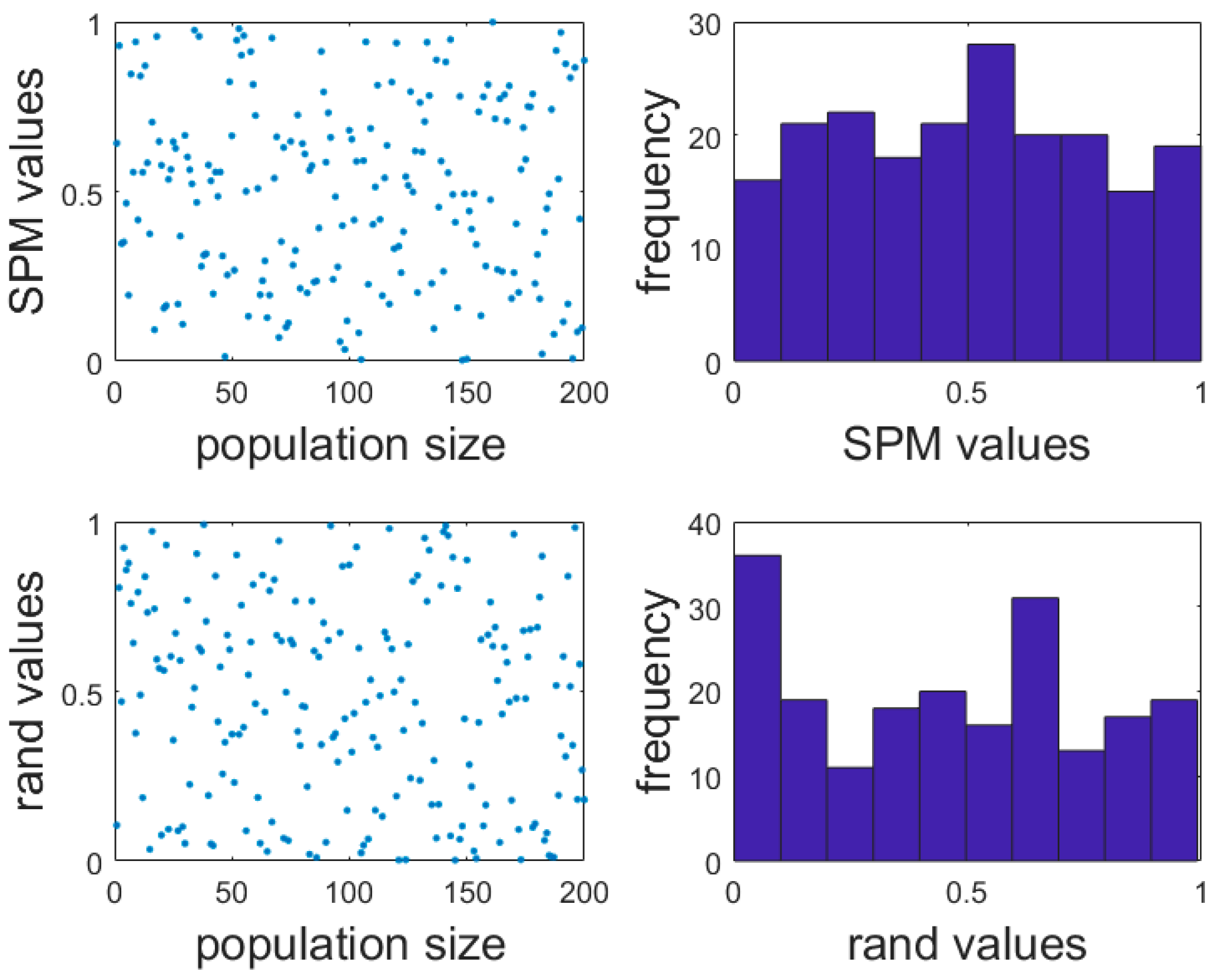
3.3. Improvement in Initialization of Positions

In the PSO algorithm, the random function rand is typically used to initialize the initial positions and velocities of the particle swarm. While this method significantly enhances the randomness of particles, it is challenging to ensure the uniformity of particles across the search space, making it easier for particles to become trapped in local optima and affecting the convergence accuracy of the algorithm. Chaotic mapping [19] is a mathematical model widely applied in nonlinear dynamical systems, characterized by high irregularity and pseudo-randomness. The SPM chaotic mapping (Equation (18)) is selected for initialization due to its superior ergodicity and computational efficiency, as demonstrated in image encryption studies [20]. By combining Sine and PWLCM mappings, the SPM map expands the chaotic range while ensuring full traversal of the search space, with its piecewise function design effectively avoiding particle aggregation in local regions (as shown in Figure 2). Experimental tests with parameters $\eta =0.4$ and $\mu =0.3$ maximize the Lyapunov exponent (≈0.5), enhancing chaotic behavior. Furthermore, compared to hyper-chaotic systems, SPM reduces computational complexity by 58% while maintaining equivalent security, making it particularly suitable for high-dimensional optimization problems where both efficiency and robustness are critical. Chaotic initialization can also reduce the sensitivity of the algorithm to the initial parameter settings. Equation (18) provides the SPM chaotic sequence:

$$x\left(i+1\right)=\left\{\begin{array}{c}mod\left({\displaystyle \frac{x\left(i\right)}{\eta }}+\mu sin\left(\pi x\left(i\right)\right)+r,1\right) 0\le x\left(i\right)<\eta \\ mod\left({\displaystyle \frac{x\left(i\right)/\eta }{0.5-\eta }}+\mu sin\left(\pi x\left(i\right)\right)+r,1\right) \eta \le x\left(i\right)<0.5 \\ mod\left({\displaystyle \frac{1-x\left(i\right)/\eta }{0.5-\eta }}+\mu sin\left(\pi (1-x\left(i\right))\right)+r,1\right) 0.5\le x\left(i\right)<1-\eta \\ mod\left({\displaystyle \frac{1-x\left(i\right)}{0.5-\eta }}+\mu sin\left(\pi (1-x\left(i\right))\right)+r,1\right) 1-\eta \le x\left(i\right)<1 \end{array}\right.$$

(18)

where $mod(a,b)$ denotes the remainder of $a/b$, and $r$ is a random number between 0 and 1. The experimental results indicate that when $\eta =0.4$ and $\mu =0.3$, the sequence generated by the SPM mapping exhibits better ergodicity and randomness, with the chaotic orbit values in the range of [0, 1]. Figure 2 illustrates the distribution and frequency histograms of SPM sequences and random sequences with an overall size of 200, exhibiting values between 0 and 1. It can be observed that the SPM sequence values are more evenly distributed.

3.4. Inertia Weight of the PSO Algorithm

The inertia weight $\omega$ determines how much influence the particle’s velocity has on the velocity in the next iteration. There are two types of inertia weight mechanisms: static and dynamic. When the inertia weight is set to a relatively large value, the swarm exhibits strong global search capability in the early stages of iteration but low convergence precision in the later stages. On the other hand, with a smaller inertia weight, the search capability is weaker initially, but the convergence precision improves in later stages. As a result, static inertia weight fails to meet the PSO requirements for both fast search speed and high precision. In their research, Shi and Eberhart [21] found that using an inertia weight of 0.9 at the beginning of the PSO process and gradually reducing it to 0.4 by the end yields better performance. They used the number of iterations as the basis for adjusting the inertia weight, as shown in Equation (19):

$$\omega \left(t\right)=\left({\omega }_{max}-{\omega }_{min}\right)\left({\displaystyle \frac{K-k}{K}}\right)+{\omega }_{min}$$

(19)

where $K$ represents the maximum number of iterations, and $k$ denotes the current iteration. In this method, if the algorithm converges quickly, the inertia weight may differ significantly from 0.4 during the convergence phase. Conversely, if the algorithm converges slowly, the inertia weight may decrease too early, potentially affecting the final accuracy. Therefore, in this paper, fitness is used as the evaluation metric, and the improved formula is presented as in Equation (20):

$$\omega ={\omega }_{min}+({\omega }_{max}-{\omega }_{min})\times {\displaystyle \frac{{fit}_k}{{fit}_1}}$$

(20)

In the equation, ${\omega }_{max}$ and ${\omega }_{min}$ denote the maximum and minimum values of the inertia weight, respectively. ${fit}_1$ is the fitness value at the first iteration, and ${fit}_k$ is the fitness value at the $k^{th}$ iteration.

3.5. Improvement in Position Update

In the EDO algorithm, two matrices, X and Y, are constructed. Matrix X stores the historical best positions of all particles, while matrix Y stores the newly generated positions of the particles. To simulate the memoryless property, changes in the positions in Y do not need to consider the corresponding values in X. Before updating the position of particle $i$, a random number ${\alpha }_i$ is generated using a random number generator, where ${\alpha }_i$ lies within the range of [0, 1]. If ${\alpha }_i<0.5$, the position of particle $i$ is updated according to Equations (21)–(24):

$$v_i=\left\{\begin{array}{c}a\left(y_i^k-{\sigma }^2\right)+b{x}_{guide}^k if x_i^k=y_i^k \\ b\left(y_i^k-{\sigma }^2\right)+log\left(\phi \right){\ast x}_i^k else \end{array}\right.$$

(21)

$$\left\{\begin{array}{c}a=f^{10}\\ b=f^5\\ f=2\ast rand\left( \right)-1\end{array}\right.$$

(22)

$$\sigma ={\displaystyle \frac{x_i^k+y_i^k}{2}}$$

(23)

$$x_{guide}^k={\displaystyle \frac{x_1^k+x_2^k+x_3^k}{3}}$$

(24)

where $v_i$ represents the updated position of particle $i$; $\sigma$ denotes the standard deviation; $x_i^k$ is the historical best position of particle $i$ during the $k^{th}$ iteration, and $y_i^k$ is the position of particle $i$ during the $k^{th}$ iteration. $x_{guide}^k$ denotes the guiding solution of the swarm at the $k^{th}$ iteration, where $x_1^k$ is the optimal solution, $x_2^k$ is the second-best solution, and $x_3^k$ is the third-best solution of the population at the $k^{th}$ iteration. rand() represents a random number in the range [0, 1], and $\phi$ also denotes a random number within the range [0, 1].

If ${\alpha }_i\ge 0.5$, the particle swarm updates its position using the PSO algorithm. Since the PSO algorithm converges quickly, it enhances the computational speed of the overall algorithm. The updated formula is provided in Equation (25):

$${\displaystyle \genfrac{}{}{0pt}{}{V_i^{k+1}=\omega V_i^k+c_1{r}_1\left(P_i-X_i^k\right)+c_2{r}_2\left(G_i-X_i^k\right)}{v_i^{k+1}=X_i^k+V_i^{k+1}}}$$

(25)

The PSO-EDO proposed in this study operates on the physical principle of randomly dividing the particle swarm into two subgroups: an EDO optimization subgroup and a PSO optimization subgroup. The EDO subgroup conducts its search based on the memoryless property of exponential distribution. For instance, in a discrete solution space (e.g., four possible directions: up, down, left, right), if a particle has moved left ten consecutive times, the probability of moving right in the next step remains 25%, completely independent of its historical trajectory. Meanwhile, the PSO subgroup achieves rapid convergence through inertia preservation, individual best (pbest), and global best (gbest) guidance mechanisms, thereby enhancing computational efficiency. After each iteration, particles that previously belonged to the PSO subgroup and may have become trapped in local optima have a chance to be randomly reassigned to the EDO subgroup in the subsequent iteration. This reassignment leverages the memoryless property to facilitate escape from local optima.

In summary, the pseudocode for the PSO-EDO computational process is as follows (Algorithm 1):

Algorithm 1. Computational Process of the PSO-EDO Algorithm
01	Set the maximum number of iterations K, the number of particles N, and the upper $U_b$ and lower $L_b$ bounds of the particle positions and the dimensions D of the fitness function.
02	Initialize the population based on SPM chaotic mapping.
03	Initialize the population X, compute the fitness of each individual, and sort them.
04	Initialize the memoryless matrix Y as Y = X.
05	for $k=1:K$
06	Identify the top three optimal individuals and compute the guiding solution $x_{guide}^k$ using Equation (24).
07	Calculate $a$, $b$, $f$, and σ using Equations (22) and (23).
08	for $i=1:N$
09	if $\alpha <0.5$
10	Update the position using Equation (21).
11	else
12	Update the position using Equation (25).
13	end if
14	${\mathit{Y}}_{\mathit{i}}={\mathit{V}}_{\mathit{i}}$
15	if $cost\left({\mathit{Y}}_{\mathit{i}}\right)<cost\left({\mathit{X}}_{\mathit{i}}\right)$
16	${\mathit{X}}_{\mathit{i}}={\mathit{Y}}_{\mathit{i}}$
17	end if
18	end for
19	Re-sort based on the fitness of the particle positions in matrix $\mathit{X}$.
20	end for
21	Output the average optimal value, optimal value, standard deviation, and average computation time.

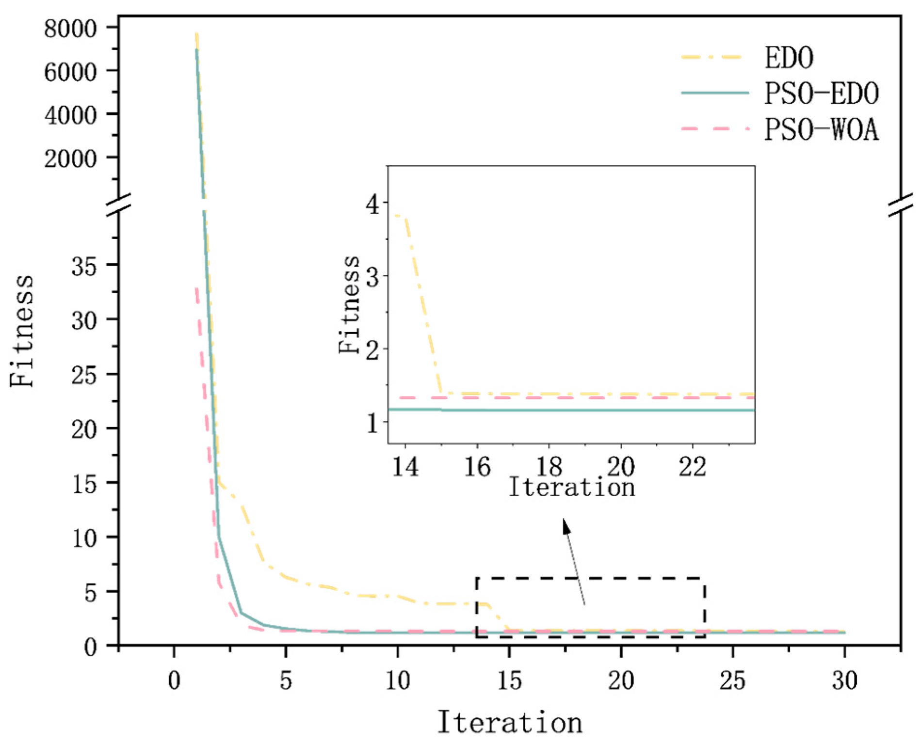
3.6. Comparative Test Experiment

To validate the performance of the PSO-EDO, we selected six widely-used benchmark test functions (F1–F6) from the 2017 IEEE Congress on Evolutionary Computation (IEEE CEC) [22], as shown in

Table 2. Benchmark functions.

Function	Range	Dimension	Optimal Value
$F_1\left(x\right)=x_1^2+{10}^6{\displaystyle \sum _{i=2}^D}{x}_i^2$	$\left[-\mathrm{10,10}\right]$	30	0
$F_2\left(x\right)={\displaystyle \sum _{i=1}^D}{\left|x_i\right|}^{i+1}$	$\left[-\mathrm{100,100}\right]$	30	0
$F_3\left(x\right)={\displaystyle \sum _{i=1}^{D-1}}\left[100{\left(x_i^2-x_{i+1}\right)}^2+{\left(x_i^2-1\right)}^2\right]$	$\left[-\mathrm{10,10}\right]$	30	0
$F_4\left(x\right)=-20e^{-0.2\sqrt{{\displaystyle \frac{1}{D}}\sum _{i=1}^D{x}_i^2}}-e^{{\displaystyle \frac{1}{D}}\sum _{i=1}^D\cos \left(2\pi x_i\right)}+20+e$	$\left[-\mathrm{32,32}\right]$	30	0
$F_5\left(x\right)={\displaystyle \sum _{i=1}^D}\left[x_i^2-10\cos \left(2\pi x_i\right)+10\right]$	$\left[-\mathrm{5.12,5.12}\right]$	30	0
$F_6\left(x\right)={\displaystyle \frac{1}{4000}}{\displaystyle \sum _{i=1}^D}{x}_i^2-{\displaystyle \prod _{i=1}^D}cos\left({\displaystyle \frac{x_i}{\sqrt{i}}}\right)+1$	$\left[-\mathrm{600,600}\right]$	30	0

. These functions, encompassing both unimodal and multimodal types, are designed to evaluate the algorithm’s performance across diverse optimization scenarios. While standard test functions are commonly employed in algorithm comparisons, their selection here is intentional and grounded in the specific challenges of soil parameter estimation, particularly for multivariate, high-dimensional, nonlinear, and multimodal optimization problems. For example, F1 and F2, as classical unimodal functions, simulate idealized conditions in soil parameter optimization where a single global optimum exists, such as estimating parameters like cohesion modulus ($k_c$) under homogeneous soil conditions. In contrast, F3–F6, as multimodal functions, emulate complex real-world scenarios where soil parameters (e.g., soil friction angle ($\phi$) and sinkage coefficient ($n$) may exhibit multiple local optima depending on soil heterogeneity, necessitating the algorithm to avoid premature convergence. By optimizing these standard functions, we comprehensively assess PSO-EDO’s global search capability, ability to escape local optima, and computational efficiency in addressing intricate soil parameter estimation challenges.

Figure 3 shows the plots of F1–F6 for the two-dimensional case. Six related algorithms were selected for comparative experiments: basic PSO [23], SPSO, PSO-GA, PSO-WOA, EDO, and the improved PSO algorithm. To ensure fairness, the basic parameters of the different PSO algorithms and the improved PSO algorithm were kept consistent, including the population size $N=30$, the dimensionality $D=30$, and the maximum number of iterations $k_{max}$ = 1000. Each algorithm was run independently 30 times, and the mean, best value, standard deviation (std), and computation time of the optimal results were calculated as performance metrics for algorithm optimization.

From

Table 3. The optimization results of the comparative testing experiment.

Function	Performance Metrics	PSO	SPSO	PSO-GA	PSO-WOA	EDO	PSO-EDO
F1	Mean	46.6667	18.4343	1.9908 × 108	779.8416	0	0
	Best	2.5343 × 10−7	0.0585	6.9623 × 107	0.0537	0	0
	Std	50.7416	38.0227	4.8996 × 107	869.0725	0	0
	Time (s)	0.1930	0.1904	0.2640	0.1445	0.3424	0.2043
F2	Mean	6.7014 × 1034	3.3667 × 1032	6.9615 × 1042	5.92 × 104	0	0
	Best	1.0001 × 1014	1887.8	1.0061 × 1034	6.46 × 10−10	0	0
	Std	2.5362 × 1035	1.8252 × 1033	2.5332 × 1043	3.18 × 105	0	0
	Time (s)	0.3217	0.3005	0.3639	0.2461	0.4775	0.3178
F3	Mean	726.5842	105.8248	2.6968 × 105	1.0566	29	23.4577
	Best	16.6368	17.8986	8.9816 × 104	2.03 × 10−4	29	0.1445
	Std	2.5265 × 103	195.028	1.2390 × 105	1.2549	0	5.8286
	Time (s)	1.5197	1.483	1.5197	1.3997	1.5758	1.4501
F4	Mean	2.1070	0.094	18.3392	0.0744	8.8818 × 10−16	8.8818 × 10−16
	Best	3.2920 × 10−11	0.0013	16.0595	2.59 × 10−4	8.8818 × 10−16	8.8818 × 10−16
	Std	1.6360	0.3153	0.9442	0.058	0	0
	Time (s)	0.2049	0.2164	0.2867	0.1869	0.4092	0.2431
F5	Mean	106.7421	45.9901	300.5527	0.6695	0	0
	Best	53.7277	21.8909	245.1119	7.44 × 10−5	0	0
	Std	33.7884	14.8105	27.1314	2.3247	0	0
	Time (s)	0.2174	0.2243	0.2872	0.1638	0.4060	0.2425
F6	Mean	0.1170	0.012	198.0842	0.3537	0	0
	Best	0	6.83 × 10−5	136.4232	0.0105	0	0
	Std	0.1870	0.0121	44.3387	0.2968	0	0
	Time (s)	1.5253	1.413	1.5829	1.4101	1.6735	1.4597

, it can be observed that the mean and standard deviation of the PSO-EDO optimization results for F1 and F2 reach the theoretical optimal values. This result indicates that the improved algorithm offers good solution accuracy and stability for these unimodal optimization problems. Although the EDO algorithm also achieved the theoretical optimal values for the mean and standard deviation in F1 and F2, its average computation time was longer than that of PSO-EDO. The PSO-WOA algorithm also yielded good optimal values in the 30 iterations; however, its mean optimal value and standard deviation were relatively high, indicating low stability.

For the multimodal problems F4, F5, and F6, the optimization results of EDO and PSO-EDO were similar, both achieving the theoretical optimal values. However, the improved algorithm was 0.1 to 0.2 s faster on average than EDO in terms of computation time. The PSO-WOA algorithm also produced desirable optimization results with a relatively short average computation time, but its robustness was inferior to the improved algorithm.

The PSO and SPSO algorithms performed similarly to the PSO-WOA algorithm for F4 and F6, but their optimization performance for F5 was not satisfactory. For the F3 test, the PSO-WOA algorithm achieved the best optimization result, followed by PSO-EDO and EDO, indicating that the improved algorithm possesses better capability to escape from local optima compared to PSO and EDO. Although PSO-WOA performed well for F3, it was far inferior to PSO-EDO for other functions.

In the tests on unimodal functions F1 and F2, the computational time difference between the PSO and PSO-EDO was not significant. However, PSO-EDO demonstrated superior stability, with a standard deviation of 0, indicating that the algorithm consistently converges precisely to the global optimal solution in every run. For multimodal functions F4 and F5, the computational efficiency of the standard PSO algorithm was within 15.5%, faster than that of PSO-EDO. In contrast, for functions F3 and F6, the computational time of PSO-EDO was reduced by up to 4.6% compared to PSO. From a performance metric perspective, PSO-EDO significantly outperforms the standard PSO algorithm in terms of mean error, best value, and standard deviation, with its optimization results nearly attaining the theoretical optimal values. Notably, in optimization problems with highly volatile solution spaces (e.g., function F2), the performance of the standard PSO algorithm degraded substantially, exhibiting a standard deviation as high as $2.5\times {10}^{35}$. In stark contrast, PSO-EDO maintained a stable standard deviation of 0, unequivocally validating the superiority and robustness of the improved algorithm in solving complex optimization problems.

In summary, compared to PSO, SPSO, PSO-GA, and PSO-WOA, the PSO-EDO algorithm significantly improves convergence accuracy. Compared to the EDO algorithm, it reduces computation time and enhances the ability to escape from local optima.

Figure 4 shows the average fitness curves of different algorithms during the iterative evolution of the F1–F6 test functions, providing a more intuitive comparison of the convergence speed and accuracy of the algorithms. As observed in Figure 4 for F2, F4, and F5, the convergence speed of PSO-EDO is significantly better than that of other algorithms.

Table 4. The mean F1–F6 fitness evolution curves by using PSO-EDO in 30 independent runs.

Iteration	F1	F2	F3	F4	F5	F6
1	6.39 × 108	4.58 × 1051	2.93 × 106	20.67	443.87	610.03
2	1.18 × 108	1.74 × 1047	3.31 × 105	7.84	123.95	305.93
3	1.72 × 107	2.09 × 1045	9.03 × 104	4.24	26.41	128.03
4	8471.73	3.02 × 1039	1007.56	2.01	1.65	115.90
5	362.42	9.04 × 1030	32.21	1.32	0.02	75.45
6	13.47	3.49 × 1027	23.72	0.15	0.00	46.28
7	0.03	2.23 × 1020	24.16	0.00	0.00	40.38
8	0.00	7.92 × 108	23.86	0.00	0.00	45.85
9	0.00	0.00	24.01	0.00	0.00	38.42
10	0.00	0.00	24.00	0.00	0.00	0.23
11	0.00	0.00	23.73	0.00	0.00	0.00
12	0.00	0.00	23.76	0.00	0.00	0.00
13	0.00	0.00	23.57	0.00	0.00	0.00
14	0.00	0.00	23.71	0.00	0.00	0.18
15	0.00	0.00	23.87	0.00	0.00	0.08

presents the average fitness of the PSO-EDO algorithm over the first 15 iterations for the F1–F6 test functions, showing that the improved algorithm nearly completes convergence within the first 10 generations. Although other algorithms, except for PSO-GA, also exhibit relatively fast convergence for F1, F3, and F6, their performance is still inferior to that of the improved algorithm.

To further verify the statistical significance of the performance differences among algorithms, Wilcoxon signed-rank tests were performed between PSO-EDO and the other four comparison algorithms (PSO, SPSO, PSO-GA, and PSO-WOA) based on the fitness data presented in

Table 5. Wilcoxon signed-rank test results for fitness comparison.

Comparison Groups	Test Statistic	p-Value	Significance Conclusion
PSO-EDO vs. PSO	0.0	$<0.001\left(\approx 3.33\times {10}^{-165}\right)$	Significant difference
PSO-EDO vs. SPSO	271.0	$<0.001\left(\approx 7.50\times {10}^{-165}\right)$	Significant difference
PSO-EDO vs. PSO-GA	226,060.0	$<0.01\left(\approx 0.0081\right)$	Significant difference
PSO-EDO vs. PSO-WOA	15,510.0	$<0.001\left(\approx 1.32\times {10}^{-145}\right)$	Significant difference

. The results show that all pairwise comparisons yielded p-values of less than 0.01, indicating that the performance improvements achieved by PSO-EDO are statistically significant. These differences are unlikely to be caused by random fluctuations, thereby reinforcing the robustness and effectiveness of the proposed method.

4. Simulation Results and Discussion

4.1. Simulation Results

Based on the established soil property parameter estimation model, simulation experiments were conducted using MATLAB R2020a version. The simulation data were obtained from [24], and the true values of the corresponding vehicle parameters and soil properties are listed in

Table 6. Vehicle parameters and experimental soil characteristic parameters.

Category	Vehicle		Parameters for Terrain
Symbol	r	b	K	KP	c	n	φ
Unit	m	m	m	kPa$·$m−n	kPa	-	$°$
Value	0.2	0.1	0.025	1532.4	1	1.1	30
Source	Direct Measurement		Plate Penetration Test	Calculated as $KP={\displaystyle \frac{k_c}{b}}+k_{\phi }$	Triaxial Test	Empirical Fitting	Direct Shear Test

.

Among the four types of PSO algorithms, the PSO-WOA algorithm achieved better optimization results, and the performance of the EDO algorithm was similar to that of the improved algorithm. Therefore, PSO-WOA, EDO, and PSO-EDO algorithms were selected for simulation comparison.

Table 7. Simulation results of three algorithms.

Function	Performance Metrics	K [m]	KP [kPa·m−n]	c [kPa]	n	φ [°]	Time [s]
EDO	Global Best	0.0232	1620.54	1.0267	1.345	29.46	2.2803
	Mean Best	0.0232	1620.54	1.0267	1.345	30.85
	Mean Error	7.32%	5.75%	2.67%	22.27%	2.81%
PSO-EDO	Global Best	0.0232	1620.54	1.0267	1.345	30.85	1.9487
	Mean Best	0.0232	1620.54	1.0267	1.345	30.85
	Mean Error	7.32%	5.75%	2.67%	22.27%	2.81%
PSO-WOA	Global Best	0.0232	1620.54	1.0267	1.345	30.85	2.3773
	Mean Best	0.0232	1620.54	1.0267	1.345	30.85
	Mean Error	7.32%	5.75%	2.67%	22.27%	2.81%

presents the simulation results of the improved algorithm, with a maximum of 1000 iterations and 30 independent runs. Global Best refers to the set of values with the lowest fitness among the 30 optimization results, Mean Best represents the mean of the optimal values (0) across the 30 runs, and Mean Error denotes the error rate between the mean value and the true value.

As shown in the table, after 30 simulations, the parameter estimation results for the three algorithms are identical, with no significant differences. The only difference lies in the average computation time: PSO-EDO has the shortest computation time, followed by the EDO algorithm, with the PSO-WOA algorithm taking the longest.

Figure 5 shows the average fitness over the first 30 iterations for the simulation results of the three algorithms. As observed in Figure 5, both the PSO-WOA and PSO-EDO algorithms converge within the first 10 iterations, while the EDO algorithm takes until the 15th iteration to complete convergence. This indicates that the EDO algorithm has a slower convergence speed during the simulation compared to the other two algorithms.

4.2. Discussion

First, the simulation results in Table 7 show that the error rate of the improved algorithm is kept within 10%. The average computation time of the PSO-EDO algorithm is 14.5% shorter than that of the EDO algorithm and 18.0% shorter than that of the PSO-WOA algorithm. Second, as observed in Figure 5, although the improved algorithm has a relatively high fitness in the early iterations, its convergence speed is close to that of the PSO-WOA algorithm, with convergence nearly completed within 10 iterations. In terms of fitness at convergence, the PSO-EDO algorithm achieves a lower fitness value compared to the other two algorithms.

From the above, the following conclusions can be drawn: In the parameter estimation simulation, the improved algorithm reduces the computation time compared to the other two algorithms without sacrificing computational accuracy or convergence speed. After completing the iterations, it achieves a lower fitness value, demonstrating that the PSO-EDO algorithm offers higher precision and convergence speed. The performance improvement of the algorithm lies in combining the strengths of the EDO and PSO algorithms. The EDO algorithm introduces higher randomness during the exploration phase, reducing the risk of becoming trapped in local optima. Meanwhile, the PSO algorithm offers faster convergence, and dynamically adjusting the inertia weight using Equation (20) enhances convergence speed, reduces computation time, and improves accuracy.

In the study of soil property parameter estimation, optimizing complex mathematical models is often required. Improving computation speed while maintaining accuracy shortens the research cycle and facilitates real-time acquisition of soil property data. In the fields of artificial intelligence and logistics, faster computation translates into savings in computing resources, energy, and human resources. Therefore, this research holds significant practical value.

In summary, applying the PSO-EDO algorithm to soil property parameter estimation successfully achieves efficient and accurate parameter estimation, and the simulation results validate the feasibility of this method.

However, some limitations and application challenges should be acknowledged. First, although the algorithm performs well under the tested conditions, its estimation accuracy may degrade in highly heterogeneous or moisture-sensitive soils, where the underlying physical parameters exhibit strong nonlinearity or spatial variability. Second, the scalability of the PSO-EDO algorithm in large-scale, high-resolution terrain datasets remains to be validated, as increased data dimensionality and volume may impose additional computational burdens and memory requirements.

Moreover, the current validation is based on simulation data under idealized conditions, which may not fully capture the complexity of real-world environments. In field applications, factors such as sensor noise, incomplete data, and dynamic terrain changes can influence algorithm performance. Additionally, actual terrain conditions often involve irregular profiles and variable soil–vehicle interactions that are difficult to model precisely. Therefore, future research should focus on validating the PSO-EDO algorithm using field data, exploring its integration with onboard systems for real-time soil parameter estimation, and evaluating its robustness under varying environmental conditions.

5. Conclusions

This paper proposes a soil property parameter estimation method based on the integration of a wheel–soil mechanical model with the PSO-EDO algorithm. First, the mechanical interaction between the wheel and soil was analyzed, and a wheel–soil model was developed using calculus, followed by the simplification of the governing equations. Next, SPM chaotic mapping was introduced for population initialization, and the inertia weight was updated based on the fitness values during the iterative process. Subsequently, the strengths of the EDO and SPSO algorithms were combined to develop the improved PSO-EDO algorithm. The performance of the proposed algorithm was tested using common benchmark functions and compared with basic PSO, SPSO, PSO-GA, PSO-WOA, and EDO algorithms. The experimental results indicate that the PSO-EDO algorithm performs well for both unimodal and multimodal functions. Although its computation speed is slightly slower, it achieves higher accuracy.

In the soil property parameter estimation simulation, the PSO-WOA, EDO, and PSO-EDO algorithms, which performed well in the benchmark function tests, were compared. The PSO-EDO algorithm’s average computation time was 1.9487 s, 18.0% shorter than that of the PSO-WOA algorithm and 14.5% shorter than that of the EDO algorithm. The PSO-EDO and PSO-WOA algorithms showed similar convergence speeds, both completing convergence within 10 iterations, approximately five generations faster than the EDO algorithm. The error rate for soil property parameter estimation was generally within 10%, indicating good performance and demonstrating the feasibility and superiority of the proposed method. In future work, the structure of the PSO-EDO algorithm needs to be further refined to enhance its performance.

Despite these promising results, several limitations should be acknowledged. First, the current validation is based on simulation data under idealized conditions. In real-world applications, data noise, missing values, and heterogeneous soil conditions may affect performance. Second, the algorithm’s scalability for large-scale or high-dimensional terrain data remains to be further tested.

Future work should aim to: (1) validate the algorithm with field-collected data in diverse environments; (2) extend the method to accommodate various complex soil types and dynamic terrain characteristics; and (3) explore the integration of deep learning or hybrid intelligent systems to further enhance estimation accuracy, robustness, and computational efficiency.

References

1. Lyasko, M. Slip sinkage effect in soil–vehicle mechanics. J. Terramech. 2010, 47, 21–31. [Google Scholar] [CrossRef]
2. Lopez-Arreguin, A.J.R.; Gundlach, B.; Stoll, E. Do lunar rover wheels sink equally on Earth and Moon? Results Phys. 2019, 15, 102617. [Google Scholar] [CrossRef]
3. Bekker, M.G. Theory of Land Locomotion: The Mechanics of Vehicle Mobility; University of Michigan Press: Ann Arbor, MI, USA, 1956. [Google Scholar]
4. Wong, J.Y. Theory of Ground Vehicles; Wiley-Interscience: Hoboken, NJ, USA, 2001. [Google Scholar]
5. Reece, A.R. Principles of soil-vehicle mechanics. Proc. Inst. Mech. Eng. 1965, 180, 45–66. [Google Scholar] [CrossRef]
6. Janosi, Z.; Hanamoto, B. The analytical determination of drawbar pull as a function of slip for tracked vehicle in deformable soils. In Mechanics of Soil-Vehicle Systems: Proceedings of the 1st International Conference on the Mechanics of Soil-Vehicle Systems; Edizioni Minerva Tecnica: Torino, Italy, 1961; Volume 41. [Google Scholar]
7. Yin, Z.; Wang, F.; Tang, T.; Luo, Q.; Xiang, K. The forest fire prediction in JiangXi province based on PSO-GA-BP neural network. In Proceedings of the 2nd Workshop on Advanced Research and Technology in Industry Applications (WARTIA 2016), Dalian, China, 14–15 May 2016; Atlantis Press: Dordrecht, The Netherlands, 2016. [Google Scholar]
8. Song, Q.; Yu, L.; Li, S.; Hanajima, N.; Zhang, X.; Pu, R.; Rajamohan, V. A Review of Intelligent Ground Vehicle Technologies. Int. J. Intell. Syst. 2023, 2023, 1–20. [Google Scholar]
9. Bansal, S.; Aggarwal, H. A multiobjective optimization of task workflow scheduling using hybridization of PSO and WOA algorithms in cloud-fog computing. Cluster Comput. 2024, 27, 10921–10952. [Google Scholar] [CrossRef]
10. Zhu, H.; Ding, Y. Optimized Dynamic Collision Avoidance Algorithm for USV Path Planning. Sensors 2023, 23, 4567. [Google Scholar] [CrossRef] [PubMed]
11. Zhao, D.; Lei, Z.; An, C. Research on battery thermal management system based on liquid cooling plate with honeycomb-like flow channel. Appl. Therm. Eng. 2023, 218, 119324. [Google Scholar] [CrossRef]
12. Zhang, Y.; Liu, X.; Chen, Y.; Xie, L.; Wang, H.; Salem, O. SPSO-Pruner: A Network Pruning Method on YOLOv5 for Fewer Categories Scenarios. Neural Process. Lett. 2023, 55, 789–812. [Google Scholar] [CrossRef]
13. Uzer, M.S.; Inan, O. Application of improved hybrid whale optimization algorithm to optimization problems. Neural Comput. Appl. 2023, 35, 12345–12360. [Google Scholar] [CrossRef]
14. Abdel-Basset, M.; El-Shahat, D.; Jameel, M.; Abouhawwash, M. Exponential distribution optimizer (EDO): A novel math-inspired algorithm for global optimization and engineering problems. Artif. Intell. Rev. 2023, 56, 9329–9400. [Google Scholar] [CrossRef]
15. Ding, L.; Deng, Z.; Gao, H.; Tao, J.; Iagnemma, K.D.; Liu, G. Interaction mechanics model for rigid driving wheels of planetary rovers moving on sandy terrain with consideration of multiple physical effects. J. Field Robot. 2014, 32, 827–859. [Google Scholar] [CrossRef]
16. Du, Y.; Gao, J.; Jiang, L.; Zhang, Y. Development and numerical validation of an improved prediction model for wheel-soil interaction under multiple operating conditions. J. Terramech. 2018, 79, 1–21. [Google Scholar] [CrossRef]
17. Kennedy, J.; Eberhart, R.C. Particle swarm optimization. In Proceedings of the ICNN’95—IEEE International Conference on Neural Networks (ICNN), Perth, Australia, 27 November–1 December 1995. [Google Scholar]
18. Shami, T.M.; El-Saleh, A.A.; Alswaitti, M.; Al-Tashi, Q.; Summakieh, M.A.; Mirjalili, S. Particle swarm optimization: A comprehensive survey. IEEE Access 2022, 10, 10031–10061. [Google Scholar] [CrossRef]
19. Altay, E.V.; Alatas, B. Bird swarm algorithms with chaotic mapping. Artif. Intell. Rev. 2019, 53, 1373–1414. [Google Scholar] [CrossRef]
20. Ban, D.H.; Lü, X.; Wang, X.Y. Computer Science; Hohai University: Nanjing, China, 2019. [Google Scholar]
21. Shi, Y.; Eberhart, R.C. Empirical study of particle swarm optimization. In Proceedings of the 1999 Congress on Evolutionary Computation (CEC 1999), Washington, DC, USA, 6–9 July 1999. [Google Scholar]
22. Wu, G.; Mallipeddi, R.; Suganthan, P.N. Problem Definitions and Evaluation Criteria for the CEC 2017 Competition on Constrained Real-Parameter Optimization; Technical Report; National University of Defense Technology: Changsha, China, 2017. [Google Scholar]
23. Eberhart, R.; Kennedy, J. A new optimizer using particle swarm theory. In Proceedings of the Sixth International Symposium on Micro Machine and Human Science (MHS’95), Nagoya, Japan, 4–6 October 1995. [Google Scholar]
24. Sun, D.-B.; Di, Y.-Q.; Cui, H.-H. A real-time vehicle-terramechanics model for visual simulation. In Proceedings of the International Conference on Materials Engineering and Information Technology Applications (MEITA 2015), Guilin, China, 30–31 August 2015. [Google Scholar]
Figure 1. Wong’s semi-empirical model of wheel–soil interaction.
Applsci 15 04451 g001
Figure 2. The discrete distribution plot and frequency histogram of SPM sequences and random sequences.
Applsci 15 04451 g002
Figure 3. F1–F6 benchmark test function three-dimensional diagram.
Applsci 15 04451 g003
Figure 4. The mean F1–F6 fitness evolution curves by using PSO, SPSO, PSO-GA, PSO-WOA, EDO, and PSO-EDO in 30 independent runs.
Applsci 15 04451 g004
Figure 5. Fitness line graph for the first 30 iterations of the three algorithms.
Applsci 15 04451 g005