EPIIC: Edge-Preserving Method Increasing Nuclei Clarity for Compression Artifacts Removal in Whole-Slide Histopathological Images

Abstract

Hematoxylin and eosin (HE) staining is widely used in medical diagnosis. Stained slides provide crucial information to diagnose or monitor the progress of many diseases. Due to the large size of scanned images of whole tissues, a JPEG algorithm is commonly used for compression. This lossy compression method introduces artifacts visible as 8 × 8 pixel blocks and reduces overall quality, which may negatively impact further analysis. We propose a fully unsupervised Edge-Preserving method Increasing nucleI Clarity (EPIIC) for removing compression artifacts from whole-slide HE-stained images. The method is introduced in two versions, EPIIC and EPIIC Sobel, composed of stain deconvolution, gradient-based edge map estimation, and weighted smoothing. The performance of the method was evaluated using two image quality measures, $PSNR$ and $SSIM$, and various datasets, including BreCaHAD with HE-stained histopathological images and five other natural image datasets, and compared with other edge-preserving filtering methods and a deep learning-based solution. The impact of compression artifacts removal on the nuclei segmentation task was tested using Hover-Net and STARDIST models. The proposed methods led to improved image quality in histopathological and natural images and better segmentation of cell nuclei compared to other edge-preserving filtering methods. The biggest improvement was observed for images compressed with a low compression quality factor. Compared to the method using neural networks, the developed algorithms have slightly worse performance in image enhancement, but they are superior in nuclei segmentation. EPIIC and EPIIC Sobel can efficiently remove compression artifacts, positively impacting the segmentation results of cell nuclei and overall image quality.

1. Introduction

Hematoxylin and eosin (HE) stains are the principal tissue stains in histology and are the most common staining used in medical diagnosis. Eosin stains the cytoplasm and extracellular matrix red or pink, while hematoxylin stains the cell nuclei blue. Histopathological tissue slides contain a lot of important information for specialists to diagnose the patient or monitor the progress of the disease [1]. The invention of whole-slide imaging (WSI) scanners made digitizing entire slides with stained tissue possible, allowing the use of automatic image analysis techniques [2]. Numerous cell or tissue segmentation algorithms have been developed to analyze histopathological images [3,4]. Thus, many steps of the WSI analysis workflow can be executed without pathological expertise to save pathologists time.

The major challenge in the computerized analysis of digital pathology images is the size of WSIs, which might be bigger than 50,000 by 50,000 pixels. The most commonly used magnifications in WSI scanners are $20\times$ and $40\times$, with a spatial resolution of 0.50 $\mathsf{\mu }$m/pixel and 0.25 $\mathsf{\mu }$m/pixel, respectively. Digital slides are usually saved as SVS files. In this file format, images are stored as a tiled multi-resolution pyramid [5]. The high resolution of the images causes the file size to vary from several megabytes to tens of gigabytes [6]. Transmitting and storing these large files is challenging, so in most cases, the images are compressed using the JPEG or JPEG 2000 algorithms [7]. Joint Photographic Experts Group (JPEG) [8] compression first splits an image into $8\times 8$ blocks and applies a discrete cosine transform (DCT) to each block. Then, these DCT coefficients are divided by a quantization table and rounded to the nearest integer to remove high-frequency details to save space. Thus, JPEG compression results in compression artifacts. The quantization table is typically represented by the integer value from 0 to 100, known as the Quality Factor ($QF$). Lower $QF$ values mean a higher loss of information but a smaller file size. For example, when the quality factor $QF=30$ is used, the resulting $8\times 8$ blocks can be visually seen. These distortions can negatively impact the segmentation of small structures observed in the slide, like cells or nuclei.

The topic of removing compression artifacts is covered widely in the literature. Depending on the project mechanism, compression artifacts removal methods can be divided into four main categories [9]: filter-based methods, probabilistic-prior-based methods, deep learning-based JPEG artifacts removal methods, and deep learning-based loop filter methods. Among filtering methods, we can distinguish adaptive filtering with locally adjusted filter kernels [10] and a trilateral deringing filter [11]. In [12], the authors proposed a shape-adaptive DCT filtering method, while in [13], the authors proposed an algorithm to preserve the details of the images and reduce the effect of quantization noise. They integrated QT decomposition with block-shift filtering. Some subsequent approaches are based on probability estimation of the image prior models. These include methods based on adaptive DCT transformation [12], Markov random field [14], or sparse coding [15,16]. Deep learning has made breakthrough progress in removing JPEG compression artifacts in the past few years. The first work introducing deep models to the topic was the Artifacts Reduction Convolutional Neural Network [17], a model of a three-layer CNN, where an interpretable deep network was proposed to learn both the pixel-level regressive prior and the semantic-level discriminative prior. Some other examples are Trainable Nonlinear Reaction-Diffusion [18], and the Denoising Convolutional Neural Network [19]. Among the methods that do not require training the model for each degree of compression are the Flexible Blind Convolutional Neural Network (FBCNN) [20], that can predict an adjustable quality factor via decoupler module to control the balance between artifact removal and preservation of the details, and Quantization Guided JPEG Artifact Correction [21], that uses quantization data stored in the JPEG file.

Due to the very large size of WSIs, simple and computationally efficient image processing methods might be more beneficial than deep learning methods, which operate mostly on smaller images. To eliminate blocking artifacts, in [22], a simple edge-preserving smoothing filter was introduced, that might be efficient in WSIs pre-processing. The pixels are first tagged as edge/non-edge and the pixels are identified that lie on the $8\times 8$ tile boundary used in the JPEG compression. Then, a sigma filter is applied for each non-edge pixel on the tiling boundary to smooth out the blocking artifacts. In successive years, a modified version of this edge-preserving method was used to remove compression artifacts from histopathological images with success [23]. The authors improved the original algorithm to make it adequate for processing H&E stained images. To create the edge map, they only considered the pixels that belonged to the edges in all color channels. Then, they performed a weighted smoothing of the image using a Gaussian filter. The removal of artifacts resulted in an improvement in image quality for images compressed with $QF=30$, but failed for higher $QF$ values. This algorithm was also not tested on the labeled datasets used for segmentation.

This work proposes two fully unsupervised edge-preserving algorithms for removing compression artifacts from H&E stained images, named Edge-Preserving Algorithm Increasing nucleI Clarity (EPIIC), and its modification, which uses the Sobel operator to extract the information about the edges, named EPIIC Sobel. We presented the results of the developed algorithms and other edge-preserving methods on a set of histopathological HE-stained images and other natural image datasets compressed with different $QF$ values. Moreover, we compared the best results achieved by the developed methods with a state-of-the-art solution based on deep learning. Finally, we checked the effect of the compression artifacts removal on the nuclei segmentation. The proposed methods are adapted to process entire WSI slides at once.

2. Materials and Methods

2.1. Proposed Methods

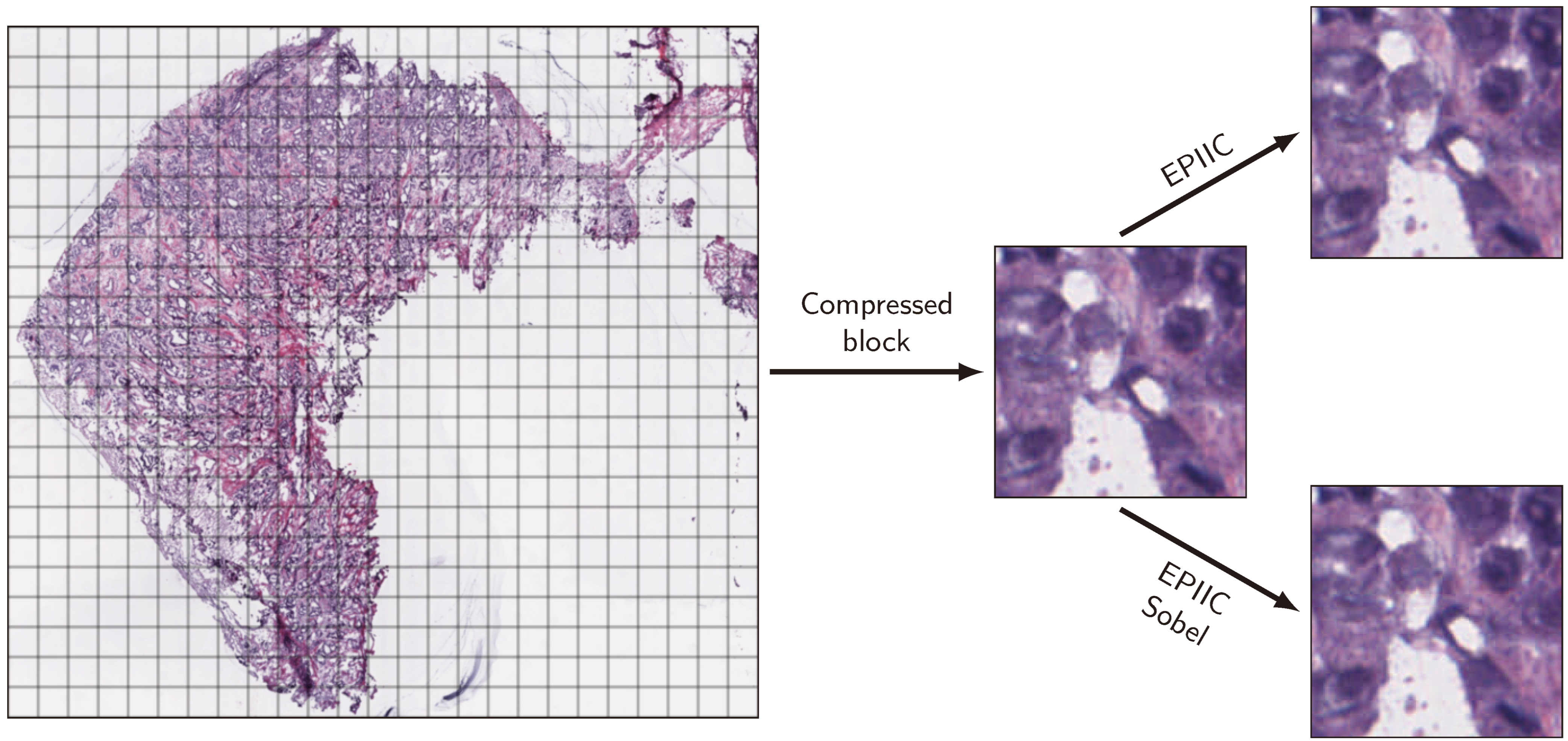
Removing compression artifacts by the EPIIC and EPIIC Sobel methods is divided into six main steps. A flowchart containing these successive steps and exemplary image fragments showing the results are shown in Figure 1.

The first step, common for both methods, involves the color deconvolution for hematoxylin-eosin staining. The algorithm explained in [24] was applied to construct an H channel image containing mostly nuclei stained by hematoxylin from eosin-stained tissue structures. A common Matlab implementation released for public use [25] was used. For other images than H&E-stained slides, the H channel image is replaced by converting the RGB image to grayscale.

The next step aims to preprocess the H image to increase the visibility of cell nuclei and reduce the noise present in the image caused by compression artifacts and the deconvolution process itself. In the EPIIC method, the threshold value is calculated first with the Otsu algorithm. Next, the contrast of the H image is adjusted by scaling the pixels with values from zero to the threshold value so that they occupy the entire allowed range of intensity values. As a result, only the most intensely colored elements are visible, and unnecessary background is removed. Then, the image is smoothed with the averaging filter to obtain more uniform shapes and colors of cell nuclei, which enables easier detection of the edges. In the EPIIC Sobel method, the image closing operation is performed on the H image with the structural element in the shape of a disk with a 3-pixel radius. After that, the contrast of an image is adjusted as before, but this time, the threshold value is fixed at 0.75. Next, the obtained image is smoothed with the averaging filter. The different threshold values make the EPIIC method better suited to images with more hematoxylin-stained structures, but in some cases, this results in the loss of poorly stained nuclei, which occurs less frequently in EPIIC Sobel.

In the next step, the gradient magnitude is calculated. In the EPIIC algorithm, the central difference method is used to calculate the gradient magnitude, which is blurred using the average smoothing filter. In the EPIIC Sobel, the gradient is calculated using the Sobel operator. The resulting image G is used to create an edge map.

In the following stage, the image G is processed to obtain the binary edge map $M_{bin}$. In the EPIIC method, the image is binarized with the Otsu method. The threshold value T obtained by the Otsu algorithm is multiplied by the $T_m$ parameter. This will ensure that weaker edges are not included in the map. This operation is followed by a morphological opening with a square-shaped structural element of size $2\times 2$ to remove isolated pixels from the map. In the EPIIC Sobel algorithm, the threshold value T is calculated based on the Root Mean Square (RMS) estimate of noise (the method described in [26], pp. 466–469), and its original value is multiplied by the $T_m$ parameter. The additional thinning stage is performed, and the opening operation is skipped. As a result of this method, the edges are much thinner than for EPIIC.

Since we are also interested in preserving information about the intensity of the edges, in the EPIIC method, the binary map $M_{bin}$ is multiplied by the image G and the pixel values are then scaled. Pixels larger than zero are reduced by the threshold value and then divided by $1-T$. Finally, the inverse image is used to obtain an edge map M. In the EPIIC Sobel variant, edge maps are created for each of the three RGB color channels. The gradient magnitudes of each channel, calculated with the central difference operator, are used instead of the image G in the multiplication. Pixel scaling is performed as in the EPIIC method. The threshold T is set to the original threshold value calculated in the previous step. To obtain the final edge maps, scaled images for each channel are inverted. Compared to the EPIIC method, which uses only the H channel to create the map, Sobel’s EPIIC method creates a separate edge map for each channel of the RGB color space.

The final step of both algorithms is weighted smoothing. First, weights for each pixel are calculated. In the EPIIC, only one weight matrix W is created by blurring the edge map M with a Gaussian filter. Then, each color channel of the compressed image is multiplied by the edge map, and the result of this operation is filtered with the same Gaussian filter used in the previous step. Pixel values are divided by corresponding weights from the W to obtain the final image $I^{\prime }$ without compression artifacts. In the EPIIC Sobel, the weight matrix is calculated for each color channel. Then, the same operations as above are performed using the edge maps and the weight matrices appropriate for the color channel.

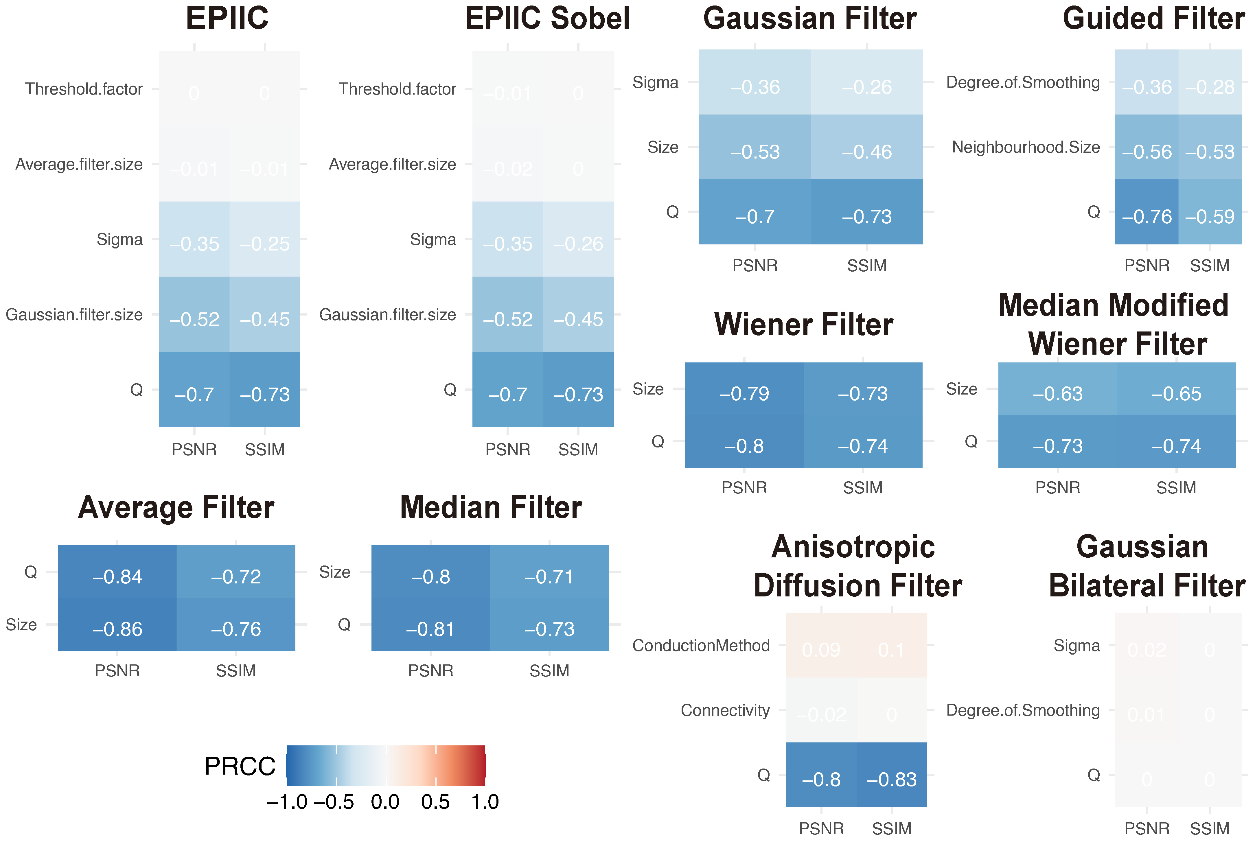
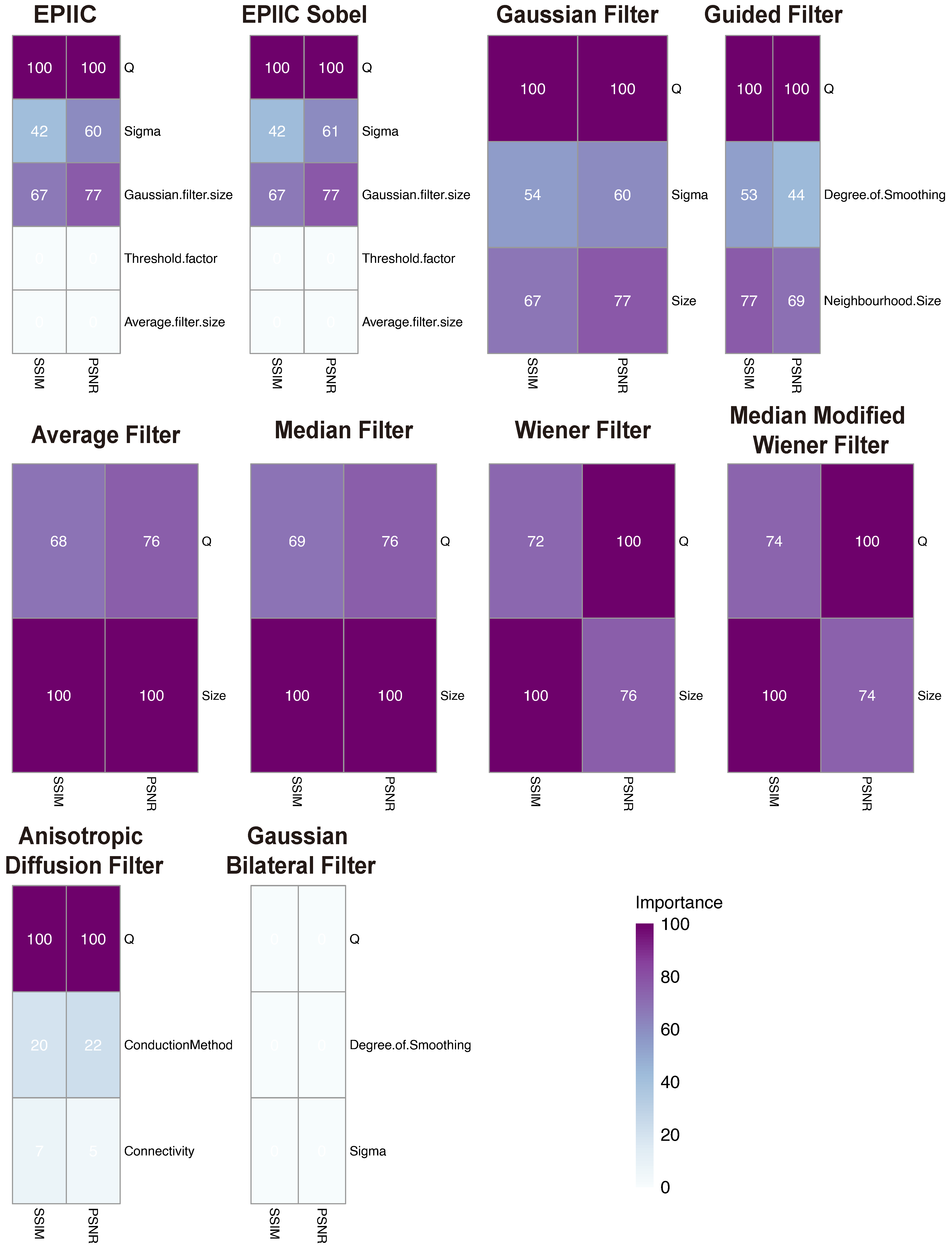
We tested both the averaging filter and the Gaussian filter with sizes ranging from $3\times 3$ to $7\times 7$. The standard deviation of the Gaussian filter varied between $0.4$ and $2.8$. Additionally, we examined the performance of different $T_m$ parameter values, which ranged from $1.25$ to $2.0$.

2.2. Other Edge-Preserving Methods

Having a strong interest in the best possible nuclei edge retention, the results of the developed methods were compared with the performance of dedicated filters for edge preservation and noise reduction.

The following filters were considered: the average (mean) filter, the median filter, the Wiener filter, which derives from the mean operator, and the Median Modified Wiener filter (MMWF), which is a nonlinear adaptive spatial filter that uses the quality and abilities of both median and Wiener filters [27]. MMWF provides global denoising, eliminating spikes and Gaussian noise while preserving the structures visible in the image. For each of the filters listed, the only parameter is the window size, which was tested in the range from 3 to 7, depending on the type of filter.

In addition, the performance of a Gaussian filter of size 3, 5, and 7 with standard deviation $\sigma$ varying from 0.4 to 2.8, and the Guided filter [28] was tested. The input image was used as a guidance image with the size of the rectangular neighborhood around each pixel from 3 to 7 and the amount of smoothing ranged from 0.001 to 0.05 (when the value is small, only the neighborhood with a small variance will be smoothed and the areas with stronger edges will be preserved).

In [29], the authors proposed a class of algorithms that realizes image denoising using a diffusion process. An anisotropic diffusion filter was used as a speckle removal technique to improve the quality of ultrasonography [30] and the magnetic resonance images [31]. In this work, different connectivity values were examined: four or eight neighborhoods and conduction methods: exponential and quadratic. In the diffusion process, five iterations were used.

In [32], the authors introduced a non-iterative bilateral filter to preserve edges through a nonlinear combination of nearby pixels. Noise removal is achieved by combining two Gaussian filters: the first works in the spatial domain, and the second filter works in the intensity domain. This filter applies spatially weighted averaging to smooth edges and preserve their shape. This method was also used to eliminate distortions from medical images [30]. Here, degrees of smoothing from 0.005 to 0.02 and standard deviations of spatial Gaussian smoothing kernel from 0.4 to 1.3 were tested.

Another tested algorithm, the non-local means (NL-means), based on a non-local averaging of all pixels in the image, was presented in [33]. It can smooth blocking artifacts and preserve the edges simultaneously. Due to the nature of the algorithm, the most favorable case is the textured or periodic image, but some natural images also have sufficient redundancy for the filtering action to have a positive impact on image quality.

Finally, the deep convolutional neural network FBCNN [20], which achieves state-of-the-art performance in the blind JPEG artifacts removal on single and multiple compressed color and grayscale images, was tested. Trained weights were used for a model designed to remove single compression artifacts from color images provided by the authors (https://github.com/jiaxi-jiang/FBCNN/releases/tag/v1.0, accessed on 4 February 2025).

2.3. Compression Artifacts Removal Evaluation

Two common metrics to evaluate the quality of reconstructed images after compression artifacts removal were calculated: Peak Signal-to-Noise Ratio ($PSNR$) and Structural Similarity Index Measure ($SSIM$) [34]. $PSNR$ can be represented as follows:

$$\begin{array}{c}\hfill PSNR=10·lo{g}_{10}\left({\displaystyle \frac{MA{X}_I^2}{MSE}}\right)\end{array}$$

(1)

where $MA{X}_I^2$ is the maximum possible pixel value for the given range, and the Mean Squared Error ($MSE$) is calculated by averaging the squared intensity differences between two images. $SSIM$ for given original image I and transformed image J is defined by the following formula:

$$\begin{array}{c}\hfill SSIM={\displaystyle \frac{(2{\mu }_I{\mu }_J+C_1)(2{\sigma }_{IJ}+C_2)}{({{\mu }_I}^2+{{\mu }_I}^2+C_1)({{\sigma }_J}^2+{{\sigma }_J}^2+C_2)}}\end{array}$$

(2)

where $\mu$ is the average and $\sigma$ is the variance of pixel intensity. $SSIM$ is generally regarded as a closer metric to human perception than $PSNR$.

2.4. Sensitivity Analysis

To determine how changing the parameters of compression artifacts removal methods affects the final image quality, two methods were implemented. The difference in $SSIM$ and $PSNR$ between the analyzed method and compressed images were used as image quality metrics. First, the Partial Rank Correlation Coefficient (PRCC), which measures nonlinear and monotonic relationships between parameters and image quality metrics, was calculated. PRCC uses the Spearman correlation after removing linear dependencies between parameters. Second, the impact of parameters on image quality was estimated using the variable importance measure from the multivariate adaptive regression spline (MARS) model implemented in the caret R package [35]. Specifically, the changes in the generalized cross-validation estimate of error for each predictor are tracked, and reductions in the statistic when each predictor’s feature is added to the model are accumulated. The variable importance is scaled to sum up to 100%.

2.5. Nuclei Segmentation Methods

Two state-of-the-art nuclei instance segmentation methods, Hover-Net [36] and STARDIST [37], were employed to assess the impact of developed methods on the segmentation quality.

The Hover-Net network received an input RGB patch of $270\times 270$, with values normalized between 0 and 1. Since we wanted to verify whether removing compression artifacts would cause segmentation improvement, reference models were trained for each dataset separately using original images without any modification for training and validation. These models were marked as no correction method. For reference models, in online augmentation, identical techniques were used as in the original paper [36], that is, flip, rotation, Gaussian blur, median blur, additive Gaussian noise, modification of contrast, hue, and saturation.

Next, we trained models for each selected artifact removal method for each dataset. First, compression artifacts were removed from images from the training and test sets. The EPIIC and EPIIC Sobel methods used a Gaussian filter with a window size of $3\times 3$ and a standard deviation $\sigma =0.7$, a parameter $T_m=1.25$, and an averaging filter of size $5\times 5$. For the Gaussian filtering, the same $\sigma$ and kernel size were used as in the previous methods. For the Guided filter, we set the degree of smoothing to $0.001$ and the neighborhood size to 3. During model training, the augmentation was limited to flip, rotation, contrast modification, hue, and saturation.

All models described above were initialized with pre-trained weights on the ImageNet dataset [38]. Only decoders were trained for the first 50 epochs, and then all layers were fine-tuned for 75 epochs. The Adam optimizer was used with the following learning schedule: for each stage, the initial value of the learning rate was ${10}^{-4}$, and after every 25 epochs, it was reduced ten times. Batch size was set to 10 and 2 for the first and second stages, respectively. An early stopping method with patience equal to 50 was used by selecting the model that achieved the best $DICE$ score on the validation dataset.

The STARDIST model with 64 rays and a U-Net [39] backbone of depth 4 was used. The dropout equal to 0.7 was added to the network to avoid overfitting, and loss functions specified by the authors were used. The weights of the network were initialized randomly. Each model was trained for 400 epochs with a batch size equal to 2 using the Adam optimizer, starting with a learning rate of 0.0003. If no progress was made for 80 epochs, the learning rate was reduced by half. The weights for the final model were selected based on the smallest validation loss during training. The network received an RGB input patch with a size of $256\times 256$ normalized to the range 0–1. The same online augmentation procedure as for the Hover-Net model was applied.

2.6. Nuclear Segmentation Evaluation Metrics

To evaluate the overall score for nuclear instance segmentation, three metrics widely used in the literature were used: Ensemble Dice [40], Aggregated Jaccard Index ($AJI$) [41], and Panoptic Quality ($PQ$) [42]. Ensemble Dice computes and aggregates Dice coefficient ($DICE$) per nucleus, which is defined as:

$$\begin{array}{c}DICE=2\times {\displaystyle \frac{X\cap Y}{\left|X\right|+\left|Y\right|}}\end{array}$$

(3)

where X denotes the ground truth and Y is a prediction. It is usually used to calculate the similarity of two samples. $AJI$ calculates the ratio of an aggregated intersection cardinality and an aggregated union cardinality between the ground truth and the prediction. $PQ$ for nuclear segmentation is defined as the product of the Detection Quality ($DQ$) and the Segmentation Quality ($SQ$):

$$\begin{array}{c}PQ=DQ\times SQ\end{array}$$

(4)

The Detection Quality ($DQ$) can be interpreted as the F1-score, which is widely used to evaluate instance detection. At the same time, segmentation quality ($SQ$) informs how close each correctly detected instance is to its matched ground truth. The following formulas describe these measures:

$$\begin{array}{c}DQ={\displaystyle \frac{\left|TP\right|}{\left|TP\right|+\frac{1}{2}\left|FP\right|+\frac{1}{2}\left|FN\right|}}\end{array}$$

(5)

$$\begin{array}{c}SQ={\displaystyle \frac{{\sum }_{(x,y)\in TP}IoU(x,y)}{\left|TP\right|}}\end{array}$$

(6)

where x stands for a ground truth segment, y is a prediction segment and $IoU$ denotes intersection over union. $PQ$ provides a direct insight into the detection quality of individual nuclear instances and the segmentation of each detected nucleus. If the $IoU(x,y)>0.5$ each $(x,y)$ pair is unique [42]. This property allows to divide the predicted and ground truth segments into the following sets: true positives (TP), false positives (FP), and false negatives (FN), which represent correctly matched pairs of segments, mismatched predicted segments, and mismatched ground truth segments, respectively.

2.7. Datasets

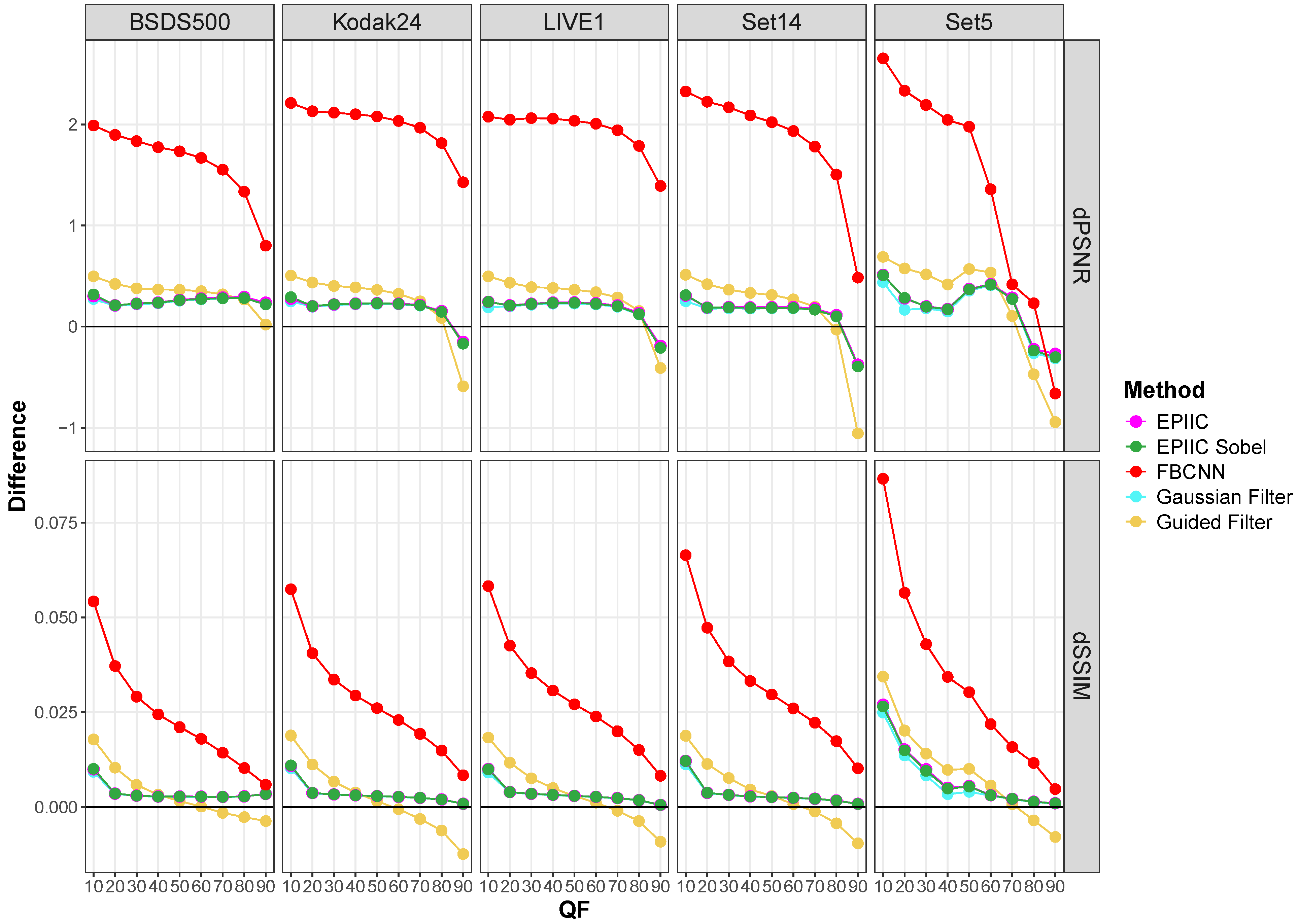
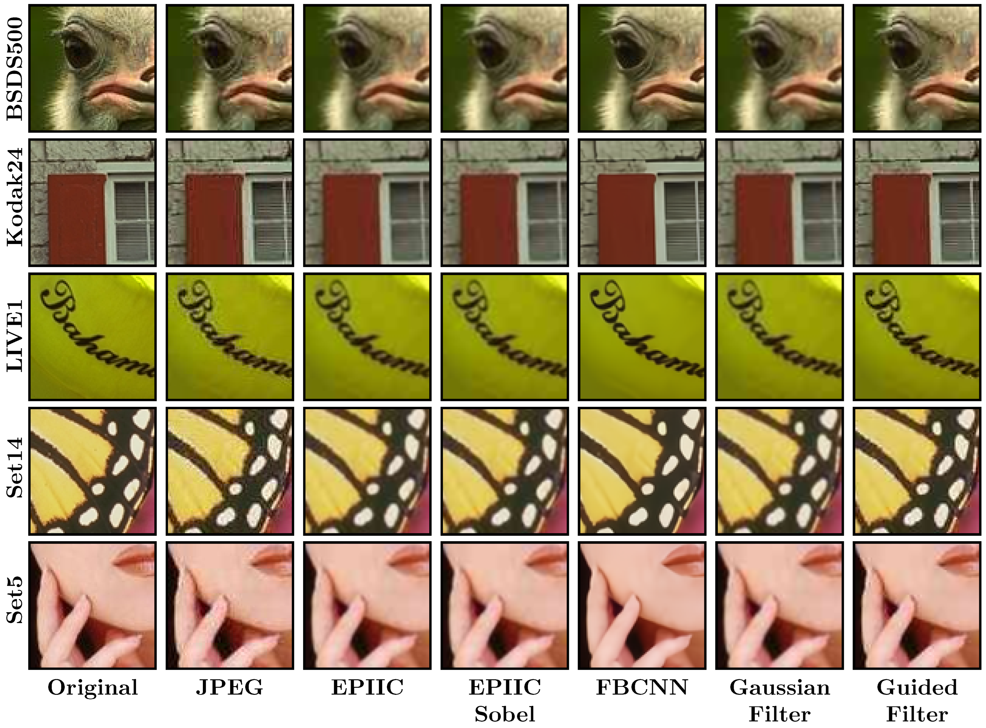
Several datasets were used to evaluate the impact of selected artifacts removal methods on the image quality. The BreCaHAD dataset [43] includes 162 uncompressed histopathological RGB images showing tissue sections with breast cancer cells. The images are divided into 17 different cases. Each image was taken with 40× magnification and then divided into smaller tiles saved as $1360\times 1024$ TIFF files. The proposed methods were also tested on the datasets commonly used in a task of compression artifacts removal: the test set of BSDS500 [44], LIVE1 [45], Kodak24 (https://r0k.us/graphics/kodak/, accessed on 4 February 2025) Set5 [46], and Set14 [47]. All of these datasets consist of uncompressed RGB images.

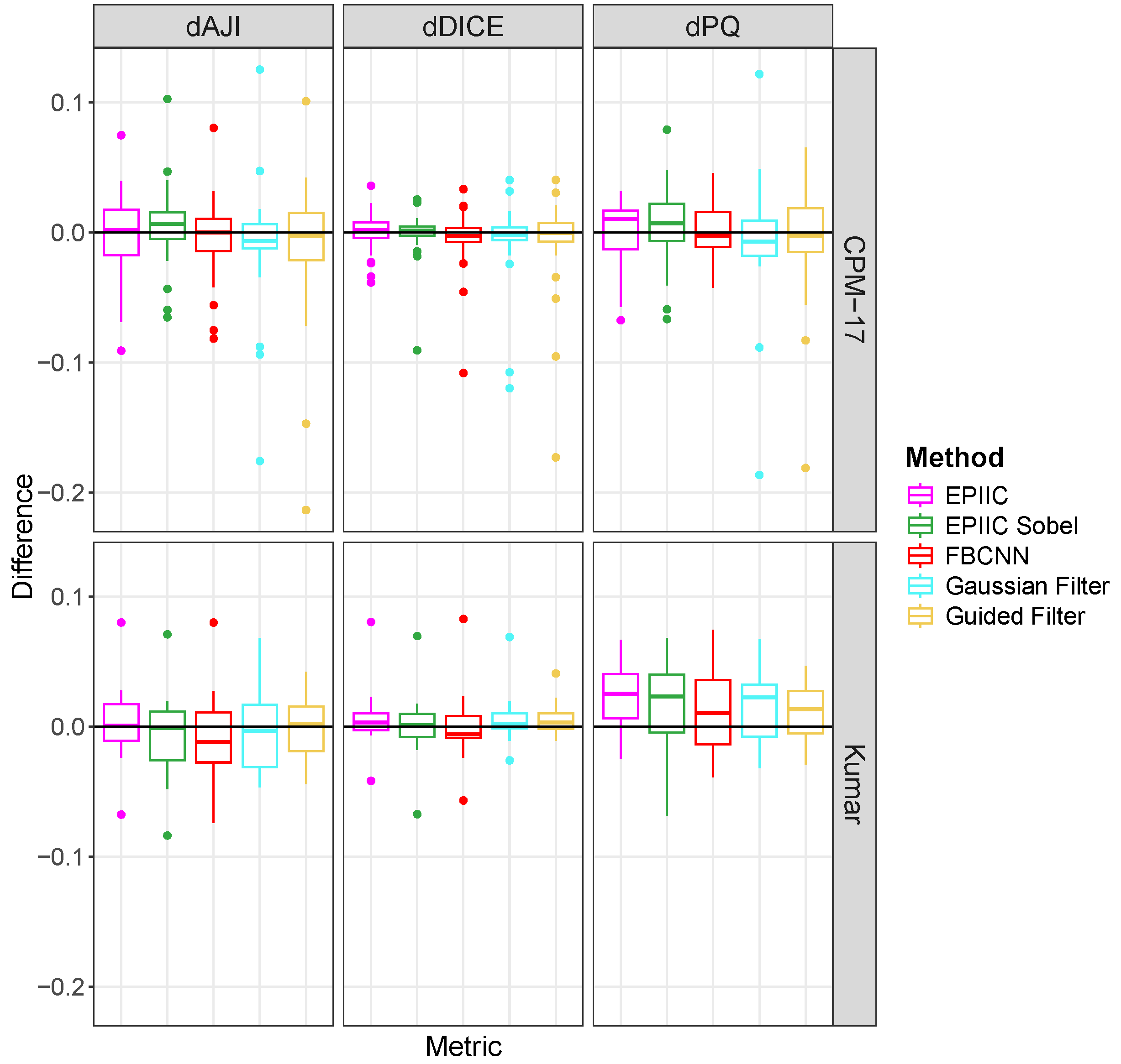
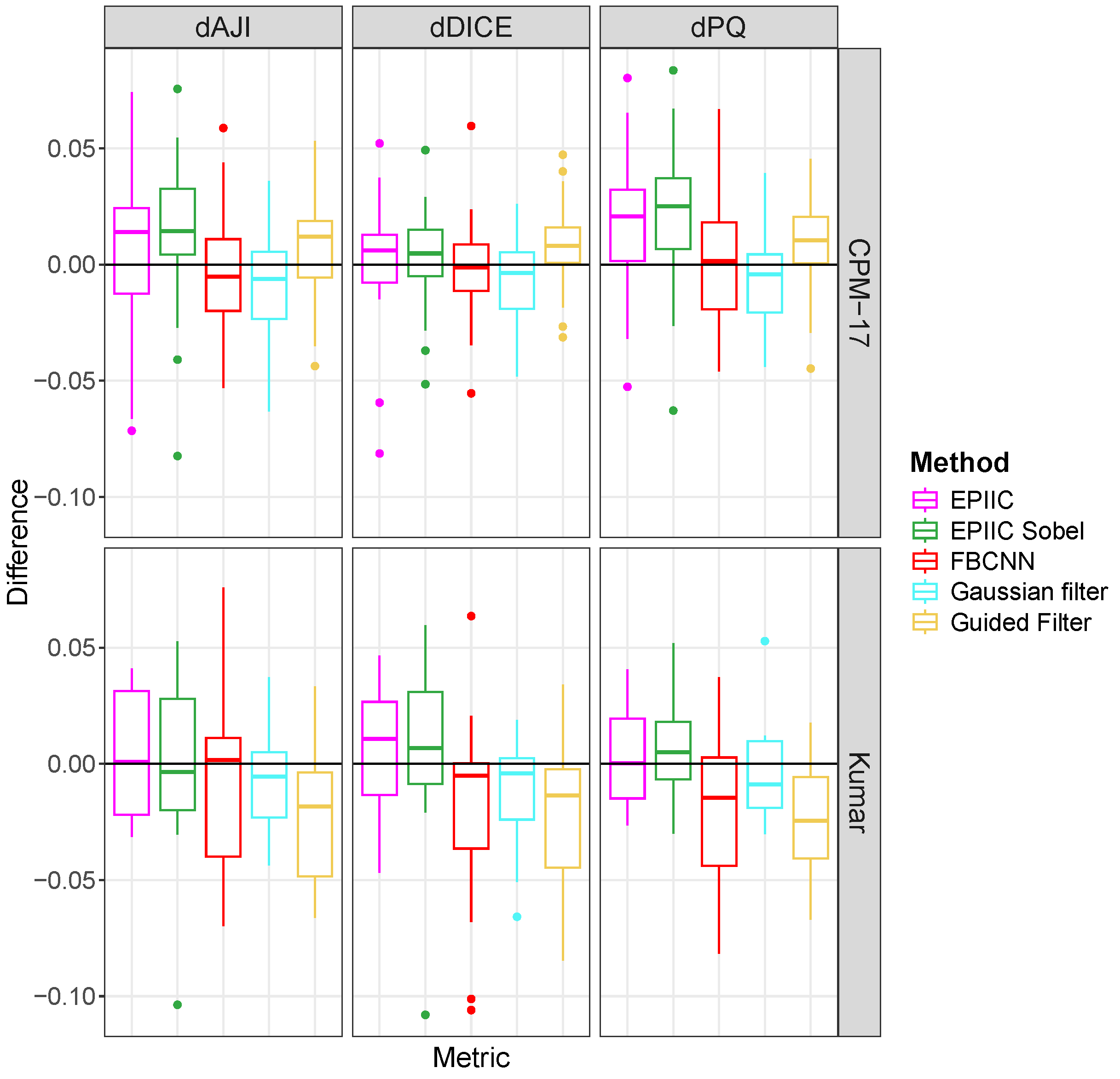
Since the BreCaHAD dataset is not labeled for the nuclear segmentation task, two additional datasets were used: Kumar [41] and CPM-17 [40]. Both datasets contain compressed images of varying quality, with visible JPEG compression artifacts, but the information about the compression quality factor is not included. The Kumar dataset consists of 30 image tiles of size $1000\times 1000$. Slides were acquired at $40\times$ magnification and come from seven organs (6 breasts, 6 livers, 6 kidneys, 6 prostates, 2 bladders, 2 colons, and 2 stomachs) of The Cancer Genome Atlas (TCGA) database. We split this dataset into the test set with 14 images (2 prostates, 2 kidneys, 2 livers, 2 breasts, 2 bladders, 2 colons, and 2 stomachs) and the training set with 16 image tiles (4 prostates, 4 kidneys, 4 livers, and 4 breasts). The CPM-17 dataset includes 32 images from TCGA varying in size from $500\times 500$ to $600\times 600$ in both the training and test datasets. Images were taken at $20\times$ and $40\times$ magnification and included four different types of cancer. Note, we utilize the same split used in the [36] for both datasets.

2.8. Whole-Slide Images Processing

The developed algorithms have been implemented to process entire WSI images in the Matlab R2022b software. Figure 2 illustrates the process of removing artifacts. The code is publicly available in a remote repository https://github.com/julimer228/EPIIC, accessed on 4 February 2025). The image with the coarsest resolution is divided into blocks. Each block is then processed separately using the selected method. Appropriate padding with a default value of 5 pixels is set to prevent distortion of block edges. In the next step, the image is scaled to successive layers of lower resolution according to the information read from the original image. Layers that are included as labels are rewritten in the original order. After removing the artifacts, the image is compressed using the lossless LZW compression algorithm [48], which does not decrease image quality but reduces the size of the resulting file. The example WSI image of 299 MB after artifacts removal increased its size to 2.69 GB for both methods.

3. Results

3.1. Improving Image Quality by Removing Compression Artifacts

In all analyses, we compressed the original images with JPEG compression quality factor $QF$ values from 10 to 90 in increments of 10. We then tested each described method for removing compression artifacts in terms of the quality of reconstructed images and compared them to results obtained for JPEG compressed images.

The results for histopathological H&E stained images are presented in

Table 1. $SSIM$ and $PSNR$ scores for the BreCaHAD dataset. The first, the second, and the third best results are highlighted.

Method	Metric	QF = 10	QF = 20	QF = 30	QF = 40	QF = 50	QF = 60	QF = 70	QF = 80	QF = 90
JPEG	$SSIM$	0.8259	0.8928	0.9195	0.9330	0.9422	0.9495	0.9571	0.9646	0.9728
	$PSNR$	29.76	33.05	34.82	35.98	36.86	37.67	38.65	39.83	41.41
EPIIC	$SSIM$	0.8790	0.9213	0.9391	0.9483	0.9545	0.9595	0.9649	0.9701	0.9757
	$PSNR$	30.93	34.07	35.75	36.85	37.67	38.42	39.31	40.33	41.56
EPIIC Sobel	$SSIM$	0.8790	0.9213	0.9390	0.9483	0.9545	0.9595	0.9649	0.9701	0.9757
	$PSNR$	30.93	34.08	35.76	36.86	37.67	38.43	39.32	40.34	41.58
FBCNN	$SSIM$	0.9029	0.9403	0.9546	0.9617	0.9664	0.9701	0.9739	0.9774	0.9814
	$PSNR$	32.52	35.44	36.94	37.86	38.55	39.13	39.84	40.64	41.67
Gaussian Filter	$SSIM$	0.8786	0.9211	0.9390	0.9482	0.9544	0.9594	0.9648	0.9701	0.9756
	$PSNR$	30.91	34.05	35.74	36.83	37.66	38.41	39.30	40.31	41.54
Guided Filter	$SSIM$	0.8784	0.9217	0.9384	0.9476	0.9536	0.9582	0.9628	0.9672	0.9715
	$PSNR$	30.94	34.12	35.77	36.85	37.68	38.39	39.22	40.13	41.18
Average Filter	$SSIM$	0.8751	0.9205	0.9388	0.9477	0.9535	0.9579	0.9624	0.9667	0.9709
	$PSNR$	30.82	34.04	35.72	36.76	37.51	38.16	38.89	39.68	40.54
Median Filter	$SSIM$	0.8611	0.9115	0.9328	0.9431	0.9499	0.9551	0.9604	0.9656	0.9709
	$PSNR$	30.57	33.70	35.42	36.52	37.32	38.02	38.84	39.76	40.85
Wiener Filter	$SSIM$	0.8754	0.9193	0.9386	0.9479	0.9538	0.9585	0.9630	0.9674	0.9718
	$PSNR$	30.86	33.98	35.73	36.83	37.63	38.33	39.13	40.00	40.99
Non-local Means Filter	$SSIM$	0.8259	0.8928	0.9195	0.9330	0.9422	0.9495	0.9571	0.9646	0.9729
	$PSNR$	29.76	33.05	34.82	35.98	36.86	37.67	38.65	39.83	41.41
Median Modified Wiener Filter	$SSIM$	0.8596	0.9095	0.9322	0.9431	0.9501	0.9556	0.961	0.9663	0.9718
	$PSNR$	30.52	33.73	35.40	36.54	37.38	38.13	39.01	40.01	41.21
Anisotropic Diffusion Filter	$SSIM$	0.8750	0.9216	0.9385	0.9466	0.9518	0.9558	0.9597	0.9635	0.9672
	$PSNR$	30.83	34.10	35.71	36.70	37.40	37.98	38.64	39.33	40.05
Gaussian Bilateral Filter	$SSIM$	0.8259	0.8928	0.9195	0.9330	0.9422	0.9495	0.9571	0.9646	0.9728
	$PSNR$	29.76	33.05	34.82	35.98	36.86	37.67	38.65	39.83	41.41

. We included the best mean $SSIM$ and $PSNR$ scores obtained by each method for the tested parameter sets. Figure 3 depicts fragments of uncompressed histopathological images, images after compression, and the effects of removing compression artifacts by methods that obtained the highest image quality: EPIIC, EPIIC Sobel, FBCNN, the Gaussian filter, and the Guided filter. As can be seen, the deep learning-based solution significantly outperformed the other methods. However, our proposed artifact removal methods improved image quality for all tested compression quality parameters. They were also slightly better than the Gaussian filter in most cases. The EPIIC method performed worse than the Sobel variant. The Guided filter gave more satisfying results for images compressed with lower $QF$ values than the mentioned filtering methods. If we carefully look at the images processed by the network, we can see some smoothing and unification of the color of the structures visible in the image. The images processed by the developed methods are blurred. However, they allowed slightly better preservation of the minor color variations in the actual tissue image.

The best methods mentioned above were evaluated on other image datasets containing natural images. Again, the best results for most cases were achieved by the FBCNN neural network. The EPIIC, EPIIC Sobel, Gaussian Filter, and Guided filter algorithms also improved the average $SSIM$ and $PSNR$ scores for selected datasets for most of the tested $QF$ values. The best results of each method are included in the Appendix A. The diagram presented in Figure 4 shows the average difference between the $SSIM$ and $PSNR$ values before and after removal of the blocking artifacts for the top four methods. Some examples of the outcomes are presented in Figure 5.

The comparison of computational time presented in

Table 2. Comparison of computing times for the tested methods on the BreCaHAD dataset. The reported values include the mean, standard deviation, and median time in seconds.

Method	Mean [s]	Std [s]	Median [s]
EPIIC	0.187	0.046	0.178
EPIIC Sobel	0.316	0.053	0.308
FBCNN (CPU)	17.052	0.642	16.980
FBCNN (GPU)	1.043	0.050	1.039
Gaussian Filter	0.011	0.003	0.011
Guided Filter	0.223	0.038	0.223
Average Filter	0.010	0.003	0.010
Median Filter	0.053	0.009	0.053
Wiener Filter	0.085	0.016	0.083
Non-local Means Filter	2.490	0.238	2.461
Median Modified Wiener Filter	2.060	0.139	2.054
Anisotropic Diffusion Filter	12.082	9.217	9.686
Gaussian Bilateral Filter	0.472	0.062	0.470

shows the average, standard deviation, and median time per image calculated on the BreCaHAD dataset. The tests were conducted on a workstation equipped with a 12th Gen Intel Core i9-12900KF processor (16 cores, 24 threads, 800–5200 MHz; Intel Corporation, Santa Clara, CA, USA) and an NVIDIA GeForce RTX 3060 GPU (NVIDIA Corporation, Santa Clara, CA, USA). It can be concluded that the developed methods are slightly slower compared to classical filters, such as the Gaussian and average filters. Additionally, the Sobel variant is slower than the EPIIC method. However, they perform significantly faster than the FBCNN method, even when a graphics card is used for the inference, which makes the proposed methods better suited for processing large WSI images.

For each artifacts removal method, we estimated which parameters have the highest impact on image quality by calculating two metrics: PRCC (Figure A1) and variable importance (Figure A2). Additionally, we included the Quality Factor ($QF$) in the analysis to show if the achieved gain in image quality compared to JPEG compressed images varies with the compression ratio. In all methods, $QF$ was negatively correlated with gain in $PSNR$ and $SSIM$, meaning a higher need for artifacts removal for low $QF$ values. Also, the highest variable importance value for this factor was observed in most cases. For EPIIC and EPIIC Sobel, window size and the standard deviation of the Gaussian filter have a higher influence on the results than the two other parameters. Similarly, in the other methods, changing window size resulted in different image quality, so it is an important parameter to tune. For the Anisotropic Diffusion Filter, we observe a small influence of changing parameters on the results, while for the Gaussian Bilateral Filter, no influence was observed for the tested parameter ranges.

3.2. Impact of Compression Artifacts Removal on Nuclei Segmentation

The main purpose of removing compression artifacts from HE-stained images is to improve the performance of further analysis, e.g., segmentation of cell nuclei. We tested the performance of the nuclei segmentation using Hover-Net and STARDIST models after the application of the four best artifact removal methods. Two datasets were used in this analysis: Kumar and CPM-17.

We calculated the difference between the performance scores obtained for each image processed without removing compression artifacts (marked as no correction) and images after removal.

Table 3. The table presents the performance of competing methods on the Kumar and CPM-17 datasets for both segmentation methods. The best results are underlined.

Dataset	Segmentation Method	Method	Mean			Median
			$\Delta$$\mathbf{DICE}$	$\Delta$$\mathbf{AJI}$	$\Delta$$\mathbf{PQ}$	$\Delta$$\mathbf{DICE}$	$\Delta$$\mathbf{AJI}$	$\Delta$$\mathbf{PQ}$
CPM-17	Hover-Net	EPIIC	0.0002	−0.0030	0.0005	0.0018	0.0018	0.0105
		EPIIC Sobel	−0.0010	0.0045	0.0056	0.0013	0.0068	0.0072
		FBCNN	−0.0054	−0.0044	0.0016	−0.0029	−0.0001	−0.0024
		Gaussian Filter	−0.0052	−0.0026	−0.0026	−0.0020	0.0014	−0.0005
		Guided Filter	−0.0069	−0.0100	−0.0058	−0.0003	−0.0025	−0.0024
	STARDIST	EPIIC	0.0026	0.0087	0.0169	0.0061	0.0140	0.0207
		EPIIC Sobel	0.0038	0.0135	0.0217	0.0048	0.0144	0.0251
		FBCNN	−0.0018	−0.0045	0.0025	−0.0018	−0.0056	0.0014
		Gaussian Filter	−0.0058	−0.0083	−0.0053	−0.0036	−0.0062	−0.0043
		Guided Filter	0.0075	0.0089	0.0082	0.0080	0.0119	0.0105
Kumar	Hover-Net	EPIIC	0.0066	0.0028	0.0234	0.0034	0.0006	0.0254
		EPIIC Sobel	0.0008	−0.0073	0.0155	0.0013	−0.0011	0.0231
		FBCNN	0.0007	−0.0068	0.0124	−0.0058	−0.0119	0.0106
		Gaussian Filter	0.0036	−0.0085	0.0172	0.0000	−0.0055	0.0229
		Guided Filter	0.0063	−0.0007	0.0110	0.0034	0.0022	0.0135
	STARDIST	EPIIC	0.0068	0.0043	0.0020	0.0107	0.0009	0.0003
		EPIIC Sobel	0.0044	−0.0020	0.0060	0.0067	−0.0035	0.0050
		FBCNN	−0.0185	−0.0071	−0.0194	−0.0051	0.0016	−0.0146
		Gaussian Filter	−0.0130	−0.0078	−0.0041	−0.0041	−0.0056	−0.0088
		Guided Filter	−0.0236	−0.0217	−0.0252	−0.0136	−0.0183	−0.0244

and box plots in Figure 6 and Figure 7, contain the outcomes of selected segmentation measures for both nuclei segmentation methods. We conducted a Wilcoxon test to determine if the results were statistically significant. The p-values for each measure are shown in the

Table 4. The table presents the p-values of the Wilcoxon test.

Dataset	Segmentation Method	Method	$\mathbf{DICE}$	$\mathbf{AJI}$	$\mathbf{PQ}$
CPM-17	Hover-Net	EPIIC	$2.052\times {10}^{-1}$	$5.037\times {10}^{-1}$	$2.270\times {10}^{-1}$
		EPIIC Sobel	$1.391\times {10}^{-1}$	$8.888\times {10}^{-2}$	$6.440\times {10}^{-2}$
	STARDIST	EPIIC	$1.024\times {10}^{-1}$	$4.540\times {10}^{-2}$	$1.500\times {10}^{-3}$
		EPIIC Sobel	$9.840\times {10}^{-2}$	$4.700\times {10}^{-3}$	$8.19\times {10}^{-5}$
Kumar	Hover-Net	EPIIC	$1.206\times {10}^{-1}$	$3.349\times {10}^{-1}$	$4.300\times {10}^{-3}$
		EPIIC Sobel	$4.039\times {10}^{-1}$	$7.292\times {10}^{-1}$	$5.020\times {10}^{-2}$
	STARDIST	EPIIC	$3.910\times {10}^{-1}$	$3.910\times {10}^{-1}$	$7.609\times {10}^{-1}$
		EPIIC Sobel	$2.958\times {10}^{-1}$	$8.552\times {10}^{-1}$	$3.575\times {10}^{-1}$

. The developed methods improved the results, particularly considering the $PQ$ measure. Figure 8 presents the example segmented images for both datasets with Hover-Net models.

As can be seen for some nuclei, the EPIIC and EPIIC Sobel methods allowed more precise nuclei detection. It can also be seen that some instances that were not detected by the no-correction Hover-Net model were detected after artifacts removal. In addition, note the results of image segmentation after removing compression artifacts with the Guided filter. For the first of the presented image fragments from the CPM-17 set, a sizable section between the nuclei with irregular outlines was marked as the nucleus area. Such a phenomenon can be a significant obstacle in using this algorithm to remove compression artifacts.

Moreover, the median differences of $DICE$, $AJI$, and $PQ$ for this method do not indicate such significant differences in segmentation results. The FBCNN network allowed for enhanced image quality, but for most images, it caused the degradation of the segmentation performance for both tested segmentation models. The developed edge-preserving algorithms also achieved slightly better results than the Gaussian filter with the same parameters.

4. Discussion

The edge-preserving methods we introduced here allowed us to successfully remove compression artifacts and improve the overall image quality. We decided to take into account the color intensity values on the edges instead of simple binarization as in the original method described in [23]. Moreover, we used color stain deconvolution to extract the information about the nuclei boundaries more precisely, which allowed us to improve the image quality more than other non-deep learning methods for most compression quality factors used in the JPEG algorithm. The developed methods were designed to process H&E images but also improved the quality of compressed images from multiple other datasets with various origins (mostly natural images). The results of EPIIC and EPIIC Sobel achieved for images from datasets commonly used to show the efficiency of different compression artifacts removal algorithms and the BreCaHAD dataset are inferior to those for the method based on deep learning. This outcome was rather expected since our goal was to ensure the simplicity of the developed algorithms even at the cost of performance because they are designed to be used to process large WSI images. FBCNN on CPU was almost 100 times slower than EPIIC, while on GPU, it was still more than 5 times slower. However, a comparison of all deep learning-based methods and our methods in terms of computational efficiency on WSI images is needed.

The main drawback of compression of WSI images is the reduced efficiency of algorithms used to segment individual cells or important fragments of the tissue. We introduced edge-preserving methods that could efficiently remove blocking artifacts but that should not decrease the performance of cell/tissue segmentation methods. Note that the developed methods are based on classical image processing operations. Unlike deep neural networks, they do not require datasets to train the model. The developed methods improved performance and allowed more accurate detection of nuclear instances.

$DICE$ and $AJI$ have a limitation: predictions that differ by only a few pixels can have significantly different $AJI$ and $DICE$ results, particularly when two nuclei are adjacent and only one is detected. This can strongly affect the accurate evaluation of segmentation results, especially if the tissue image contains a lot of difficult-to-detect instances. Therefore, using the $PQ$ measure to assess the segmentation quality allows for a more reliable analysis of the results. Based on $PQ$, EPIIC and EPIIC Sobel led to better nuclei segmentation results than all other methods.

Interestingly, processing the images with FBCNN, which performed best in removing artifacts in most cases, caused a decline in segmentation results tested by two different models. It is worth noting that this particular method takes the $QF$ parameter value into account when eliminating distortions. The FBCNN method focuses on improving image quality, and the methods we propose are aimed at improving segmentation quality. Using the generated edge maps, the pixels along cell edges undergo less blurring compared to those inside the cells, resulting in better preservation of these regions. The proposed edge-preserving algorithms provided better results than Gaussian blur in terms of both segmentation results and image quality improvement. The Guided filter enabled improved image quality, especially for small $QF$ values. However, the incorrect predictions seen in some of the segmentation results bring into doubt the validity of applying this method to the removal of blocking artifacts from histopathology images.

Both datasets contained compressed images with different values of the $QF$ parameter, and nuclei determinations were already made on the compressed images, which could have affected the results. To better evaluate the methods mentioned above, testing their performance on datasets labeled before compression would be necessary. Further testing is required on other datasets from different sources containing preparations from other tissue types. It is necessary to keep working on fine-tuning the algorithm’s parameters to the degree of image compression. In future analyses, it would also be worth checking the performance of edge-preserving filters based on deep-learning methods and hybrid solutions that combine classical techniques with deep-learning approaches. Such solutions have already been applied to remove additive white Gaussian noise from biomedical images [49].

An additional advantage of our methods is the ability to remove JPEG compression artifacts from entire WSI images. When artifacts are removed, the size of the image increases, which is obvious. However, it should be considered whether that is a significant disadvantage if this process can result in enhanced segmentation results.

5. Conclusions

We developed two edge-preserving methods for removing compression artifacts in histopathological images. The developed methods were efficient even for images compressed with a low compression quality factor. Despite this, tests conducted on both HE-stained images and popular image datasets indicated worse performance than the tested deep learning method; our methods improved segmentation for the two selected datasets compared to the state-of-the-art neural network. Since the proposed solutions are faster than DL-based methods, we adopted the algorithms to process the entire gigapixel WSI.