HG-LGBM: A Hybrid Model for Microbiome-Disease Prediction Based on Heterogeneous Networks and Gradient Boosting

Abstract

The microbiome plays a crucial role in maintaining physiological homeostasis and is intricately linked to various diseases. Traditional culture-based microbiological experiments are expensive and time-consuming. Therefore, it is essential to prioritize the development of computational methods that enable further experimental validation of disease-associated microorganisms. Existing computational methods often struggle to effectively capture nonlinear interactions and heterogeneous network structures when predicting microbiome–disease associations. To address this issue, we propose HG-LGBM, an innovative joint prediction framework that combines heterogeneous graph neural networks with a gradient boosting mechanism. We employ a hierarchical heterogeneous graph transformer (HGT) encoder, which utilizes a multi-head attention mechanism to learn higher-order node representations, while LightGBM optimizes the classification task using gradient-boosted decision trees. Evaluated through five-fold cross-validation on the HMDAD and Disbiome datasets, HG-LGBM demonstrated a state-of-the-art performance. The experimental results showed that combining heterogeneous network learning with gradient boosting strategies effectively revealed potential microbiome–disease interactions, providing a powerful tool for biomedical research and precision medicine. Finally, case studies on colorectal cancer and inflammatory bowel disease (IBD) further validated the effectiveness of HG-LGBM.

1. Introduction

The human microbiome consists of dynamic microbial communities that inhabit various anatomical locations in the body, such as the gut, mouth, and skin. These communities form stable symbiotic relationships with the host [1,2,3]. The microbiome exhibits distinct functional characteristics influenced by environmental and host factors throughout different life stages. It plays a crucial role in maintaining bodily balance and immune function, but disruptions in the microbiome can lead to the dysregulation of body functions and different metabolic disturbances, which may trigger various diseases [4], including cardiovascular disease (CVD) [5], cancer [6], metabolic diseases [7], and inflammatory bowel disease (IBD) [8]. With advances in microbiome-targeted therapeutic strategies, microbial-based treatments such as fecal microbiota transplantation (FMT) [9,10] and probiotics/prebiotics regulation [11] have shown significant success in the prevention and treatment of diseases like inflammatory bowel disease [12] and Alzheimer’s disease [13]. These approaches are gradually expanding to areas such as diabetes [14] and Parkinson’s disease [15]. Therefore, integrating multi-source biomedical data to further explore the potential connections between microbiomes and diseases is crucial for understanding disease mechanisms and advancing precise microbiome-based treatments [16].

Depending on the prediction strategy, the current computational methods for predicting microbiome–disease associations include network propagation-based approaches, matrix factorization techniques, random walk algorithms, and machine learning and deep learning models [17]. Network-based methods construct a relationship network between microorganisms and diseases, using network analysis techniques to reveal potential associations. KATZHMDA [18], a pioneering framework for network topology analysis, quantifies cross-species associations by defining the KATZ similarity score between microorganisms and disease nodes in a heterogeneous network. PBHMDA [19] introduces a depth-first search strategy into heterogeneous networks to infer relationships between microorganisms and diseases. MATHNMDA [20] uses a graph neural network based on heterogeneous networks and meta-path aggregation to predict associations between microorganisms and diseases. Random walk methods simulate the propagation of data points within a network, using paths in the graph to infer potential associations between microorganisms and diseases. The BiRWHMDA [21] model employs a bidirectional random walk algorithm to construct a probability transition matrix within a similarity network between microorganisms and diseases, predicting potential microbiome–disease associations. Matrix factorization methods decompose microbiome–disease association data (typically sparse matrices) into low-dimensional representations, revealing potential associations. The GRNMFHMDA [22] model uses graph regularization constraints on the objective function to capture linear relationships in the data. MNNMDA [23] applies the Matrix Nuclear Norm method to known microbiome and disease data to predict microbiome–disease associations. Machine learning and deep learning models learn patterns from data through training algorithms to predict associations between microorganisms and diseases [24]. The SAELGMDA [25] model uses a graph learning method based on autoencoders and enhances the representation learning ability of traditional graph autoencoders by incorporating a self-attention mechanism. It classifies microbiome–disease pairs using LightGBM. GATMDA [26] employs a Graph Attention Network (GAT) to model microorganism and disease nodes to enable the capture of complex interactions between the nodes by weighting the information from their neighboring nodes using an attention mechanism. DAEGCNDF [27] (a combination of deep autoencoders, graph convolutional networks, and deep forest models) integrates the characteristics of graph convolution and autoencoders and predicts associations using a deep forest model, showing strong predictive performance. GCATCMDA [17] combines graph convolutional networks and graph attention mechanisms, performing feature encoding and contrastive learning on the similarity network between microorganisms and diseases to predict potential associations. Despite significant progress in microbiome–disease association prediction methods, the interactions between microorganisms and diseases are often nonlinear, and the heterogeneity of the microbiome and disease networks is frequently overlooked [28]. Additionally, integrating multimodal information such as microbial functional similarity and disease phenotype associations remains challenging. Therefore, challenges such as data sparsity, modeling nonlinear relationships, and capturing higher-order topological features persist in microbiome–disease association prediction [29].

To address the complex relationship modeling challenges in microbiome-disease association prediction, this study proposes a joint prediction model (HG-LGBM) based on heterogeneous graph neural networks and the gradient boosting framework. The model integrates a microbiome-disease heterogeneous graph network with a multi-view similarity association feature matrix to construct a knowledge graph that encompasses various semantic relationships. In the feature learning phase, a hierarchical heterogeneous graph transformer (HGT) encoder is employed for deep representation learning, capturing multi-level interaction features between nodes through a multi-head attention mechanism. In the prediction decoding phase, a LightGBM classifier is introduced to perform gradient optimization and efficient classification of high-dimensional features. To validate the model’s effectiveness, five-fold cross-validation experiments were conducted on two benchmark datasets, HMDAD and Disbiome. Experimental results demonstrate that the HG-LGBM method significantly outperforms existing prediction methods across multiple benchmark datasets: achieving an average AUC of 0.9757 on the HMDAD dataset and 0.9463 on the Disbiome dataset, confirming the effectiveness of the collaborative modeling of heterogeneous graph neural networks and the gradient boosting framework.

2. Materials and Methods

In microbiome–disease association research, we propose the HG-LGBM method, which combines a multi-layer graph attention neural network model with a LightGBM classifier. First, the disease and microbiome similarities are calculated by integrating functional similarity and Gaussian interaction profile kernel similarity, and a heterogeneous graph of microorganisms and diseases is constructed. Next, a multi-layer heterogeneous graph neural network model maps the microbiome–disease pair features into a lower-dimensional space. Finally, the low-dimensional features are fed into LightGBM for MDA classification. The model diagram is shown in Figure 1.

2.1. Data Preprocessing and Feature Extraction

In this study, the input data consist of a microbe–disease association matrix, a microbe similarity matrix, and a disease similarity matrix. The similarities between the microbes and the diseases are calculated using functional similarity and the Gaussian Interaction Profile (GIP) kernel, respectively. By integrating this similarity information, we generate the initial feature representations of nodes, which are then used for heterogeneous graph construction and model training. Inspired by the works of [23,26], in this study, we calculated the functional similarity and Gaussian kernel (GIP) similarity for both the microorganisms and diseases, and subsequently generated feature representations for both the microorganisms and diseases based on the similarity matrices. The specific steps are as follows:

2.1.1. Microbiome Similarity

Microbial similarity is typically assessed by comparing their genomic sequences or other biological data. In this study, we use information from the STRING database to calculate the functional similarity between microorganisms by comparing the overlap in their protein–protein interaction networks. The similarity is denoted as $S_{\mathrm{func}}(m_i,m_j)$, and the detailed calculation steps can be found in [30].

GIPKS [31] suggested that two microorganisms/diseases with highly similar association patterns could be considered more pathologically similar. To this end, we compute the Gaussian kernel similarity between the diseases and the microorganisms based on the known microbiome–disease association network. The calculation formula is as follows:

$$S_{\mathrm{GIP}}(m_i,m_j)=exp\left(-{\gamma }_m{\parallel X_{m_i}-X_{m_j}\parallel }^2\right)$$

(1)

where $X_{m_i}$ and $X_{m_j}$ represent the feature vectors of microorganisms $m_i$ and $m_j$, ${\gamma }_m$ is the Gaussian kernel bandwidth coefficient, and $|·|$ denotes the Euclidean distance.

To enhance and supplement the similarity of diseases, we integrate functional similarity and Gaussian kernel similarity to obtain the combined similarity of microorganisms, denoted as $S_m$.

• If there is functional similarity between a pair of microorganisms (i.e., $S_{\mathrm{func}}(m_i,m_j)>0$), the functional similarity and Gaussian kernel similarity are integrated using the following formula:

  $$S_m(m_i,m_j)=S_{\mathrm{func}}(m_i,m_j)+S_{\mathrm{GIP}}(m_i,m_j)$$

  (2)
• If there is no functional similarity between a pair of microorganisms (i.e., $S_{\mathrm{func}}(m_i,m_j)=0$), only the GIP similarity is considered, as expressed in the following equation:

  $$S_m(m_i,m_j)=S_{\mathrm{GIP}}(m_i,m_j)$$

  (3)

2.1.2. Disease Similarity

The calculation of disease similarity follows a similar approach to that of microbial similarity, including functional similarity and Gaussian kernel similarity (GIP), and ultimately integrates these to obtain the combined disease similarity.

The calculation of disease functional similarity is primarily based on the similarity of disease-related genes, measuring the molecular-level similarity between diseases by analyzing the overlap and interaction of gene sets across different diseases. We use the HumanNet database to calculate the functional similarity between diseases based on their related genes and gene interactions. The calculation steps are as follows: Each disease is represented by a set of related genes; for example, the gene set for disease $d_i$ is $G_i=g_1,g_2,\dots ,g_m$. For each gene g, the maximum functional similarity value is obtained by calculating the functional similarity between this gene and the genes in the gene sets of other diseases, as follows:

$$F_G\left(g\right)=\underset{g_i\in G}{max}{S}_{\mathrm{func}}(g,g_i)$$

(4)

where $S_{\mathrm{func}}(g_i,g_j)$ represents the functional similarity score between genes $g_i$ and $g_j$, defined as follows:

$$S_{\mathrm{func}}(g_i,g_j)=\left\{\begin{array}{cc}1,\hfill & i=j\hfill \\ \mathrm{LLS}(g_i,g_j),\hfill & i\ne j\hfill \end{array}\right.$$

(5)

where $\mathrm{LLS}(g_i,g_j)$ is the local similarity score between genes $g_i$ and $g_j$. To standardize the measurement, the LLS score is normalized using the maximum and minimum values from the HumanNet database, as follows:

$${\mathrm{LLS}}^S(g_i,g_j)={\displaystyle \frac{\mathrm{LLS}(g_i,g_j)-{\mathrm{LLS}}_{\min }}{{\mathrm{LLS}}_{\max }-{\mathrm{LLS}}_{\min }}}$$

(6)

where ${\mathrm{LLS}}_{\max }$ and ${\mathrm{LLS}}_{\min }$ represent the maximum and minimum LLS values for all gene pairs in the HumanNet database, respectively. The final functional similarity value is obtained by integrating the maximum functional similarity values of all genes, as follows:

$$S_{\mathrm{func}}(d_i,d_j)={\displaystyle \frac{{\sum }_{g_t\in G\left(d_i\right)}{F}_G\left(d_j\right)\left(g_t\right)+{\sum }_{g_t\in G\left(d_j\right)}{F}_G\left(d_i\right)\left(g_t\right)}{m+n}}$$

(7)

The Gaussian kernel similarity between diseases is also computed using the Gaussian kernel function to capture the potential similarities between diseases within the same feature space. The formula is as follows:

$$S_{\mathrm{GIP}}(d_i,d_j)=exp\left(-{\gamma }_d{\parallel X_{d_i}-X_{d_j}\parallel }^2\right)$$

(8)

where $X_{d_i}$ and $X_{d_j}$ represent the feature vectors of diseases $d_i$ and $d_j$, respectively. ${\gamma }_d$ is the Gaussian kernel bandwidth coefficient, and $|·|$ denotes the Euclidean distance.

Finally, we integrate the functional similarity and Gaussian kernel similarity of diseases to obtain the combined disease similarity array, denoted as $S_d$. The fusion strategy is as follows:

• If there is functional similarity between a pair of diseases (i.e., $S_{\mathrm{func}}(d_i,d_j)>0$), the functional similarity and Gaussian kernel similarity are integrated using the following formula:

  $$S_d(d_i,d_j)={\displaystyle \frac{S_{\mathrm{func}}(d_i,d_j)+S_{\mathrm{GIP}}(d_i,d_j)}{2}}$$

  (9)
• If there is no functional similarity between a pair of diseases (i.e., $S_{\mathrm{func}}(d_i,d_j)=0$), only the GIP similarity is considered, as expressed in the following equation:

  $$S_d(d_i,d_j)=S_{\mathrm{GIP}}(d_i,d_j)$$

  (10)

2.2. Heterogeneous Graph Neural Network Model

To effectively model the complex relationships between microorganisms and diseases, we construct a heterogeneous graph $G=\langle V,E\rangle$, where the node set $V=V_m\cup V_d$ includes microorganism nodes ($V_m$) and disease nodes ($V_d$), and the edge set E represents the associations between microorganisms and diseases. Each microorganism and disease node represents a unique entity, with features derived from the similarity matrices constructed in Section 2.1. Edges E consist of two directed types, microorganism-to-disease ($e_{md}$) and disease-to-microorganism ($e_{dm}$), indicating known or potential associations. The edge from source node $v_d\in V_d$ to target node $v_m\in V_m$ is denoted $e_{dm}=(v_d,v_m)$, with the corresponding meta-relation expressed as follows:

$${\mu }_{\langle \tau \left(v_d\right),\varphi \left(e_{dm}\right),\tau \left(v_m\right)\rangle }$$

where $\tau (·)$ denotes the node type and $\varphi (·)$ denotes the edge type.

The main feature of the HGT model is its ability to capture heterogeneous relationships through multi-head attention, allowing it to learn from the different interactions between microorganisms and diseases and propagate information accordingly. We apply a multi-layer HGT model on the constructed heterogeneous graph. At each layer, HGT dynamically attends to neighboring nodes and learns node-type-specific transformations. This allows the model to extract high-level, non-linear representations for both microorganisms and diseases, enhancing the ability to predict novel microbe–disease associations. Through this setup, the model leverages both structural (association edges) and semantic (node similarity features) heterogeneity, enabling robust and accurate modeling of complex microbiome–disease relationships.

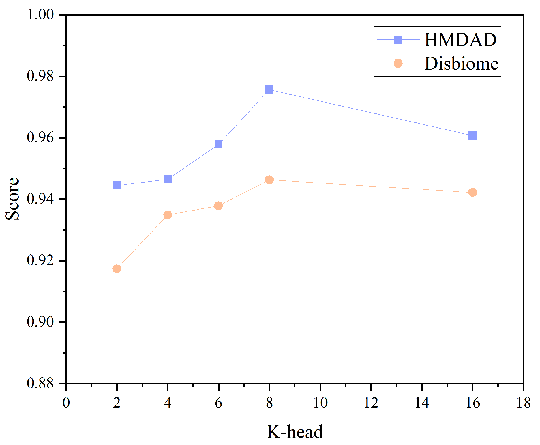
2.2.1. Multi-Head Attention Mechanism Calculation

To effectively capture the potential features between the microorganisms and diseases and measure the importance of the source node $V_d$ to the target node $V_m$, we map the source node $v_d$ to a Key vector and use a linear projection $K-Linea{r}_{\tau \left(v_d\right)}^i:{\mathbb{R}}^{dim}\to {\mathbb{R}}^{{\displaystyle \frac{dim}{h}}}$ to project the source node’s original spatial features. Similarly, for the target node $v_m$, we map it to a Query vector and use a linear projection $Q-Linea{r}_{\tau \left(v_m\right)}^i:{\mathbb{R}}^{dim}\to {\mathbb{R}}^{{\displaystyle \frac{dim}{h}}}$ to project the target node’s original spatial features. Here, h represents the number of attention heads, $H^{l-1}\left[v_d\right]$ denotes the feature representation of the node at the $l-1$ layer, and $dim$ refers to the dimensionality of $H^{l-1}\left[v_d\right]$.

$$K^i\left(v_d\right)=K-Linea{r}_{\tau \left(v_d\right)}^i\left(H^{l-1}\left[v_d\right]\right)$$

(11)

$$Q^i\left(v_m\right)=Q-Linea{r}_{\tau \left(v_m\right)}^i\left(H^{l-1}\left[v_m\right]\right)$$

(12)

By calculating the similarity between the Query and Key vectors, we obtain the attention weight $V_d$ for the source node $V_m$ to the target node ${\mathrm{ATT}}_{\mathrm{head}}(v_d,e_{dm},v_m)$.

$${\mathrm{ATT}}_{\mathrm{head}}^i(v_d,e_{dm},v_m)=\left(K^i\left(v_d\right)W_{\varphi \left(e_{dm}\right)}^{ATT}{Q}^i{\left(v_m\right)}^T\right)·{\displaystyle \frac{{\mu }_{\langle \tau \left(v_d\right),\varphi \left(e_{dm}\right),\tau \left(v_m\right)\rangle }}{\sqrt{dim}}}$$

(13)

Finally, the attention from h heads is concatenated, and a Softmax operation is applied to the attention weights of all source nodes $v_m$ for each target node $N\left(v_m\right)$ to obtain the attention vector from the source nodes to the target nodes.

$$AT{T}^l(v_d,e_{dm},v_m)=\underset{\forall v_d\in \mathcal{N}\left(v_m\right)}{Softmax}\left(\underset{\forall d\in N\left(d\right)}{\parallel }AT{T}_{hea{d}_i}^l(v_d,e_{dm},v_m)\right)$$

(14)

2.2.2. Message Passing and Aggregation

When calculating node attention, we transmit information from the source node to the target node. To address the differences in the distribution of different types of nodes and edges, this study incorporates the meta-relationship of edges into the message passing process. To obtain the i-th head message ${\mathrm{MSG}}_{\mathrm{head}}^i(v_d,e_{dm},v_m)$, the source node is projected into the i-th message vector with a linear projection $M-Linea{r}_{\tau \left(v_m\right)}^i:{\mathbb{R}}^{dim}\to {\mathbb{R}}^h$, and the edge dependencies are integrated through the matrix $W_{\mathrm{MSG}}\varphi \left(e_{dm}\right)\in {\mathbb{R}}^{h\times h}$.

$${\mathrm{MSG}}_{\mathrm{head}}^i(v_d,e_{dm},v_m)=M-Linea{r}_{\tau \left(v_m\right)}^i\left(H^{(l-1)}\left[v_d\right]\right)W_{\varnothing \left(e_{dm}\right)}^{MSG}$$

(15)

The multi-head information is combined to obtain the information vector for each node.

$$\mathrm{Message}(v_d,e_{dm},v_m)=\underset{i\in [1,h]}{\parallel }{\mathrm{MSG}}_{\mathrm{head}}^i(v_d,e_{dm},v_m)$$

(16)

After calculating the multi-head attention and message information, the information from all neighboring nodes with different feature distributions must be aggregated to the target node. In this study, the attention vector is used as the weight for the node information, and the messages from the source nodes are normalized to obtain the updated node feature vector $H^l\left[v_m\right]$. Here, ⨁ represents the concatenation of information.

$$H^l\left[v_m\right]=\underset{v_d\in N\left(v_m\right)}{⨁}\left(\mathrm{Attention}(v_d,e_{dm},v_m)·\mathrm{Message}(v_d,e_{dm},v_m)\right)$$

(17)

Finally, the target node vector is mapped back to its specific feature distribution. The node vector $A_{-}Linea{r}_{\tau \left(v_m\right)}^i$ is updated using a linear projection $H^l\left[v_m\right]$ and connected through a residual network.

$$H^l\left[v_m\right]=A_{-}Linea{r}_{\tau \left(v_m\right)}^i\left(\sigma \left(H^l\left[v_m\right]\right)+H^{(l-1)}\left[v_m\right]\right)$$

(18)

3. LightGBM Method

LightGBM is a machine learning framework based on gradient boosting decision trees (GBDT). It uses decision tree algorithms and applies gradient boosting to combine multiple trees in a weighted manner, solving both regression and classification problems [32,33]. The method employs two innovative techniques, Gradient-based One-Side Sampling (GOSS) and Exclusive Feature Bundling (EFB), which effectively enhance both the training efficiency and accuracy of the algorithm. These techniques enable LightGBM to significantly reduce training time when handling large-scale datasets, while maintaining high predictive performance.

GOSS is a method used by LightGBM to improve training efficiency by sampling samples with larger gradients. In traditional GBDT algorithms, training each tree is based on the gradient information from all samples. GOSS reduces the computational cost by sampling only those samples with larger gradients.

First, we calculate the gradient $g_i$, for each sample, and then select the samples with larger gradients using the following formula:

$$\mathrm{Sampling}\mathrm{Probability}\left(i\right)=\left\{\begin{array}{cc}{\displaystyle \frac{|g_i|}{{\sum }_{i=1}^n\left|g_i\right|}},\hfill & |g_i|>\delta \hfill \\ {\displaystyle \frac{|g_i|}{\delta }},\hfill & \mathrm{otherwise}\hfill \end{array}\right.$$

where $g_i$ is the gradient of the i sample, n is the number of samples, and $\delta$ is a predefined threshold. For samples with smaller gradients, a lower sampling probability is used, reducing their impact on the computation.

The EFB method aims to reduce the dimensionality of the feature space by bundling sparse features into exclusive features. This method is primarily used to handle sparse features—especially when the number of features is large—by combining features with similar information, thereby reducing the computational cost during training. In EFB, the similarity between each pair of features is calculated, and similar features are bundled together.

LightGBM uses the following histogram-based optimization method to accelerate gradient computation and reduce memory usage:

• Prediction Initialization: For each microbiome–disease pair, LightGBM initializes the predicted value using the mean of the training data labels.
• Gradient Calculation: For each training sample i, the gradient of the loss function is calculated as $g_i={\displaystyle \frac{\partial \mathcal{L}(y_i,f\left(x_i\right))}{\partial f\left(x_i\right)}}$, where $\mathcal{L}$ is the loss function, $y_i$ is the true label, and $f\left(x_i\right)$ is the predicted value.
• Decision Tree Construction: The GOSS sampling method is used to select samples with larger gradients, thereby accelerating the tree construction.
• Prediction Update: The output of the new tree is added to the existing predicted values, updating the predictions for the microbiome–disease pairs.
• Iterative Training: The model is iteratively optimized through gradient descent and multiple tree constructions until the preset number of trees is reached or error convergence occurs.

After training is complete, LightGBM outputs the probability $P(y=1|x)$ for each microbiome–disease pair, representing the likelihood that the microbiome is associated with the disease. The final prediction $\widehat{y}$ is classified based on the probability value, as expressed in the following equation:

$$\widehat{y}=\left\{\begin{array}{cc}1,\hfill & P(y=1|x)>0.5\hfill \\ 0,\hfill & P(y=1|x)\le 0.5\hfill \end{array}\right.$$

where $\widehat{y}$ is the predicted label; 1 indicates an association and 0 indicates no association.

4. Results

In this section, we evaluate the proposed HG-LGBM model on two datasets, HMDAD (http://www.cuilab.cn/hmdad accessed on 14 April 2025) and Disbiome (https://disbiome.ugent.be/home accessed on 14 April 2025), and compare its performance with existing methods such as DAEGCNDF, SAELGMDA, GATMDA, and MNNMDA. Furthermore, we conduct a detailed analysis of the model’s hyperparameters, exploring the impact of factors such as the number of layers, the number of attention heads, and LightGBM hyperparameters on model performance. The microbiome–disease benchmark datasets are shown in

Table 1. Dataset Statistics.

Datasets	Microbes	Diseases	Associations
HMDAD	292	39	450
Disbiome	1052	218	4351

.

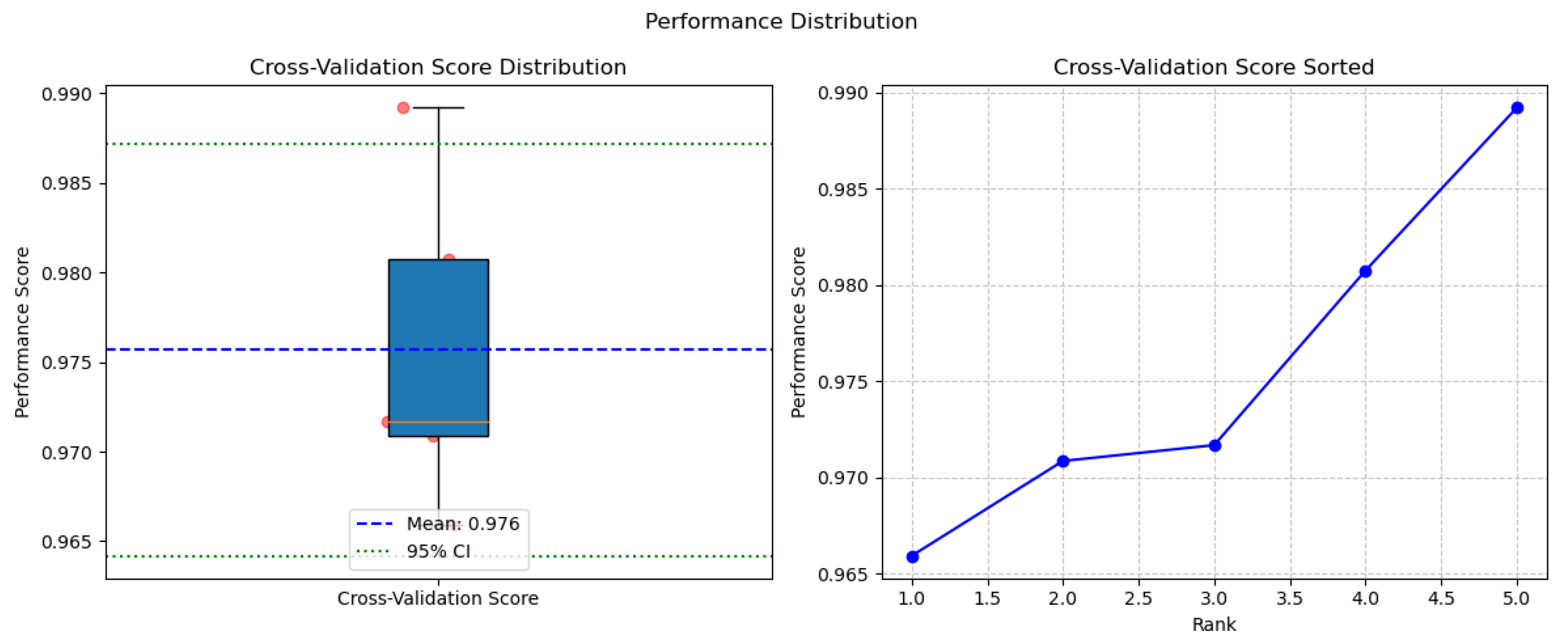
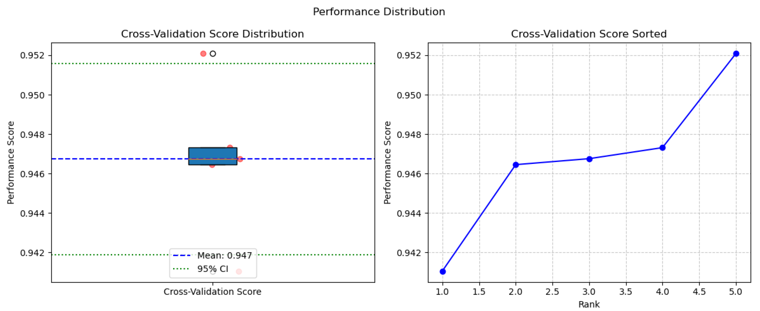
4.1. Performance Analysis

To comprehensively evaluate the model’s performance, we employed five-fold cross-validation by randomly dividing each dataset into five equal parts. Four parts were used for training the model, while the remaining part served as the test set to assess its predictive accuracy. As shown in

Table 2. Performance comparison of the HG-LGBM model on the HMDAD and Disbiome datasets.

Metric	HMDAD (Mean)	Disbiome (Mean)
AUC	0.9757	0.9463
AUPR	0.9711	0.9283
F1-score	0.9246	0.8868
Accuracy	0.9233	0.8836
Recall	0.9336	0.9126
Specificity	0.9123	0.8549
Precision	0.9162	0.8620

, the HG-LGBM model demonstrated strong discriminative performance across both datasets. On the HMDAD dataset, it achieved an AUC of $0.9757\pm 0.0032$, an F1-score of $0.9246\pm 0.0089$, and an accuracy of $0.9233\pm 0.0091$. On the Disbiome dataset, it attained an AUC of $0.9463\pm 0.0051$, an F1-score of $0.8868\pm 0.0123$, and an accuracy of $0.8836\pm 0.0131$. Additionally, the model’s statistical robustness was further confirmed through visual analyses using boxplots and rank performance charts, as illustrated in Figure 2 and Figure 3.

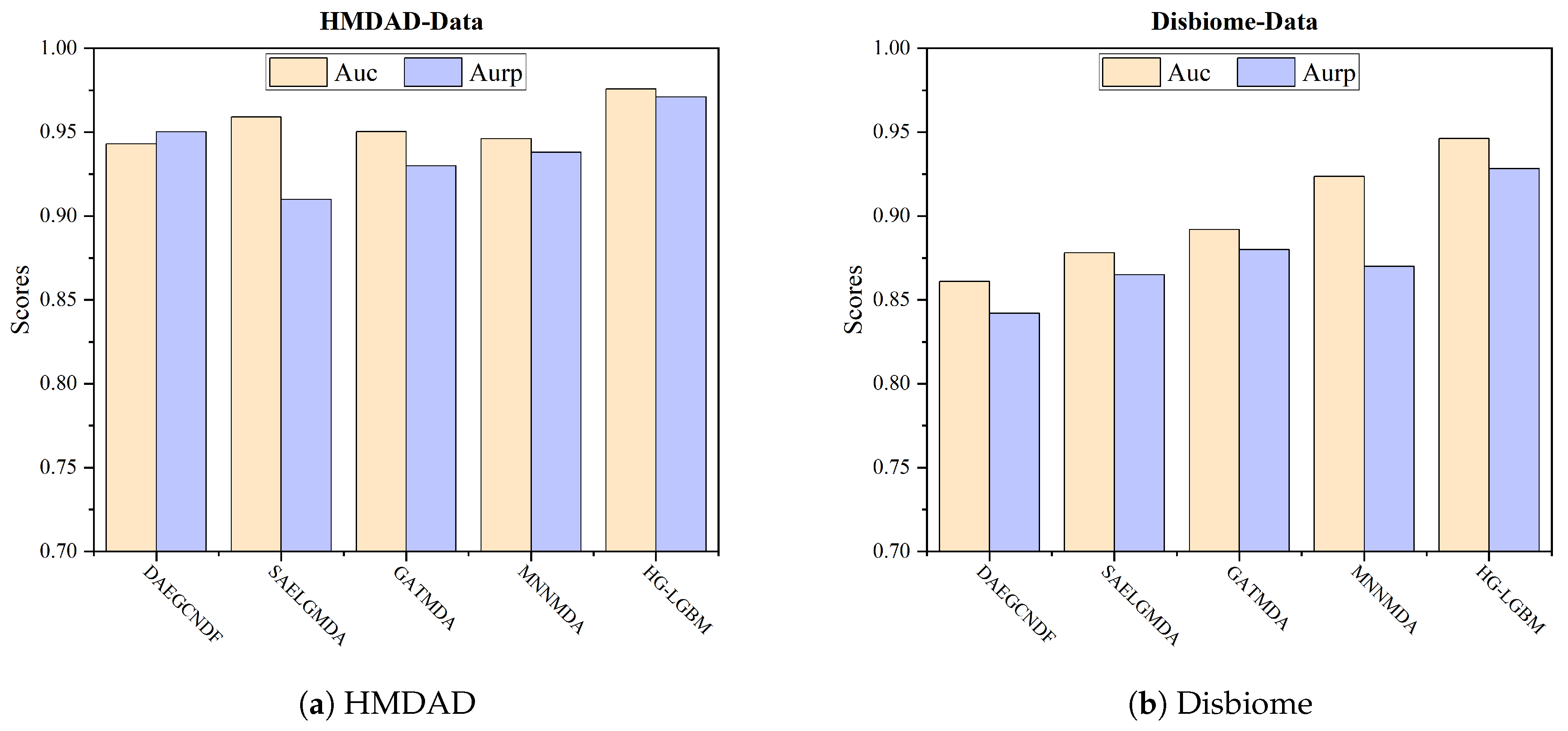
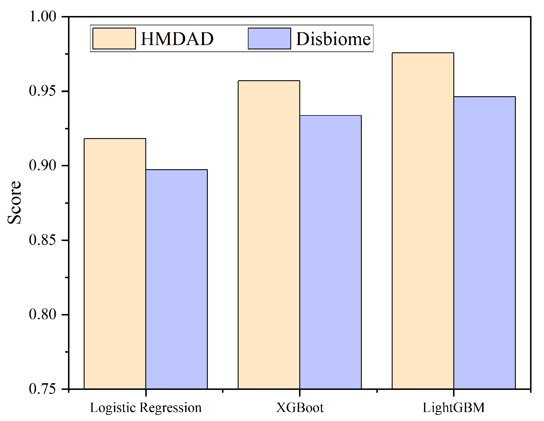
4.2. Model Comparison

To assess the predictive performance of the proposed HG-LGBM model, we selected the latest benchmark models in the microbiome–disease association prediction field that have an open-source code for comparison analysis. These include DAEGCNDF, which is based on deep autoencoder graph convolution, SAELGMDA, which integrates sparse autoencoding and graph attention, GATMDA, which uses the graph attention mechanism, and MNNMDA, which is based on matrix factorization. The performance comparison of each method on the HMDAD and Disbiome datasets is shown in Figure 4. The experimental results show that HG-LGBM demonstrates significant advantages on both benchmark datasets; the AUC value on the HMDAD dataset improved by 1.76% over the second-best model, SAELGMDA, and the prediction accuracy on the Disbiome dataset was 1.97% higher than that of MNNMDA. In microbiome disease data, there are significant semantic differences between node and edge types. HG-LGBM integrates the Heterogeneous Graph Transformer (HGT) with LightGBM, enabling the model to effectively capture the complex nonlinear relationships between microbes and diseases. The multi-head attention mechanism of HGT allows HG-LGBM to learn from various types of interactions within the heterogeneous network, while LightGBM’s gradient boosting method ensures the efficient classification of high-dimensional features. This combination enables HG-LGBM to enhance predictive accuracy and capture richer feature representations.

Additionally, we conducted comparative experiments on the Disbiome and HMDAD benchmark datasets, comparing the performance of our model with the XGBoost and Logistic Regression methods. The results are shown in Figure 5. Under most experimental conditions, LightGBM demonstrated superior predictive performance compared to XGBoost and Logistic Regression. The outstanding performance of LightGBM can be attributed to its efficient gradient boosting algorithm, support for large-scale parallel computing, and strong generalization capability. These features allow LightGBM to effectively avoid overfitting and provide more stable and reliable predictions when handling complex data, especially when dealing with high-dimensional features and large datasets. The comparison with XGBoost and Logistic Regression further highlights the superiority of LightGBM in microbiome–disease association prediction.

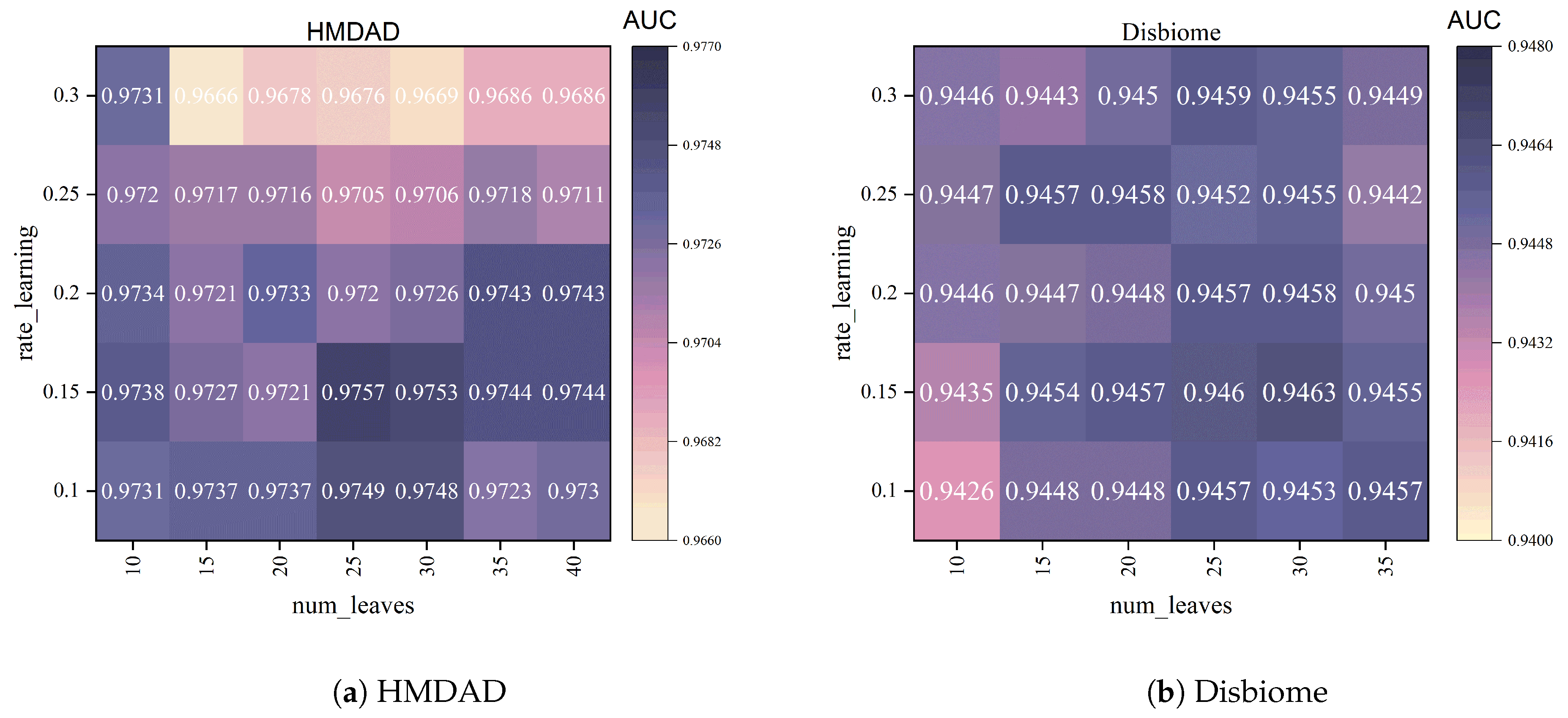
4.3. Hyperparameter Analysis

In this study, we conducted a detailed analysis of several hyperparameters of the HG-LGBM model, including the number of attention heads, the number of network layers, and LightGBM hyperparameters. These hyperparameters were optimized using the grid search and random search methods to ensure the model achieves optimal performance on the training set.

First, we investigated the impact of different numbers of attention heads on model performance. In the experiment, we tested configurations with 2, 4, 6, 8, and 16 heads. The results, shown in Figure 6, indicate that when the number of attention heads $K=8$, HG-LGBM achieved the best performance on the HMDAD and Disbiome datasets. Specifically, fewer heads (such as two and four heads) failed to capture the complex relationships between microorganisms and diseases, leading to a decrease in performance. While a larger number of heads (such as 16 heads) increased the model’s expressive power, too many attention heads introduced computational redundancy without significantly improving the model’s performance. Therefore, $K=8$ is able to capture the complex relationships between microorganisms and diseases to the fullest extent while maintaining computational efficiency.

Next, we conducted experiments to evaluate the impact of the depth of the Transformer layer on model performance, testing different network depths of two, four, six, and eight layers. The experimental results, shown in Figure 7, demonstrate that HG-LGBM provided the best performance for the microbiome–disease prediction task when the number of layers $h=6$. Shallow networks were unable to adequately capture the complex relationships in the task, resulting in lower prediction accuracy. Deeper networks, on the other hand, faced the risk of overfitting. Therefore, to balance model expressiveness with the prevention of overfitting, we selected $h=6$ as the optimal number of layers.

When optimizing the LightGBM hyperparameters, we focused on key parameters such as num_leaves, learning_rate, and max_depth. By adjusting and optimizing these parameters, we identified the optimal hyperparameter combination (num_leaves = 25, learning_rate = 0.15, max_depth = −1), ensuring robustness and efficiency across different datasets. The experimental results are shown in Figure 8.

• num_leaves: This parameter controls the number of leaves in a tree, affecting the model’s complexity. A larger num_leaves allows the model to be more flexible and learn more complex relationships, but it may lead to overfitting. A smaller num_leaves helps reduce overfitting, but it may limit the model’s expressiveness. We tested several different num_leaves values, including [5, 10, 15, 20, 25, 30, 35, 40], and ultimately selected num_leaves = 25, which showed the best balance on the validation set.
• learning_rate: This parameter represents the learning rate for model iteration. A higher learning rate can speed up convergence, but it may lead to instability and overfitting. A lower learning rate provides more stable training, but it may require more iterations to converge. We tested several learning_rate values (0.1, 0.15, 0.2, 0.25, 0.3) and ultimately selected learning_rate = 0.15, which provided the best balance between learning speed and prediction performance during training.
• max_depth: This parameter controls the maximum depth of each tree, which determines the tree’s complexity. If max_depth is set too deep, it may cause overfitting; if it is set too shallow, it may cause underfitting. In our experiments, we set max_depth = −1 to allow the model to adaptively determine the depth based on the data, better capturing complex patterns in the data.

5. Case Study

To further validate the biological significance and clinical application potential of the HG-LGBM model, this study conducted a detailed analysis of the prediction results for inflammatory bowel disease (IBD) and colorectal cancer (CRC) using the HMDAD dataset. By excluding known associated microorganisms and reviewing relevant publications in the biomedical database PubMed, we validated the associations between the diseases and microorganisms.

Microbial Association Analysis of Inflammatory Bowel Disease (IBD)

IBD refers to a group of chronic inflammatory bowel diseases, including Crohn’s Disease and Ulcerative Colitis. The dysbiosis of the gut microbiota plays a crucial role in the pathogenesis of IBD. This study presents the predicted associations of the top 10 microorganisms with IBD, as shown in

Table 3. Microbes related to IBD inferred by HG-LGBM on the HMDAD database.

Rank	Microbe	Evidence (PMID)
1	Veillonella	38980940
2	Prevotella	38053528
3	Bifidobacterium	38368394
4	Clostridium coccoides	26994772
5	Bacteroidetes	31071294
6	Klebsiella	38545880
7	Haemophilus	34334167
8	Firmicutes	35951774
9	Lactobacillus	37773196
10	Enterococcus	38788722

. Studies have confirmed that Veillonella and Prevotella are associated with intestinal inflammation. An increase in the abundance of Prevotella may exacerbate gut inflammation by activating host immune responses. Meanwhile, the metabolites of Veillonella (such as short-chain fatty acids) are significantly imbalanced in IBD patients, potentially affecting the intestinal mucosal barrier function. Additionally, Klebsiella, as an opportunistic pathogen, may promote inflammation by overgrowing and activating the Toll-like receptor 4 (TLR4) signaling pathway through lipopolysaccharides (LPSs). These results not only confirm the reliability of the model but also suggest that HG-LGBM can capture key features of the interaction between microbial function and host immunity.

Colorectal cancer (CRC) is the third most common cancer worldwide and is closely associated with the gut microbiota. The gut microbiota plays a crucial role in the onset and progression of CRC by modulating immune responses, producing metabolites, and altering gene expression. This study presents the predicted associations of the top 10 microorganisms with IBD, as shown in

Table 4. Microbes related to CRC inferred by HG-LGBM on the HMDAD database.

Rank	Microbe	Evidence (PMID)
1	Clostridium coccoides	26084032
2	Proteobacteria	37263983
3	Actinobacteria	38648753
4	Staphylococcus	36037202
5	Lachnospiraceae	36893736
6	Haemophilus	35663463
7	Lactobacillus	37192617
8	Collinsella aerofaciens	37704113
9	Enterococcus	35090978
10	Desulfovibrio	38484555

. Additionally, the literature indicates that Clostridium coccoides may promote DNA damage through the metabolism of secondary bile acids, while the enrichment of Proteobacteria is linked to increased oxidative stress in the gut microenvironment of CRC patients. Lachnospiraceae typically exhibits decreased abundance in CRC, and the reduction in its anti-inflammatory metabolites (such as butyrate) may lead to the abnormal proliferation of intestinal epithelial cells.

6. Conclusions

This study presents HG-LGBM, a computational framework that combines heterogeneous graph neural networks and gradient boosting techniques to predict the associations between microorganisms and diseases. By integrating multi-view similarity features and utilizing a hierarchical attention mechanism, the model effectively captures nonlinear relationships and network heterogeneity, successfully addressing the limitations of existing methods. The experimental results on benchmark datasets demonstrated that HG-LGBM significantly outperforms advanced methods such as GATMDA and MNNMDA, showcasing its exceptional performance. The model’s interpretability and scalability further highlight its potential in pathogen identification and therapeutic intervention. Future work will focus on integrating dynamic microbiome data and expanding the framework for multi-omics integration, aiming to enhance its application in complex disease diagnosis and microbiome-based therapies. This study advances computational strategies for understanding microbiome–disease relationships and accelerates progress in the field of gut microbiome–disease association research.

References

1. Aggarwal, N.; Kitano, S.; Puah, G.R.Y.; Kittelmann, S.; Hwang, I.Y.; Chang, M.W. Microbiome and Human Health: Current Understanding, Engineering, and Enabling Technologies. Chem. Rev. 2023, 123, 31–72. [Google Scholar] [CrossRef] [PubMed]
2. Fan, Y.; Pedersen, O. Gut microbiota in human metabolic health and disease. Nat. Rev. Microbiol. 2021, 19, 55–71. [Google Scholar] [CrossRef] [PubMed]
3. Chen, Y.; Fischbach, M.; Belkaid, Y. Skin microbiota–host interactions. Nature 2018, 553, 427–436. [Google Scholar] [CrossRef] [PubMed]
4. Hou, K.; Wu, Z.X.; Chen, X.Y.; Wang, J.Q.; Zhang, D.; Xiao, C.; Zhu, D.; Koya, J.B.; Wei, L.; Li, J.; et al. Microbiota in health and diseases. Signal Transduct. Target. Ther. 2022, 7, 135. [Google Scholar] [CrossRef]
5. Brown, J.; Hazen, S. Microbial modulation of cardiovascular disease. Nat. Rev. Microbiol. 2018, 16, 171–181. [Google Scholar] [CrossRef]
6. Sepich-Poore, G.D.; Zitvogel, L.; Straussman, R.; Hasty, J.; Wargo, J.A.; Knight, R. The microbiome and human cancer. Science 2021, 371, eabc4552. [Google Scholar] [CrossRef]
7. Wu, J.; Wang, K.; Wang, X.; Pang, Y.; Jiang, C. The role of the gut microbiome and its metabolites in metabolic diseases. Protein Cell 2021, 12, 360–373. [Google Scholar] [CrossRef]
8. Schirmer, M.; Garner, A.; Vlamakis, H.; Xavier, R.J. Microbial genes and pathways in inflammatory bowel disease. Nat. Rev. Microbiol. 2019, 17, 497–511. [Google Scholar] [CrossRef]
9. Stripling, J.; Rodriguez, M. Current evidence in delivery and therapeutic uses of fecal microbiota transplantation in human diseases-clostridium difficile disease and beyond. Am. J. Med. Sci. 2018, 356, 424–432. [Google Scholar] [CrossRef]
10. Benech, N.; Sokol, H. Fecal microbiota transplantation in gastrointestinal disorders: Time for precision medicine. Genome Med. 2020, 12, 58. [Google Scholar] [CrossRef]
11. Cunningham, M.; Vinderola, G.; Charalampopoulos, D.; Lebeer, S.; Sanders, M.E.; Grimaldi, R. Applying probiotics and prebiotics in new delivery formats—Is the clinical evidence transferable? Trends Food Sci. Technol. 2021, 112, 495–506. [Google Scholar] [CrossRef]
12. Kahouli, I.; Malhotra, M.; Westfall, S.; Alaoui-Jamali, M.A.; Prakash, S. Design and validation of an orally administrated active L. fermentum-L. acidophilus probiotic formulation using colorectal cancer Apc Min/+ mouse model. Appl. Microbiol. Biotechnol. 2017, 101, 1999–2019. [Google Scholar] [CrossRef] [PubMed]
13. Sasaki, M.; Ogasawara, N.; Funaki, Y.; Mizuno, M.; Iida, A.; Goto, C.; Koikeda, S.; Kasugai, K.; Joh, T. Transglucosidase improves the gut microbiota profile of type 2 diabetes mellitus patients: A randomized double-blind, placebo-controlled study. BMC Gastroenterol. 2013, 13, 81. [Google Scholar] [CrossRef]
14. Routy, B.; Le Chatelier, E.; Derosa, L.; Duong, C.P.; Alou, M.T.; Daillère, R.; Fluckiger, A.; Messaoudene, M.; Rauber, C.; Zitvogel, L.; et al. Gut microbiome influences efficacy of PD-1-based immunotherapy against epithelial tumors. Science 2018, 359, 91–97. [Google Scholar] [CrossRef]
15. Qi, X.; Li, X.; Zhao, Y.E.; Wu, X.; Chen, F.; Ma, X.; Zhang, F.; Wu, D. Treating steroid refractory intestinal acute graft-vs.-host disease with fecal microbiota transplantation: A pilot study. Front. Immunol. 2018, 9, 2195. [Google Scholar] [CrossRef]
16. Morton, J.T.; Aksenov, A.A.; Nothias, L.F.; Foulds, J.R.; Quinn, R.A.; Badri, M.H.; Swenson, T.L.; Goethem, M.W.V.; Northen, T.R.; Knight, R.; et al. Learning representations of microbe–metabolite interactions. Nat. Methods 2019, 16, 1306–1314. [Google Scholar] [CrossRef]
17. Jiang, C.; Feng, J.; Shan, B.; Chen, Q.; Yang, J.; Wang, G.; Peng, X.; Li, X. Predicting microbe-disease associations via graph neural network and contrastive learning. Front. Microbiol. 2024, 15, 1483983. [Google Scholar] [CrossRef]
18. Chen, X.; Huang, Y.-A.; You, Z.-H.; Yan, G.-Y.; Wang, X.-S. A novel approach based on KATZ measure to predict associations of human microbiota with non-infectious diseases. Bioinformatics 2017, 33, 733–739. [Google Scholar] [CrossRef]
19. Huang, Z.-A.; Chen, X.; Zhu, Z.; Liu, H.; Yan, G.-Y.; You, Z.-H.; Wen, Z. PBHMDA: Path-Based Human Microbe-Disease Association Prediction. Front. Microbiol. 2017, 8, 233. [Google Scholar] [CrossRef]
20. Chen, Y.; Lei, X. Metapath Aggregated Graph Neural Network and Tripartite Heterogeneous Networks for Microbe-Disease Prediction. Front. Microbiol. 2022, 13, 919380. [Google Scholar] [CrossRef]
21. Zou, S.; Zhang, J.; Zhang, Z. A novel approach for predicting microbe-disease associations by bi-random walk on the heterogeneous network. PLoS ONE 2017, 12, e0184394. [Google Scholar] [CrossRef] [PubMed]
22. He, B.-S.; Peng, L.-H.; Li, Z. Human Microbe-Disease Association Prediction With Graph Regularized Non-Negative Matrix Factorization. Front. Microbiol. 2018, 9, 2560. [Google Scholar] [CrossRef] [PubMed]
23. Liu, H.; Bing, P.; Zhang, M.; Tian, G.; Ma, J.; Li, H.; Bao, M.; He, K.; He, J.; He, B.; et al. MNNMDA: Predicting human microbe-disease association via a method to minimize matrix nuclear norm. Comput. Struct. Biotechnol. J. 2023, 21, 1414–1423. [Google Scholar] [CrossRef] [PubMed]
24. Zitnik, M.; Nguyen, F.; Wang, B.; Leskovec, J.; Goldenberg, A.; Hoffman, M.M. Machine learning for integrating data in biology and medicine: Principles, practice, and opportunities. Inf. Fusion 2019, 50, 71–91. [Google Scholar] [CrossRef]
25. Wang, F.; Yang, H.; Wu, Y.; Peng, L.; Li, X. SAELGMDA: Identifying human microbe–disease associations based on sparse autoencoder and LightGBM. Front. Microbiol. 2023, 14, 1207209. [Google Scholar] [CrossRef]
26. Long, Y.; Luo, J.; Zhang, Y.; Xia, Y. Predicting human microbe–disease associations via graph attention networks with inductive matrix completion. Brief. Bioinform. 2021, 22, bbaa146. [Google Scholar] [CrossRef]
27. Lu, S.; Liang, Y.; Li, L.; Miao, R.; Liao, S.; Zou, Y.; Yang, C.; Ouyang, D. Predicting potential microbe-disease associations based on auto-encoder and graph convolution network. BMC Bioinform. 2023, 24, 476. [Google Scholar] [CrossRef]
28. Gong, H.; You, X.; Jin, M.; Meng, Y.; Zhang, H.; Yang, S.; Xu, J. Graph neural network and multi-data heterogeneous networks for microbe-disease prediction. Front. Microbiol. 2022, 13, 1077111. [Google Scholar] [CrossRef]
29. Wen, S.; Liu, Y.; Yang, G.; Chen, W.; Wu, H.; Zhu, X.; Wang, Y. A method for miRNA-disease association prediction using machine learning decoding of multi-layer heterogeneous graph Transformer encoded representations. Sci. Rep. 2024, 14, 20490. [Google Scholar] [CrossRef]
30. Kamneva, O.K. Genome composition and phylogeny of microbes predict their co-occurrence in the environment. PLoS Comput. Biol. 2017, 13, e1005366. [Google Scholar] [CrossRef]
31. Van Laarhoven, T.; Nabuurs, S.B.; Marchiori, E. Gaussian interaction profile kernels for predicting drug–target interaction. Bioinformatics 2011, 27, 3036–3043. [Google Scholar] [CrossRef] [PubMed]
32. Cheng, C.; Zhang, Q.; Ma, Q.; Yu, B. LightGBM-PPI: Predicting protein-protein interactions through LightGBM with multi-information fusion. Chemom. Intell. Lab. Syst. 2019, 191, 54–64. [Google Scholar] [CrossRef]
33. Shaker, B.; Yu, M.S.; Song, J.S.; Ahn, S.; Ryu, J.Y.; Oh, K.S.; Na, D. LightBBB: Computational prediction model of blood–brain-barrier penetration based on LightGBM. Bioinformatics 2020, 37, 1135–1139. [Google Scholar] [CrossRef] [PubMed]
Figure 1. The flowchart of HG-LGBM.
Applsci 15 04452 g001
Figure 2. Boxplot and rank performance chart of the HG-LGBM model on the HMDAD dataset, illustrating its statistical robustness.
Applsci 15 04452 g002
Figure 3. Boxplot and rank performance chart of the HG-LGBM model on the Disbiome dataset, illustrating its statistical robustness.
Applsci 15 04452 g003
Figure 4. The performance of HMDAD with all comparsion methods.
Applsci 15 04452 g004
Figure 5. The performance of three classification models.
Applsci 15 04452 g005
Figure 6. The performance of different heads.
Applsci 15 04452 g006
Figure 7. The performance of different layers.
Applsci 15 04452 g007
Figure 8. The performance of HMDAD with all comparison methods.
Applsci 15 04452 g008