Predicting Noise and User Distances from Spectrum Sensing Signals Using Transformer and Regression Models

Abstract

Frequency spectrum allocation has been a subject of dispute in recent years. Cognitive radio dynamically allocates users to spectrum holes using various sensing techniques. Noise levels and distances between users can significantly impact the efficiency of cognitive radio systems. Designing robust communication systems requires accurate knowledge of these factors. This paper proposes a method for predicting noise levels and distances based on spectrum sensing signals using regression machine learning models. The proposed methods achieved correlation coefficients of over $0.98$ and $0.82$ for noise and distance predictions, respectively. Accurately estimating these parameters enables adaptive resource allocation, interference mitigation, and improved spectrum efficiency, ultimately enhancing the performance and reliability of cognitive radio networks.

1. Introduction

The frequency spectrum, essential for wireless communications, is a limited resource that has become increasingly congested [1,2,3]. Cognitive radio (CR) dynamically allocates communication for secondary users (SUs) in parts of the spectrum, known as spectrum holes, where primary users (PUs) are absent [4,5,6]. Several techniques exist for spectrum sensing, including energy detection, feature detection, Nyquist and sub-Nyquist methods, and multi-bit and one-bit compressive sensing. More recently, machine learning models have been employed to detect the presence of PUs [7,8]. Across these methods, noise can adversely affect the accurate detection of PUs, impacting the efficient use of the spectrum. In multi-user systems, the distance between users significantly influences the noise levels. Thus, predicting the noise level in the received signal and understanding user distances is fundamental for optimizing spectrum efficiency.

In communication systems, noise refers to any unwanted or random interference that compromises the quality of a transmitted signal. Noise can distort the original information being transmitted, leading to errors, diminished signal clarity, and reduced communication performance [9]. Almost all communication channels and systems encounter noise, which can originate from various sources. The noise level can be influenced by several factors, including transmitted power, path loss, shadow fading, multipath fading, and the distance between users. In addition to these factors, additive white Gaussian noise is a type of noise that exists across all frequencies [10]. This noise is characterized by its randomness and uniform energy distribution throughout the frequency spectrum. White Gaussian noise is a common model for representing random background noise in communication systems. By predicting noise levels, one can more effectively optimize system parameters and frequency allocation [11].

The distance between users is an important factor that influences signal quality and, consequently, spectrum efficiency. In spectrum sensing, the strength of the received signal depends on the distance between the transmitter and receiver. Predicting these distances helps to adjust the transmission power levels: users closer to the transmitter require lower power for reliable communication, while users farther away need higher power [12]. This power control optimizes energy efficiency and minimizes interference. Especially in systems with limited resources, such as bandwidth, predicting distances is fundamental for effective resource allocation. Users closer to the transmitter can be assigned greater bandwidth and consequently higher data rates, while those farther away might be allocated smaller bandwidths to improve the signal quality at the same transmission power level. Additionally, distance prediction is essential for providing location-based services. The distance between users can also impact the performance of artificial intelligence models used to increase spectrum efficiency. By estimating distances, services like navigation, location-based advertisements, and emergency services can be offered.

To predict noise and distances between users, regression models and deep learning architectures are recommended [13]. Regression models are a class of machine learning algorithms designed to predict continuous numerical values based on input data. These models play a crucial role in various fields, including economics, finance, healthcare, and natural sciences. They allow for the analysis and forecasting of trends, relationships, and outcomes by learning from historical data. Among the most common traditional machine learning regression approaches are support vector regression (SVR) (an extension of support vector machines to regression), decision trees and random forests [14], linear regression (one of the simplest yet most widely used regression techniques), and ridge and lasso regression (variants of linear regression). In more robust regression approaches, convolutional neural networks (CNNs), initially designed for image analysis, can be adapted for regression tasks [15]. More recently, transformer, designed for forecasting, has shown promise for regression activities [16].

In this article, we propose the use of regression models to predict noise levels and distances based on spectrum sensing signals. During our study, we generated a dataset that considers important parameters, including a wide range of noise power densities, an extensive sensing area, and power leakage from the PUs. We compared both traditional and deep learning models for prediction purposes. Furthermore, we evaluated the results using various metrics. Our proposed method has shown promising results, with a correlation coefficient exceeding 0.98 for noise and over 0.82 for distance. Additional metrics also indicate that our method is effective in predicting noise levels and distances between users. Such predictive capability can be important in designing communication systems to enhance spectrum efficiency.

This article is organized as follows: in Section 2, related works about the prediction of noise levels and distances between users in a communication system are presented; in Section 3, the proposed methodology for data generation, training, and evaluation is described; in Section 4, the experiments conducted and the results achieved are presented; the discussions related to the experiments are presented in Section 5; lastly, in Section 6, the conclusions are presented.

Contributions

The main contributions of this paper can be summarized as follows: (1) the use of the transformer model, one of the newest and most robust networks, which achieved good results for distance prediction even with a limited architecture; (2) for noise prediction, the classical regression methods presented excellent results, achieving a correlation coefficient greater than 0.98, demonstrating a high level of similarity between the predictions and real values; (3) since the current models used for spectrum sensing are very sensitive to signal quality, the proposed approach can help in designing better communication systems based on artificial intelligence models by providing prior information.

2. Related Works

In this section, the related works regarding noise and distance in terms of user prediction in a spectral sensing scheme are described in detail.

2.1. Noise Prediction

The authors proposed a signal-to-noise ratio (SNR) estimation method based on the sounding reference signal (SRS) and a deep learning network in [17]. The proposed deep learning network, called the denoising and image restoration network (DINet), combines a denoising convolutional neural network (DnCNN) and an image restoration convolutional neural network (IRCNN) in parallel. The method was compared to other algorithms, and the results demonstrated superior performance in SNR estimation. The evaluation metric used was the normalized mean square error (NMSE) calculated over 200 test samples, yielding an NMSE value of 0.0012. This result was significantly better than the performance achieved by other algorithms.

In [11], the authors presented a method for estimating SNR in long-term evolution (LTE) systems and fifth-generation (5G) networks. They employed a combination of a CNN and long short-term memory (LSTM), known as a CNN–LSTM neural network. The CNN was utilized to extract spatial features, while the LSTM was used to extract temporal features from the input signal. Data were generated using MATLAB R2020b LTE and 5G toolboxes, taking into consideration modulation types, path delays, and Doppler shifts. The evaluation metric used was NMSE. The NMSE achieved a value of zero in the time domain for SNR ranging from $-4$ to 32 dB, demonstrating very low latency. However, in the frequency domain, the proposed method exhibited lower performance.

In [18], the authors proposed a noise denoising residual network (NDR-Net), a novel neural network for channel estimation in the presence of unknown noise levels. NDR-Net comprises a noise level estimation subnet (NLES), a DnCNN, and a residual learning cascade (RLC). The NLES determines the noise interval, followed by the DnCNN, which processes the pure noise image. Subsequently, RLC is applied to extract the noiseless channel image. The evaluation metric used for assessing the model’s performance was the mean square error. The experiments conducted across different channel models—tapped delay line-A (TDL-A), TDL-B, and TDL-C—consistently demonstrated low mean square error values. However, it is worth noting that the proposed model’s performance was evaluated within an SNR range of 0 to 35 dB. This limited range does not provide a comprehensive understanding of the model’s robustness, particularly in scenarios with high levels of noise.

In

Table 1. Related works on noise prediction.

Reference	Research Direction	Contributions	Limitations
[17]	SNR estimation method based on SRS and a deep learning network	Proposed a DINet for SNR estimation, which is a DnCNN and IRCNN in parallel	The number of testing samples is small
[11]	Method for estimating SNR in LTE systems and 5G	They used a CNN–LSTM neural network to extract spatial and temporal features	The proposed method exhibited lower performance in the frequency domain
[18]	Novel neural network for channel estimation in the presence of unknown noise levels	Proposed an NDR-Net for channel estimation, which comprises an NLES, a DnCNN, and an RLC	Limited to a small range of noise levels
Proposed	Prediction of noise power density in spectrum sensing signals	Proposed several regression algorithms for predicting noise power density in signals, considering several other variables that influence the quality of the signal	Computing power was a limitation for training with more data and robust architectures

, some techniques for noise prediction are summarized and compared. The methodology proposed in this article considers several variables that influence signal quality for data generation. The study incorporates noise power density across a wide range of values and explores a spectrum sensing environment where multiple users are in motion at fixed speeds over time. Several regression models are compared using various metrics to highlight the robustness of the proposed method.

2.2. Distance Prediction

In [19], the authors proposed a deep learning approach for user equipment positioning in non-line-of-sight scenarios. The impact of variables such as the type of radio data, the number of base stations, the size of the training dataset, and the generalization of the trained models on third-generation partnership project (3GPP) indoor factory scenarios was analyzed. The model trained consisted of a customized residual neural network (ResNet) for the path gain dataset and ResNet-18 for the channel impulse response dataset. The metric used was the $90\%$ quantile of the cumulative distribution function of the horizontal positioning error. The authors obtained the best performance with a large number of samples for training and tuning the models.

In [20], the authors proposed a machine learning algorithm for indoor fingerprint positioning based on measured 5G signals. The dataset was created by collecting 5G signals in the positioning area and processing them to form fingerprint data. A CNN was trained to locate a 5G device in an indoor environment. The metrics used were the root mean square error and the circular error probable. The experiments were conducted in a real field and demonstrated a positioning accuracy of 96% for the proposed method.

Finally, in [21], the authors introduced a location-aware predictive beamforming approach utilizing deep learning techniques for tracking unmanned aerial vehicle communication beams in dynamic scenarios. Specifically, they designed a recurrent neural network called a location-aware recurrent network (LRNet), based on LSTM, to accurately predict unmanned aerial vehicle locations. Using the predicted location, it was possible to determine the angle between the unmanned aerial vehicle and the base station for efficient and rapid beam alignment in the subsequent time slot. This ensures reliable communication between the unmanned aerial vehicle and the base station. The simulation results demonstrate that the proposed approach achieves a highly satisfactory unmanned aerial vehicle to base station communication rate, approaching the upper limit attained by a perfect genie-aided alignment scheme.

In

Table 2. Related works on distance prediction.

Reference	Research Direction	Contributions	Limitations
[19]	User equipment positioning in non-line-of-sight scenarios	Proposed customized ResNet for the path gain dataset and ResNet-18 for the channel impulse response dataset	Without finetuning and with large number of samples, the models exhibited lower performance
[20]	Indoor fingerprint positioning based on measured 5G signals	A CNN was trained to locate a 5G device in an indoor environment. The experiments were conducted in a real field and demonstrated a positioning accuracy of 96% for the proposed method	The proposed method is not compared with other deep learning models
[21]	Location-aware predictive beamforming approach utilizing deep learning techniques for tracking unmanned aerial vehicle communication beams in dynamic scenarios	Designed a recurrent neural network called LRNet, based on LSTM, to accurately predict unmanned aerial vehicle locations. Using the predicted location, it was possible to determine the angle between the unmanned aerial vehicle and the base station for efficient and rapid beam alignment in the subsequent time slot	Limited only to unmanned aerial vehicle to base station communication
Proposed	Prediction of initial and final distances between users during spectrum sensing	Proposed several regression algorithms for predicting distances between users considering several other variables that influence the quality of the signal	Computing power was a limitation for training with more data and robust architectures

, some techniques for distance prediction are summarized and compared. The methodology proposed in this article considers several variables that influence signal quality for data generation. The study incorporates Euclidean distances between users across a wide range of values and explores a spectrum sensing environment where multiple users are in motion at fixed speeds over time. Several regression models are compared using various metrics to highlight the robustness of the proposed method.

3. Methods

This section presents the proposed methods for data generation and noise and distance predictions.

3.1. System Model

The use of generated data simulating PU signals is proposed in spectrum sensing to predict the noise level of the sensed signal and the initial and final distances between users. For this, the methodology is divided as follows: (1) database generation, where the signals that represent PUs are generated [1,2]; (2) training the proposed regression models [22,23]; and (3) evaluation of the trained models for predicting noise level and distance [13,24]. At the end of the process, it is expected that the models will be able to predict the level of noise and the initial and final distances between the PU and SU during the sensing period.

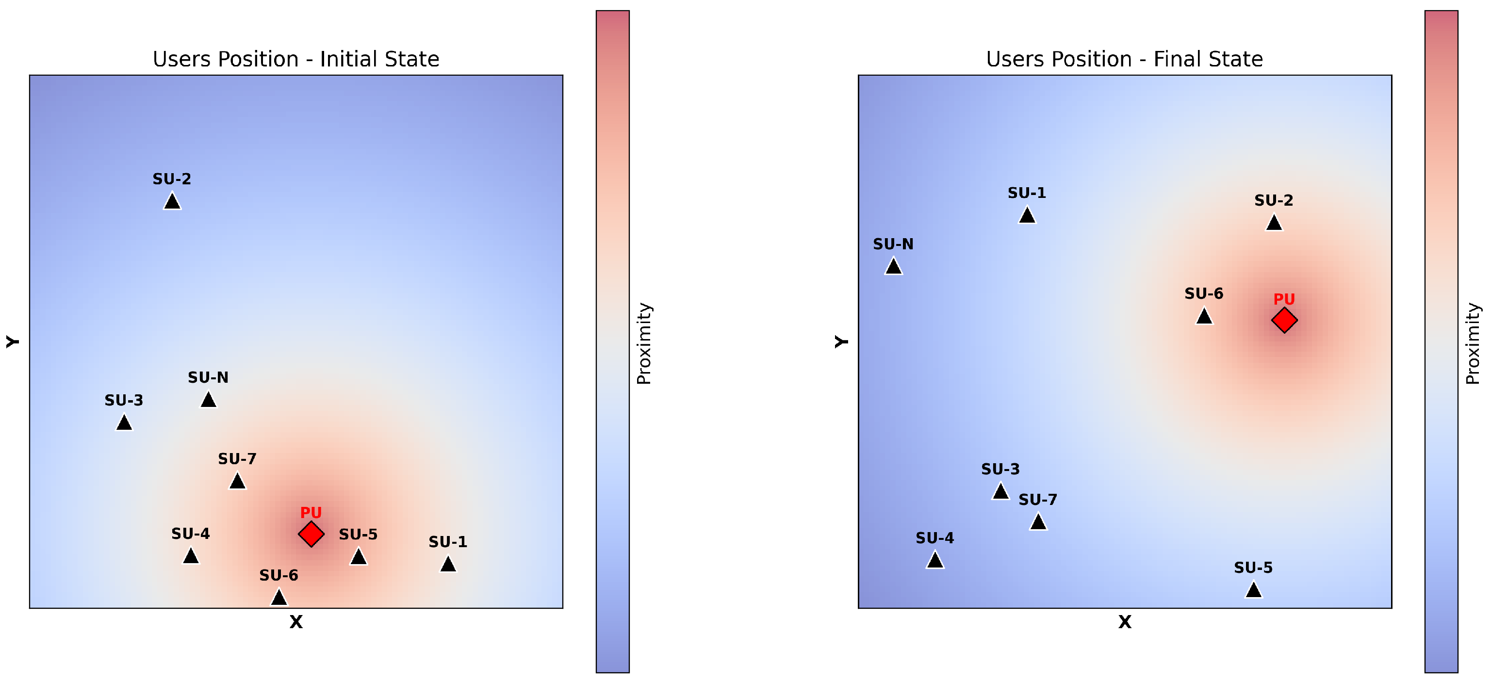
The dataset utilized for training the proposed regression models comprises signal data, noise levels, and distances between the users. Initially, the SU and PU are positioned within the area $X\times Y$, moving randomly for a duration of $\Delta t$. During this time, signals are sensed, and data on noise levels ($N_0$) as well as initial ($D_i$) and final ($D_f$) distances are collected. These collected data are then used to train and test the proposed regression models. To validate the effectiveness of the method in predicting noise levels and distances, various metrics are calculated.

Figure 1 illustrates the representation of the environment just described. The initial state (left) is an example of how users can be positioned within the area, while the final state (right) demonstrates the change in position after $\Delta t$. The PU, marked by a red diamond, and the SUs, represented by black triangles, are randomly positioned within the area. In the initial state, the heatmap represents the distance of each SU from the PU, with warmer (red) areas indicating closer proximity and cooler (blue) areas showing greater distances. In the final state, we can observe that the PU and SUs have changed positions, and the distances between the SUs may also vary during the observation period.

The output of step (1) is expected to be the signals that represent the PU, the associated noise level for each signal, and the initial and final distances during the sensing. Using this information, two regression models are trained: one for noise level prediction and another for initial and final distance predictions. In step (2), some classical machine learning regression models are employed, including random forest, decision tree, extra trees, XGBosst, LightGBM, SVR, and transformer. The output of this step consists of predicted values for noise level and distances given a test dataset. Lastly, in step (3), several metrics are used to evaluate the best models for these tasks.

3.2. Data Generation

In the spectrum sensing process, the decision on the channel condition is binary, involving two hypotheses: $H_1$ and $H_0$ [25]. Here, $H_1$ represents the hypothesis in which the PU is present, while $H_0$ represents the absence of the PU [2]. For the purposes of this paper, we will only consider hypotheses involving the presence of the PU. We assume that $N_{SU}$ SU and a single PU are moving at a speed v, with their starting positions randomly chosen within a given area. As a result, the users’ locations change over a time interval of $\Delta t$. Additionally, we are considering a multi-channel system with $N_B$ bands, each having a bandwidth of $B_W$. Furthermore, we assume that the PU can utilize $N_{B_P}$ consecutive bands [1]. Therefore, the received signal of the i-th SU on the j-th band at time n can be described as

$$y_i^j\left(n\right)=\left\{\begin{array}{cc}{s}_i^j\left(n\right)+w_i^j\left(n\right),& for{H}_{1}andj\in B_P\\ \sqrt{\eta }{s}_i^j\left(n\right)+w_i^j\left(n\right),& for{H}_{1}andj\in B_A\end{array}\right.$$

(1)

where $s_i^j\left(n\right)={\kappa }_i\left(n\right)g_i^j\left(n\right)x\left(n\right)$ and $w_i^j\left(n\right)$ is the additive white Gaussian noise (AWGN), whose noise power density is $N_0$, mean zero, and standard deviation $\sigma =\sqrt{B_W{10}^{{\displaystyle \frac{N_0}{10}}}}$. With $\eta$ being the proportion of power leaked to adjacent bands, $B_P$ represents the bands occupied by the PU and $B_A$ indicates the bands affected by the leaked power of the PU.

In the expression $s_i^j\left(n\right)$, a simplified path loss model is utilized, which can be written as follows:

$${\kappa }_i\left(n\right)=\sqrt{{\displaystyle \frac{P}{\beta {\left(d_i\left(n\right)\right)}^{\alpha }{10}^{\frac{h_i\left(n\right)}{10}}}}},$$

(2)

where $\alpha$ and $\beta$ denote the path-loss exponent and path-loss constant, respectively. Here, $d_i\left(n\right)$ represents the Euclidean distance between the PU and SU i at time n. The shadow fading of the channel, indicated by $h_i\left(n\right)$, between the PU and SU i at time n in decibels (dB) can be described by a normal distribution with a mean of zero and a variance of ${\sigma }^2$. The term P denotes the power transmitted by the PU within a specified frequency band. Furthermore, the multipath fading factor, denoted as $g_i^j\left(n\right)$, is modeled as an independent zero-mean circularly symmetric complex Gaussian (CSCG) random variable. Moreover, the data transmitted at time n, represented by $x\left(n\right)$, have an expected value of one [1,2].

3.3. Regression Models

The machine learning regression models used to predict interference and distance between the PU and SUs are random forest, decision tree, extra trees, XGBoosting, LightGBM, SVR, and transformer.

3.3.1. Random Forest

Random forest consists of a collection of trees denoted as $h(x;{\theta }_k),k=1,\dots ,K$. Here, x represents an input vector of length q, containing a correlated random vector X, while ${\theta }_k$ refers to independent and identically distributed random vectors. In the context of regression, assume that the observed data are drawn independently from the joint distribution of $(X,Y)$, where Y represents the numerical outcome. This dataset includes $n(q+1)$-tuples, namely $(x_1,y_1),\dots ,(x_n,y_n)$ [26]. The prediction of the random forest regression is the unweighted average over the collection

$$h\left(x\right)={\displaystyle \frac{1}{K}}\sum _{k=1}^{K}h(x;{\theta }_k)$$

(3)

3.3.2. Decision Tree

In the context of regression, the decision tree is based on recursively partitioning the input feature space into regions and then assigning a constant value to each region. This constant value serves as the prediction for any data point that falls within that region. Assume that X is the input data, Y the target variable, and $\theta$ represents the parameters that define the splits in the decision tree [27]. Let $h(X;\theta )$ be the predicted value for Y given input X and parameter $\theta$. Given a set of n training samples $(X_i,Y_i)$, where $i=1,2,\dots ,n$, the decision tree regressor seeks to find optimal split $\theta$ that minimizes the sum of square differences between the predicted value and the actual target value. The prediction for a given X can be represented as

$$h(X;\theta )=\sum _{i=1}^N{c}_{i}I(X\in R_i)$$

(4)

where N is the number of leaf nodes (regions) in the tree, $c_i$ is the constant value associated with the leaf node $R_i$, and $I(X\in R_i)$ is an indicator function that equals 1 if X falls within the region $R_i$ and 0 otherwise.

3.3.3. Extra Trees

The extra trees approach follows the same step-by-step process as random forest, using a random subset of features to train each base estimator [26], although the best feature and the corresponding value for splitting the node are randomly selected [28]. Random forest uses a bootstrap replica to train the model, while, with extra trees, the whole training dataset is used to train each regression tree [29].

3.3.4. XGBoosting

XGBoosting (XGB) is a highly optimized distributed gradient boosting library. It employs a recursive binary splitting strategy to identify the optimal split at each stage, leading to the construction of the best possible model [30]. Due to its tree-based structure, XGB is robust to outliers and, like many boosting methods, is effective in countering overfitting, making model selection more manageable. The regularized objective of the XGB model during the tth training step [31] is illustrated in Equation (5). Here, $l(y_{pred}^{\left(t\right)},y_{truth})$ represents the loss, which quantifies the disparity between the prediction of the imputed missing value $y_{pred}^{\left(t\right)}$ and the corresponding ground truth $y_{truth}$.

$$L^{\left(t\right)}=\sum _{i}l(y_{pred}^{\left(t\right)},y_{truth})+\sum _k\Omega \left(f_k\right)$$

(5)

where $\Omega \left(f_k\right)$ is the regularizer representing the complexity of the kth tree.

3.3.5. LightGBM

LightGBM (LGBM) is the gradient boosting decision tree (GBDT) algorithm with gradient-based one-side sampling (GOSS) and exclusive feature bundling (EFB). The GOSS technique is employed within the context of gradient boosting, utilizing a training set consisting of n instances {$x_1,\dots ,x_n$}, where each instance $x_i$ represents an s-dimensional vector in space ${\chi }^s$. In every iteration of gradient boosting, we compute the negative gradients of the loss function relative to the model’s output, resulting in {$g_1,\dots ,g_n$}. These training instances are then arranged in descending order, based on the absolute values of their gradients, and we select the top-$a\times 100\%$ instances with the largest gradient magnitudes to constitute a subset A [32]. For the complementing set $A^c$, comprising $(1-a)\times 100\%$ of instances characterized by smaller gradients, a random subset B is extracted, sized at $b\times \left|A^c\right|$. The division of instances is subsequently determined by the estimated variance gain concerning vector $V_j\left(d\right)$ over the combined subset $A\cup B$, where

$$V_j\left(d\right)={\displaystyle \frac{1}{n}}\left({\displaystyle \frac{{({\sum }_{x_i\in A_l}{g}_i+\frac{1-a}{b}{\sum }_{x_i\in B_l}{g}_i)}^2}{n_l^j\left(d\right)}}+{\displaystyle \frac{{({\sum }_{x_i\in A_r}{g}_i+\frac{1-a}{b}{\sum }_{x_i\in B_r}{g}_i)}^2}{n_r^j\left(d\right)}}\right)$$

(6)

where $A_l=\{x_i\in A:x_{ij}\le d\}$, $A_r=\{x_i\in A:x_{ij}>d\}$, $B_l=\{x_i\in B:x_{ij}\le d\}$, $B_r=\{x_i\in B:x_{ij}>d\}$, and ${\displaystyle \frac{1-a}{b}}$ is the coefficient used to normalize the the sum of the gradients over B back to the size of $A^c$.

3.3.6. SVR

Given n training data $(X_i,Y_i)$, $i=1,2,\dots ,n\subset \chi \times \mathbb{R}$, and $\chi$ represents the space of the input patterns [33]. The goal of the $\epsilon$-SVR is to find a function that exhibits a maximum deviation of $\epsilon$ or less from the target value $y_i$ obtained during training while also maintaining a minimal degree of fluctuation or variability. This function can be described as

$$f\left(x\right)=\langle w,x\rangle +b,\mathrm{with}w\in \chi ,b\in \mathbb{R}$$

(7)

where $\langle ·,·\rangle$ denotes dot product in $\chi$.

3.3.7. Transformer

A transformer model consists of an encoder and a decoder, each composed of multiple layers of self-attention and feed-forward neural networks. The base structure of a transformer is the self-attention mechanism. Given an input sequence, the self-attention computes a weighted sum of the values. Multi-head attention is used to capture different aspects of relationships. Let the input of a transformer layer be $X\in {\Re }^{n\times d}$, where n is the number of tokens and d is the dimension of each token. Then, one block layer can be a function $f_{\theta }\left(X\right)=:Z$ defined by [34]

$$A={\displaystyle \frac{1}{\sqrt{d}}}XQ{\left(XK\right)}^T$$

(8)

$$\widehat{X}=softmax\left(A\right)\left(XV\right)$$

(9)

$$M=LayerNor{m}_1(\widehat{X}O+X)$$

(10)

$$F=W_2\times \left(\sigma (M\times W_1+b_1)\right)+b_2$$

(11)

$$Z=LayerNor{m}_2(M+F)$$

(12)

where Equations (8)–(10) refer to attention computation, and Equations (11) and (12) refer to the feed-forward network layer. $softmax(·)$ is the row-wise softmax function, $LayerNorm(·)$ is the layer normalization function, and $\sigma$ the activation function. Q, K, V, and $O\in {\Re }^{d\times d}$, $W_1\in {\Re }^{d\times d_f}$, $b_1\in {\Re }^{d_f}$, $W_2\in {\Re }^{d_f\times d}$, $b_2\in {\Re }^d$ are the training parameters in the layer [34]. In Figure 2, the architecture of the proposed transformer is displayed.

3.4. Evaluation Metrics

The metrics used for evaluation of the regression models are the mean square error, mean absolute error, root mean square error, mean absolute percentage error, R-square, and correlation coefficient [35].

• Mean square error ($MSE$) [35]:

  $$MSE={\displaystyle \frac{1}{n}}\sum _{i=1}^n{(y_i-{\widehat{y}}_i)}^2$$

  (13)

  where n is the number of data points in the dataset, $y_i$ represents the actual target value of the i-th data point, and ${\widehat{y}}_i$ represents the predicted value of the i-th data point.
• Mean absolute error ($MAE$) [35]:

  $$MAE={\displaystyle \frac{1}{n}}\sum _{i=1}^n|y_i-{\widehat{y}}_i|$$

  (14)

  where $|·|$ denotes the absolute value.
• Root mean square error ($RMSE$) [35]:

  $$RMSE=\sqrt{{\displaystyle \frac{1}{n}}{\displaystyle \sum _{i=1}^n}{(y_i-{\widehat{y}}_i)}^2}$$

  (15)
• Mean absolute percentage error ($MAPE$) [35]:

  $$MAPE={\displaystyle \frac{1}{n}}\sum _{i=1}^n{\displaystyle \frac{|y_i-{\widehat{y}}_i|}{|y_i|}}\times 100$$

  (16)
• R-square ($R^2$) [24]:

  $$R^2=1-{\displaystyle \frac{SSE}{SST}}$$

  (17)

  where $SSE$ represents the sum of squared differences between the actual target values and the predicted values. $SST$ represents the total sum of squares, which is the sum of squared differences between the actual target values and their mean.
• Correlation coefficient [36]:
  The correlation coefficient is given by the Pearson correlation coefficient:

  $$r={\displaystyle \frac{{\sum }_{i=1}^n(y_i-y_{mean})({\widehat{y}}_i-{\widehat{y}}_{mean})}{\sqrt{{\sum }_{i=1}^n{(y_i-y_{mean})}^2}\sqrt{{\sum }_{i=1}^n{({\widehat{y}}_i-{\widehat{y}}_{mean})}^2}}}$$

  (18)

  where $y_{mean}$ is the mean of the actual target values and ${\widehat{y}}_{mean}$ is the mean of the predicted values.

4. Experiments and Results

This section presents the experiments conducted and the results achieved for data generation and noise and distance predictions.

4.1. Data Generation

The first stage of the experiments involves signal generation. It is assumed that multiple SUs and a single PU are moving at a velocity of $v=3$ km/h, and their initial positions are randomly chosen within an area of 250 m × 250 m. As a result, the users’ positions change over a time period of $\Delta t=5$ s. Each occupied band $N_B$ has bandwidth $B_W$ of 10 MHz, and the PU can simultaneously use 1 to 3 bands. Additionally, $P=23$ dBm, $\beta ={10}^{3.453}$, $\alpha =3.8$, $\sigma =7.9$ dB, and $N_0$ is randomly chosen between $-114$ and $-174$ dBm/Hz. The ratio of leaked power to adjacent bands, $\eta$, is 10 dBm, resulting in leaked power to adjacent bands being half of the PU signal power. For the experiments, 42,000 instances were generated, divided into $80\%$ for training and $20\%$ for testing. For the transformer method, the training dataset was divided into $80\%$ for training and $20\%$ for validation. A total of 1024 samples per second of the signal were generated. In

Table 3. Parameters and values for data generation.

Parameter	Value	Mean
v	3 km/h	Velocity
$\Delta t$	5 s	Time period
$B_W$	10 MHz	Bandwidth of each $N_B$ band
$N_{Bp}$	1 to 3	Number of consecutive bands that the PU can use
P	23 dBm	Power transmitted by the PU
$\alpha$	$3.8$	Path-loss exponent
$\beta$	${10}^{3.453}$	Path-loss constant
$\sigma$	$7.9$ dB	Standard deviation
$N_0$	$-114$ to $-174$ dBm/Hz	Noise power density
$\eta$	10 dBm	Leaked power to adjacent bands

, the parameters and their respective values are presented.

4.2. Model Parameters

The random forest, decision tree, extra trees, and SVR models were parameterized using the default settings from the scikit-learn library without additional hyperparameter tuning. For the XGBoost (XGB) and LightGBM (LGBM) models, their specific configurations are provided in

Table 4. XGB and LGBM parameters.

Parameter	XGB	LGBM
Estimators	100	100
Max depth	6	-
Learning rate	$0.1$	$0.05$
Subsample	$0.8$	-
Column sample by tree	$0.8$	-
Random state	42	42
Boosting type	-	GBDT
Number of leaves	-	31

. These models were used as benchmarks to compare with the transformer-based approach.

Regarding the transformer model, we explored various configurations for key hyperparameters, balancing performance and computational efficiency.

Table 5. Transformer hyperparameter configurations.

Parameter	Transformer
Head size	$[8,16,32]$
Number of heads	$[2,4,8]$
Filter dimension	$[8,16,32]$
Transformer block	1
Dense layer	32
Dropout	0.25
Batch size	32
Optimizer	Adam
Learning rate	$0.001$
Loss	$MSE$

details the tested values for each parameter. Specifically, we evaluated different head sizes, number of heads, and filter dimensions to analyze their impact on the model’s performance. The transformer block was set to 1 due to computational constraints while maintaining effective learning. Additionally, a single dense layer of size 32 was included, and dropout (0.25) was applied to mitigate overfitting. We used a batch size of 32, the Adam optimizer with a learning rate of 0.001, and the $MSE$ loss function given the regression nature of our task. These configurations were explicitly described to ensure the clarity and reproducibility of the transformer model’s setup.

4.3. Noise Prediction

Figure 3 (left) presents the graph of the $MSE$ with the variation in $N_0$ in the proposed regression methods. It is noticeable that SVR had the worst performance, only achieving good results at an $N_0$ of $-144$ dBm/Hz. Random forest, extra trees, XGB, LGBM, transformer, and decision tree showed similar performance, as indicated in the graph. However, random forest, XGB, LGBM, and extra trees exhibited better performance, especially at lower levels of $N_0$. XGB was the best model, achieving the lowest level of $MSE$, $15.53$, which indicates that the predicted values are close to the actual ones.

Figure 3 (right) presents the graph of the $MAE$ with the variation in $N_0$ in the proposed regression methods. It is also noticeable that SVR had the worst performance, only achieving good results at an $N_0$ of $-144$ dBm/Hz. Random forest, extra trees, XGB, LGBM, transformer, and decision tree showed similar performance, as indicated in the graph. However, random forest, XGB, LGBM, and extra trees exhibited better performance, especially at levels of $-164$ dBm/Hz and $-154$ dBm/Hz. Random forest was the best model, achieving the lowest level of $MAE$, $1.9473$, which indicates that the predicted values are close to the actual ones.

Figure 4 (left) presents the graph of the $RMSE$ with the variation in $N_0$ in the proposed regression methods. It is also noticeable that SVR had the worst performance, only achieving good results at an $N_0$ of $-144$ dBm/Hz. Random forest, XGB, LGBM, transformer, and extra trees showed similar performance, as presented in the graph. XGB was the best model, achieving the lowest level of $RMSE$, $3.94$, which indicates that the predicted values are close to the actual ones.

Figure 4 (right) presents the graph of the $MAPE$ with the variation in $N_0$ in the proposed regression methods. It is also noticeable that SVR had the worst performance, only achieving good results at an $N_0$ of $-144$ dBm/Hz. Random forest, XGB, LGBM, extra trees, transformer, and decision tree showed similar performance, as indicated in the graph. However, random forest and extra trees exhibited better performance. Random forest was the best model, achieving the lowest level of $MAPE$, $1.2534$, which indicates that the predicted values are close to the actual ones.

In

Table 6. Noise regression comparison metrics of the proposed methods.

Metric	RF	DT	ET	SVR	XGB	LGBM	Transformer
CC	0.9801	0.9521	0.9794	0.0079	0.9806	0.979	0.9697
$MSE$	16.084	38.6547	16.8942	404.64335	15.53	16.35	19.2086
$MAE$	1.9473	2.32738	2.0186	17.2736	2.23	2.32	3.4854
$RMSE$	4.0104	6.2172	4.11026	20.11575	3.94	4.04	4.3827
$MAPE$	1.2534	1.49406	1.2971	12.3579	1.48	1.52	2.4489
${\mathrm{R}}^2$	0.96025	0.9044	0.9582	$-4.0934\times {10}^{-6}$	0.9616	0.959	0.9365

CC is the abbreviation of correlation coefficient. RF is the abbreviation of random forest. DT is the abbreviation of decision tree. ET is the abbreviation of extra trees.

, the general metrics for all the proposed models are presented for noise prediction. It is worth noting that, in terms of the correlation coefficient, random forest, XGB, LGBM, transformer, and extra trees exhibited the highest and similar performance. However, random forest performed slightly better on the $MAE$ and $MAPE$ metrics, while XGB performed better on the correlation coefficient, $MSE$, $RMSE$, and $R^2$. SVR presented the worst performance in the general metrics.

4.4. Distance Prediction

Figure 5 presents the graphics of the $MSE$ values of the initial and final distances between the SU and PU during the spectrum sensing with the variation in $N_0$ in the proposed regression methods. It is noticeable that SVR and decision tree had the worst performance at all levels of noise. Random forest, XGB, transformer, LGBM, and extra trees demonstrated similar performance, as shown in the graph. However, LGBM exhibited slightly better performance than the others, especially at the lowest level of noise, achieving $100.67$. In the final distance prediction, the extra trees model exhibited slightly better performance, achieving $107.77$.

Figure 6 presents the graphics of the $MAE$ values of the initial and final distances between the SU and PU during the spectrum sensing with the variation in $N_0$ in the proposed regression methods. It is also noticeable that SVR and decision tree had the worst performance at all levels of noise. Random forest, XGB, LGBM, transformer, and extra trees showed similar performance, as indicated in the graph. However, XGB exhibited slightly better performance than the others, achieving $7.19$. In the final distance prediction, the extra trees model exhibited slightly better performance, achieving $7.33$.

Figure 7 presents the graphics of the $RMSE$ values of the initial and final distances between the SU and PU during the spectrum sensing with the variation in $N_0$ in the proposed regression methods. It is also noticeable that SVR and decision tree had the worst performance at all levels of noise. Random forest, XGB, LGBM, transformer, and extra trees showed similar performance, as indicated in the graph. However, LGBM exhibited slightly better performance than the others, achieving $10.03$. In the final distance prediction, the extra trees model exhibited slightly better performance, achieving $10.38$.

Figure 8 presents the graphics of the $MAPE$ values of the initial and final distances between the SU and PU during spectrum sensing with variations in $N_0$ using the proposed regression methods. It is also noticeable that SVR and decision tree had the worst performance levels across all levels of noise. Random forest and extra trees showed similar performance, as displayed in the graph on the left. However, transformer exhibited slightly better performance than random forest, especially at $-174$ dBm/Hz, $-164$ dBm/Hz, and $-155$ dBm/Hz, achieving $30.23$. In the graph on the right, random forest, XGB, LGBM, and extra trees showed similar performance. However, transformer exhibited slightly better performance than the others, achieving $31.25$.

In

Table 7. Initial distance regression comparison metrics of the proposed methods.

Metric	RF	DT	ET	SVR	XGB	LGBM	Transformer
CC	0.7222	0.4876	0.7290	0.08103	0.718	0.725	0.841
$MSE$	107.56	226.2186	105.5776	218.8497	102.17	100.67	124.63
$MAE$	7.5115	10.9095	7.31	12.2795	7.19	7.20	8.87
$RMSE$	10.3713	15.0405	10.275	14.7935	10.10	10.03	11.16
$MAPE$	35.2191	47.4401	34.69	68.5288	inf	inf	30.23
$R^2$	0.51807	$-0.0135$	0.5269	0.00399	0.516	0.523	0.58

, the general metrics for all the proposed regression models are presented for the initial distance prediction. It is worth noting that, in all the metrics, random forest, XGB, LGBM, transformer, and extra trees exhibited the highest and similar performance. Transformer performed better in correlation coefficient, $MAPE$, and $R^2$, demonstrating a high level of correlation between the predictions and the actual values of distances. In terms of $MSE$ and $RMSE$, LGBM achieved the lowest values, indicating that the differences between the predictions and actual values are small. The lowest $MAE$ values were exhibited by XGB.

In

Table 8. Final distance regression comparison metrics of the proposed methods.

Metric	RF	DT	ET	SVR	XGB	LGBM	Transformer
CC	0.7225	0.47	0.7321	0.0923	0.712	0.714	0.821
$MSE$	110.61	245.51	107.77	228.4979	109.51	109.36	129.805
$MAE$	7.58	11.405	7.33	12.45	7.49	7.54	9.06
$RMSE$	10.51	15.66	10.38	15.1161	10.46	10.45	11.39
$MAPE$	35.13	47.78	35.01	74.74	34.36	35.52	31.25
$R^2$	0.5182	$-0.0069$	0.5306	0.004	0.5081	0.5083	0.573

, general metrics for all the proposed regression models are presented for final distance prediction. Extra trees exhibited the best performance in all the metrics except for $MAPE$, $R^2$, and correlation coefficient, where transformer exhibited the best performance.

5. Discussion

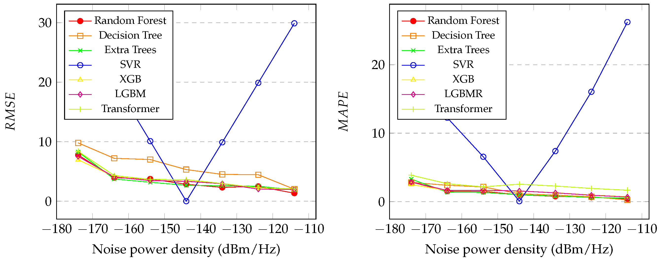
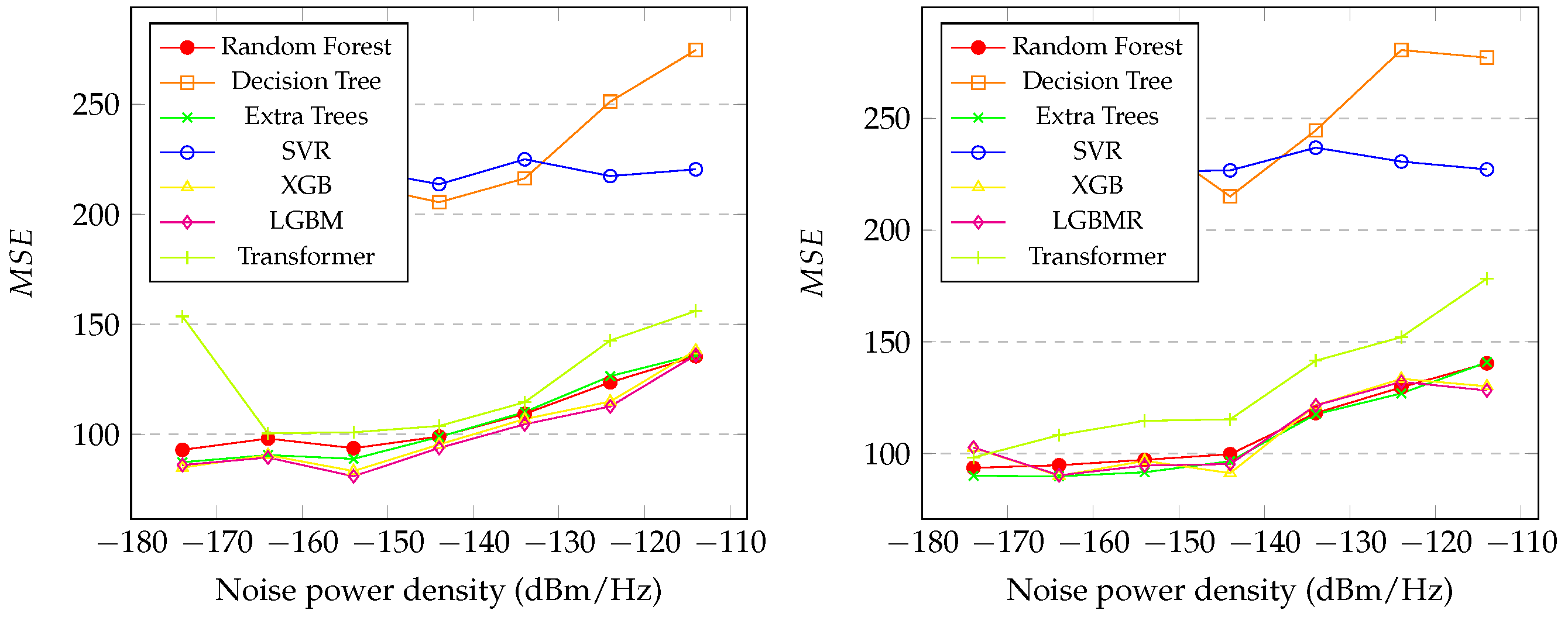
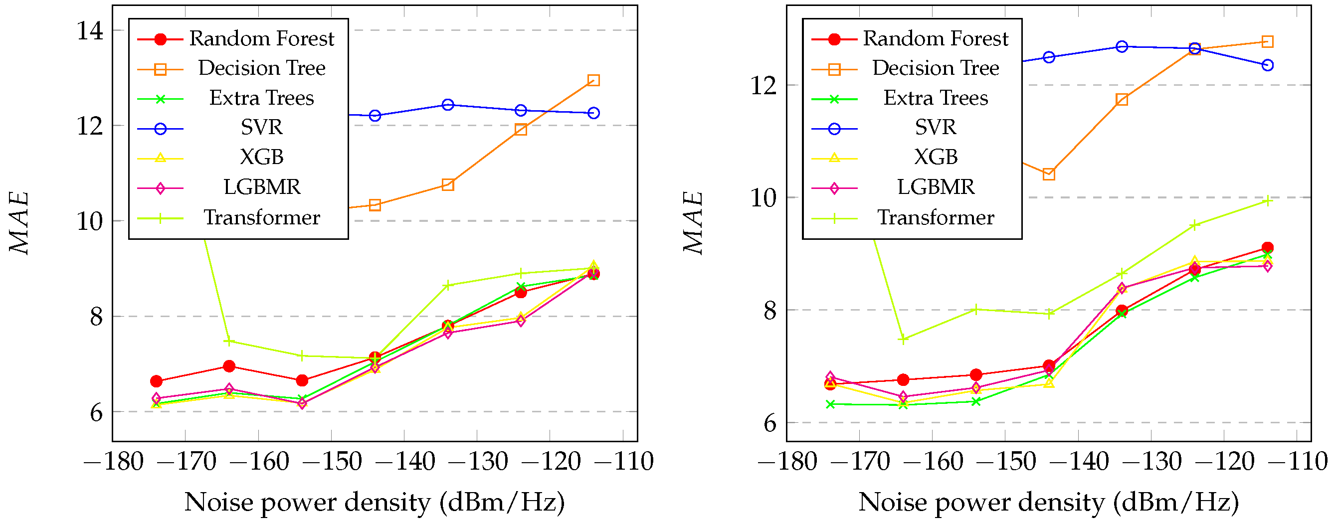
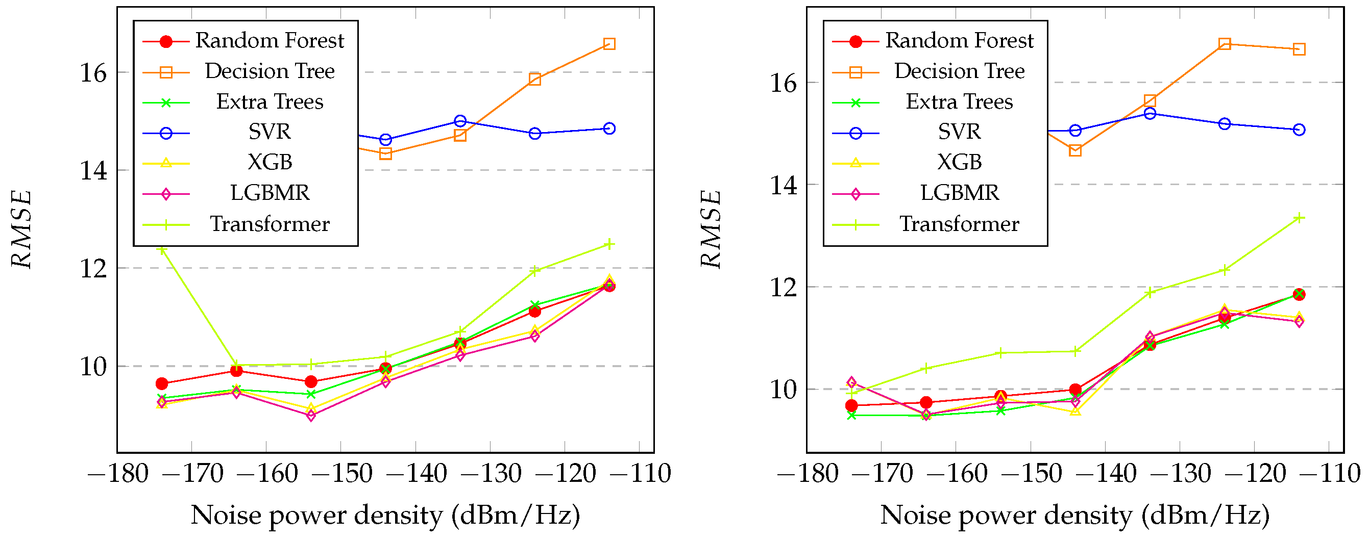
In Section 4.3, the results for noise prediction were presented, and several important aspects need to be highlighted. In Figure 3 (left), it is noticeable that the models achieved similar performance, except for decision tree and SVR. Interestingly, the best performance occurred at the highest levels of noise, except for SVR, which specialized in a single noise level, $-144$ dBm/Hz. Figure 3 (right) and Figure 4 (left and right) exhibit similar characteristics to Figure 3 (left). The overall results for random forest, XGB, LGBM, transformer, and extra trees are similar across all the metrics, with random forest and XGB performing particularly well, as demonstrated in Table 6. In contrast, SVR exhibited poor performance overall. Additionally, the correlation coefficients reveal that random forest, XGB, LGBM, and extra trees achieved strong correlations between the predicted and real noise values (Table 6). Due to the limited computational resources and the large amount of generated data, it was not possible to enhance the robustness of the transformer architectures. Furthermore, a search for optimal hyperparameter values for all the models could be a proposed enhancement for the work.

In Section 4.4, the results for the initial and final distance predictions were presented, and several notable observations arise. In Figure 5, it is evident that extra trees and LGBM achieved the highest performance. Unlike the noise prediction, the best performance for both distance predictions occurred at the lowest levels of noise for all the models, which was expected. The behavior of predicting the initial distance mirrors that of predicting the final distance, as indicated in Figure 5, Figure 6, Figure 7 and Figure 8. The general results for random forest, XGB, LGBM, transformer, and extra trees exhibit similarity across all the metrics, with extra trees, transformer, and LGBM slightly outperforming in almost all the metrics for both the initial and final distances, as shown in Table 7 and Table 8, respectively. In contrast, decision tree and SVR showed poor performance overall. Moreover, the correlation coefficients reveal that the predicted distances exhibited indices greater than $0.82$ in relation to the real values in both distances, initial and final. An interesting factor is that, in the initial distance prediction, the $MAPE$ values for the XGB and LGBM models returned ’inf’. More studies are needed to understand what happened.

6. Conclusions

In this paper, a noise and distance prediction method based on spectrum sensing signals using regression models was proposed. The conducted experiments have shown that the proposed methods hold promise for predicting noise levels, as well as the initial and final distances between the PU and SU. The correlation coefficient value for XGB is the highest and closest to one (Table 6), indicating a strong correlation between the predicted and actual noise values in the test database. As a result, the proposed methods can greatly benefit various applications, especially in telecommunication and networking, enabling the design of communication systems that meet appropriate requirements for ensuring reliable and efficient data transfer.

Additionally, the predictions for the initial and final distances between the PUs and SUs are presented as results. The conducted experiments have demonstrated that the proposed methods show promise in predicting distances between users. The correlation coefficient values for transformer are the highest, exceeding $0.82$ (Table 7 and Table 8), which implies a good level of correlation between the predicted distances and the actual distances in the test database. It is important to highlight that the number of possible noise levels is limited to seven ($-114$ to $-174$ dBm/Hz), while the number of possible distances is unknown since the distance was chosen randomly within a certain range of the area. Therefore, there may be a difference in performance between the two approaches. Hence, the proposed methods hold the potential to benefit numerous applications, including signal attenuation and path loss, interference and frequency reuse, fading and multipath effects, localization and tracking, and power control.

References

1. Valadão, M.D.; Amoedo, D.; Costa, A.; Carvalho, C.; Sabino, W. Deep cooperative spectrum sensing based on residual neural network using feature extraction and random forest classifier. Sensors 2021, 21, 7146. [Google Scholar] [CrossRef] [PubMed]
2. Lee, W.; Kim, M.; Cho, D.H. Deep cooperative sensing: Cooperative spectrum sensing based on convolutional neural networks. IEEE Trans. Veh. Technol. 2019, 68, 3005–3009. [Google Scholar] [CrossRef]
3. Valadäo, M.D.; Carvalho, C.B.; Júnior, W.S. Trends and challenges for the spectrum sensing in the next generation of communication systems. In Proceedings of the 2020 IEEE International Conference on Consumer Electronics-Taiwan (ICCE-Taiwan), Taoyuan, Taiwan, 28–30 September 2020; pp. 1–2. [Google Scholar] [CrossRef]
4. Valadão, M.D.; Amoedo, D.A.; Pereira, A.M.; Tavares, S.A.; Furtado, R.S.; Carvalho, C.B.; Da Costa, A.L.A.; Júnior, W.S. Cooperative spectrum sensing system using residual convolutional neural network. In Proceedings of the 2022 IEEE International Conference on Consumer Electronics (ICCE), Las Vegas, NV, USA, 7–9 January 2022; pp. 1–5. [Google Scholar] [CrossRef]
5. Valadão, M.D.; Júnior, W.S.; Carvalho, C.B. Trends and Challenges for the Spectrum Efficiency in NOMA and MIMO based Cognitive Radio in 5G Networks. In Proceedings of the 2021 IEEE International Conference on Consumer Electronics (ICCE), Las Vegas, NV, USA, 10–12 January 2021; pp. 1–4. [Google Scholar] [CrossRef]
6. Valadão, M.; Silva, L.; Serrão, M.; Guerreiro, W.; Furtado, V.; Freire, N.; Monteiro, G.; Craveiro, C. MobileNetV3-based Automatic Modulation Recognition for Low-Latency Spectrum Sensing. In Proceedings of the 2023 IEEE International Conference on Consumer Electronics (ICCE), Las Vegas, NV, USA, 6–8 January 2023; pp. 1–5. [Google Scholar] [CrossRef]
7. Gupta, M.S.; Kumar, K. Progression on spectrum sensing for cognitive radio networks: A survey, classification, challenges and future research issues. J. Netw. Comput. Appl. 2019, 143, 47–76. [Google Scholar] [CrossRef]
8. Arjoune, Y.; Kaabouch, N. A comprehensive survey on spectrum sensing in cognitive radio networks: Recent advances, new challenges, and future research directions. Sensors 2019, 19, 126. [Google Scholar] [CrossRef]
9. Shen, X.; Shi, D.; Peksi, S.; Gan, W.S. A multi-channel wireless active noise control headphone with coherence-based weight determination algorithm. J. Signal Process. Syst. 2022, 94, 811–819. [Google Scholar] [CrossRef]
10. Cheon, B.W.; Kim, N.H. AWGN Removal Using Modified Steering Kernel and Image Matching. Appl. Sci. 2022, 12, 11588. [Google Scholar] [CrossRef]
11. Ngo, T.; Kelley, B.; Rad, P. Deep learning based prediction of signal-to-noise ratio (SNR) for LTE and 5G systems. In Proceedings of the 2020 8th International Conference on Wireless Networks and Mobile Communications (WINCOM), Reims, France, 27–29 October 2020; pp. 1–6. [Google Scholar] [CrossRef]
12. Nagah Amr, M.; ELAttar, H.M.; Abd El Azeem, M.H.; El Badawy, H. An Enhanced Indoor Positioning Technique Based on a Novel Received Signal Strength Indicator Distance Prediction and Correction Model. Sensors 2021, 21, 719. [Google Scholar] [CrossRef]
13. Spüler, M.; Sarasola-Sanz, A.; Birbaumer, N.; Rosenstiel, W.; Ramos-Murguialday, A. Comparing metrics to evaluate performance of regression methods for decoding of neural signals. In Proceedings of the 2015 37th Annual International Conference of the IEEE Engineering in Medicine and Biology Society (EMBC), Milan, Italy, 25–29 August 2015; pp. 1083–1086. [Google Scholar] [CrossRef]
14. Jain, P.; Choudhury, A.; Dutta, P.; Kalita, K.; Barsocchi, P. Random forest regression-based machine learning model for accurate estimation of fluid flow in curved pipes. Processes 2021, 9, 2095. [Google Scholar] [CrossRef]
15. Wang, X.; Zhao, Y.; Pourpanah, F. Recent advances in deep learning. Int. J. Mach. Learn. Cybern. 2020, 11, 747–750. [Google Scholar] [CrossRef]
16. Su, X.; Li, J.; Hua, Z. Transformer-based regression network for pansharpening remote sensing images. IEEE Trans. Geosci. Remote Sens. 2022, 60, 5407423. [Google Scholar] [CrossRef]
17. Yao, G.; Hu, Z. SNR Estimation Method based on SRS and DINet. In Proceedings of the 2023 15th International Conference on Computer Modeling and Simulation, Dalian, China, 16–18 June 2023; pp. 218–224. [Google Scholar] [CrossRef]
18. Li, Y.; Bian, X.; Li, M. Denoising Generalization Performance of Channel Estimation in Multipath Time-Varying OFDM Systems. Sensors 2023, 23, 3102. [Google Scholar] [CrossRef] [PubMed]
19. Chatelier, B.; Corlay, V.; Ciochina, C.; Coly, F.; Guillet, J. Influence of Dataset Parameters on the Performance of Direct UE Positioning via Deep Learning. arXiv 2023, arXiv:2304.02308. [Google Scholar] [CrossRef]
20. Wang, C.; Xi, J.; Xia, C.; Xu, C.; Duan, Y. Indoor fingerprint positioning method based on real 5G signals. In Proceedings of the 2023 7th International Conference on Machine Learning and Soft Computing, Chongqing, China, 5–7 January 2023; pp. 205–210. [Google Scholar] [CrossRef]
21. Conti, A.; Morselli, F.; Liu, Z.; Bartoletti, S.; Mazuelas, S.; Lindsey, W.C.; Win, M.Z. Location awareness in beyond 5G networks. IEEE Commun. Mag. 2021, 59, 22–27. [Google Scholar] [CrossRef]
22. Yang, H.; Xie, X.; Kadoch, M. Machine learning techniques and a case study for intelligent wireless networks. IEEE Netw. 2020, 34, 208–215. [Google Scholar] [CrossRef]
23. Arjoune, Y.; Kaabouch, N. On spectrum sensing, a machine learning method for cognitive radio systems. In Proceedings of the 2019 IEEE International Conference on Electro Information Technology (EIT), Brookings, SD, USA, 20–22 May 2019; pp. 333–338. [Google Scholar] [CrossRef]
24. Chicco, D.; Warrens, M.J.; Jurman, G. The coefficient of determination R-squared is more informative than SMAPE, MAE, MAPE, MSE and RMSE in regression analysis evaluation. PeerJ Comput. Sci. 2021, 7, e623. [Google Scholar] [CrossRef]
25. Cichoń, K.; Kliks, A.; Bogucka, H. Energy-efficient cooperative spectrum sensing: A survey. IEEE Commun. Surv. Tutor. 2016, 18, 1861–1886. [Google Scholar] [CrossRef]
26. Segal, M.R. Machine Learning Benchmarks and Random Forest Regression; UCSF: Center for Bioinformatics and Molecular Biostatistics: San Francisco, CA, USA, 2004; Available online: https://escholarship.org/uc/item/35x3v9t4 (accessed on 18 March 2025).
27. Luo, H.; Cheng, F.; Yu, H.; Yi, Y. SDTR: Soft decision tree regressor for tabular data. IEEE Access 2021, 9, 55999–56011. [Google Scholar] [CrossRef]
28. Ahmad, M.W.; Reynolds, J.; Rezgui, Y. Predictive modelling for solar thermal energy systems: A comparison of support vector regression, random forest, extra trees and regression trees. J. Clean. Prod. 2018, 203, 810–821. [Google Scholar] [CrossRef]
29. Geurts, P.; Ernst, D.; Wehenkel, L. Extremely randomized trees. Mach. Learn. 2006, 63, 3–42. [Google Scholar] [CrossRef]
30. Zhang, X.; Yan, C.; Gao, C.; Malin, B.A.; Chen, Y. Predicting missing values in medical data via XGBoost regression. J. Healthc. Inform. Res. 2020, 4, 383–394. [Google Scholar] [CrossRef]
31. Chen, T.; Guestrin, C. Xgboost: A scalable tree boosting system. In Proceedings of the 22nd ACM SIGKDD International Conference on Knowledge Discovery and Data Mining, San Francisco, CA, USA, 13–17 August 2016; pp. 785–794. [Google Scholar] [CrossRef]
32. Ke, G.; Meng, Q.; Finley, T.; Wang, T.; Chen, W.; Ma, W.; Ye, Q.; Liu, T.Y. Lightgbm: A highly efficient gradient boosting decision tree. Adv. Neural Inf. Process. Syst. 2017, 30, 3146–3154. [Google Scholar]
33. Smola, A.J.; Schölkopf, B. A tutorial on support vector regression. Stat. Comput. 2004, 14, 199–222. [Google Scholar] [CrossRef]
34. Min, E.; Chen, R.; Bian, Y.; Xu, T.; Zhao, K.; Huang, W.; Zhao, P.; Huang, J.; Ananiadou, S.; Rong, Y. Transformer for graphs: An overview from architecture perspective. arXiv 2022, arXiv:2202.08455. [Google Scholar] [CrossRef]
35. Botchkarev, A. Evaluating performance of regression machine learning models using multiple error metrics in azure machine learning studio. SSRN Electron.J. 2018, 3177507. [Google Scholar] [CrossRef]
36. Benesty, J.; Chen, J.; Huang, Y.; Cohen, I. Pearson correlation coefficient. In Noise Reduction in Speech Processing; Springer: Berlin/Heidelberg, Germany, 2009; pp. 1–4. [Google Scholar] [CrossRef]
Figure 1. User position over time (initial state on the left; final state on the right).
Applsci 15 04296 g001
Figure 2. Architecture of the proposed transformer.
Applsci 15 04296 g002
Figure 3. Graphic of the M S E (left) and M A E (right) of proposed methods with N 0 between 114 dBm/Hz and 174 dBm/Hz.
Applsci 15 04296 g003
Figure 4. Graphic of the R M S E (left) and M A P E (right) of the proposed methods with N 0 between 114 dBm/Hz and 174 dBm/Hz.
Applsci 15 04296 g004
Figure 5. Graphic of the M S E (initial distance on the left and final distance on the right) of the proposed methods with N 0 between 114 dBm/Hz and 174 dBm/Hz.
Applsci 15 04296 g005
Figure 6. Graphic of the M A E (initial distance on the left and final distance on the right) of the proposed methods with N 0 between 114 dBm/Hz and 174 dBm/Hz.
Applsci 15 04296 g006
Figure 7. Graphic of the R M S E (initial distance on the left and final distance on the right) of the proposed methods with N 0 between 114 dBm/Hz and 174 dBm/Hz.
Applsci 15 04296 g007
Figure 8. Graphic of the M A P E (initial distance on the left and final distance on the right) of the proposed methods with N 0 between 114 dBm/Hz and 174 dBm/Hz.
Applsci 15 04296 g008