1. Introduction
This work builds upon our previous research [
1] presented at the SOCO 2024 Conference, where we introduced an initial methodology for HVAC temperature modeling. In this expanded study, we refine our approach by incorporating additional experimental validation, providing a more detailed performance analysis and enhancing the core of this study, which is the proper definition of a feature selection and extraction methodology. The improvements presented here aim to further optimize energy efficiency and predictive accuracy in HVAC systems.
In developed countries, buildings are responsible for an estimated 20–40% of total energy consumption with half of it being dedicated to maintaining thermal comfort [
2]. HVAC systems encompasses all the devices related to the management and regulation of temperature, humidity, and air quality within enclosed spaces. More adaptive and flexible HVAC systems have been shown to achieve energy savings ranging from 12.4 and 17.4% [
3] to as high as 25–32% [
4], within the established indoor comfort conditions. Many studies have successfully attempted to improve energy efficiency in HVAC systems [
3,
4,
5,
6,
7,
8], which goes hand-in-hand with proper thermal modeling of the studied system [
4,
9,
10,
11,
12,
13,
14,
15,
16,
17]. Similar approaches have been explored for optimizing the energy consumption of wireless sensor networks, applying ultra-low power techniques and energy harvesting to enhance efficiency and prolong operational lifespan [
18]. Numerous algorithms and software are used, and it is essential to decide which one to use to obtain a useful and accurate outcome with each system.
This work proposes a novel preprocessing methodology grounded in expert knowledge for feature selection and extraction, specifically designed to enhance the predictive accuracy of temperature and energy consumption of HVAC data-driven models. The proposed approach is based on studying the thermodynamic interactions that describe the system to accordingly select the variables that have a meaningful impact on the studied system and creating dynamic variables that can contain information from multiple features to reduce the space of inputs of the data-driven model. The significance of this approach lies in understanding the thermodynamic interactions and the physical equations that describe these interactions, thereby exploring innovative criteria for feature selection and creation. Notably, the contributions of this paper include the utilization of real data from a non-residential building, providing a robust basis for model validation. Furthermore, the case study focuses on a complex HVAC system featuring a fan coil that extracts energy from an inertia tank. This unique setup underscores the general applicability of the proposed methodology, demonstrating its potential to address advanced HVAC configurations and improve predictive accuracy in various real-world applications.
The rest of this work is organized as follows:
Section 2 outlines the three primary families of HVAC modeling approaches and introduces support vector regression.
Section 3 reviews the state-of-the-art in HVAC systems and data preprocessing techniques.
Section 4 details the methodology, elaborating on the novel contributions to ensure reproducibility.
Section 5 describes the building, the HVAC system used, its operational characteristics, and the application of the proposed methodology.
Section 6 presents simulation results and analyzes the model’s performance. The work concludes with a summary of key findings and suggestions for future research directions in
Section 7.
2. Background
Reliable temperature forecasting in HVAC systems is essential for improving energy efficiency and indoor comfort. Common modeling techniques are classified as either data-driven, physics-based, or hybrid, and each offer advantages and limitations. This chapter reviews these approaches and introduces the SVR modeling technique, which is applied in later sections.
2.1. HVAC Modeling Techniques
There are different methods to tackle the thermal approach of a system and each can be linear or nonlinear, static or dynamic, explicit or implicit, discrete or continuous, deterministic or probabilistic, deductive, inductive or floating [
19]. Different methodologies have been employed in numerous studies to tackle the thermal problem. However, it is essential to identify which method most accurately predicts the system’s behavior to enable proper optimization.
2.1.1. Physics-Based Models
Physics-based models are constructed on the foundational principles of thermodynamics, such as Fourier’s law of thermal conduction and the Navier–Stokes equations, among other energy and mass balance equations. While these models can yield high accuracy by solving the equations analytically, this approach is often impractical due to the complexity and time-consuming nature of numerically solving the coupled partial differential equations. Additionally, an in-depth understanding of the system is essential; otherwise, numerous assumptions must be made, which can lead to discrepancies between the computed results and real-world observations. Numerous studies have focused on various components of HVAC systems. Browne and Bansal [
20] employed a thermal capacitance approach to predict chiller performance, achieving results within ±10%. Lei and Zaheereuddin [
21] utilized mass and energy balance techniques to analyze the transient response of refrigeration systems. In the context of thermal zones, Ghiaus and Hazyuk [
22] applied heat equations to dynamically simulate heating loads, while Goyal et al. [
23] used an RC network model to predict zone temperatures, accounting for heat losses through walls. These studies highlight the importance of selecting appropriate methodologies to accurately predict and optimize HVAC system performance.
2.1.2. Data-Driven Models
Data-driven models leverage empirical data and employ machine learning techniques such as artificial neural networks, fuzzy networks, and genetic algorithms to establish relationships between features and target variables. These approaches are highly dependent on the quality and quantity of the available training data and can account for disturbances in the data, such as variability in occupancy, the usage of electronic devices, and other environmental factors. However, they capture the physics of the process to a minimal extent. Wei et al. [
3] successfully integrated an MLP with MOPS framework, achieving energy savings of 12.4–17.4%. Similarly, Kusiak et al. [
5] applied a multi-objective optimization model in combination with an evolutionary computation algorithm, resulting in energy savings of 21.4–22.6%. Additionally, Huang et al. [
7] utilized an ANN model to capture thermal interactions in multi-zone buildings, demonstrating that comfortable temperatures can be maintained with a 28% reduction in daily energy consumption and an estimated 10% savings when the model is extended over a month.
2.1.3. Hybrid Models
Hybrid models represent an advanced synthesis of data-driven and physics-based methodologies. These models are grounded in physical laws, while their parameters are estimated using data-driven techniques derived from experimentally obtained training data. Such models excel in scenarios where the studied system encompasses physical interactions that are not explicitly defined and where the training dataset is relatively sparse. This dual approach enables hybrid models to effectively capture the complexities of the system, thereby enhancing the accuracy of predictions and overall system optimization. Afram and Janabi-Sharifi [
24] derived the energy balance equations for each HVAC subsystem and estimated the parameters utilizing the nonlinear least squares optimization technique, successfully capturing the impact of ON/OFF controllers on energy consumption with high accuracy. Similarly, Rao and Ukil [
15] employed numerically simulated temperature data to estimate the parameters of a semi-nonlinear thermal model designed to approximate the temperature dynamics of a room, using FloVENT software version 9.3. Additionally, Wu and Sun [
16] developed a physics-based Auto-Regressive Moving Average with Exogenous Inputs (pbARMAX) model to predict room temperature, demonstrating a root mean squared error of less than 0.10 over a four-week period.
2.2. Support Vector Regression
SVR was first introduced by Vapnik [
25] as a method for estimating regressions and approximating functions as a generalization of their previous work support vector machines [
26]. Support vector regression operates by finding the optimal hyperplane that best fits the training data while maximizing the margin between data points. The key components of SVR include kernel functions to map input data into high-dimensional feature spaces; epsilon (
) and regularization (
C) parameters as hyperparameters to control the model’s behavior with epsilon as the margin width within which data points are considered correctly predicted, while
C balances the trade-off between achieving a small margin and minimizing training error; and support vectors as points lying exactly on the margin or within it, which heavily influence the construction of the regression model.
This modeling technique offers several advantages that make it a valuable tool in data modeling. It performs effectively in high-dimensional spaces, is memory-efficient, and demonstrates robustness against overfitting. Additionally, SVR excels at modeling complex, non-linear relationships. However, it also has certain limitations, including computational complexity when dealing with large datasets as its computational cost scales between
and
[
27], sensitivity to hyperparameter tuning, and challenges in handling noisy data. Despite these drawbacks, it has been successfully applied in various fields such as financial forecasting, environmental modeling and bioinformatics [
28]. As a powerful regression technique, SVR remains relevant even in the deep learning era, providing a mathematically sound approach for capturing intricate patterns within data.
3. State of the Art
This chapter provides a review of the current advancements in HVAC system modeling and data preprocessing techniques. The first section delves into the latest data preprocessing techniques specific to HVAC modeling, highlighting methods for data cleaning, feature selection, and transformation that enhance model performance and reliability. The second section explores the state-of-the-art in HVAC modeling methodologies, examining recent developments across data-driven, physics-based, and hybid modeling approaches and their applications in improving forecasting accuracy and efficiency.
3.1. Data Preprocessing Techniques
Preprocessing data before using it for HVAC model training is essential due to the inherent complexity and variability of the system data, which are typically composed of time-series sensor information. Proper preprocessing improves data quality, facilitates feature extraction, and enhances the model’s ability to detect patterns. Key preprocessing techniques used in HVAC modeling are reviewed here.
The presence of missing data in HVAC systems can result from sensor failures or communication issues. Several techniques exist for dealing with missing values, each varying in complexity and suitability depending on the nature of the data. Common methods for handling missing data include mean or median imputation, where missing values are replaced by the central tendency of the available data. For more sophisticated imputation, techniques such as kNN [
29] or MICE [
30,
31] are employed, which consider the correlations between variables to fill in missing values more accurately.
Outliers in HVAC data can significantly affect the performance of predictive models. Various methods, such as Z-score and IQR, are used to detect and remove data points that deviate from the expected range. More advanced methods like IF [
32] or LOF [
33] are also utilized to handle outliers in large datasets where traditional methods may be less effective.
HVAC data is often noisy due to fluctuations in sensor readings. Smoothing techniques, such as Gaussian filtering [
34] or moving averages, are applied to time-series data to reduce noise and reveal underlying trends. This enhances model accuracy by providing cleaner features.
Data normalization is essential to ensure that different features have comparable scales, preventing any single feature from disproportionately influencing model results. Common techniques include Min-Max scaling and standardization.
High-dimensional HVAC datasets, particularly those with many sensors or features, may suffer from issues such as overfitting and computational inefficiency. PCA [
35] is commonly used for dimensionality reduction, helping to retain the most significant features while discarding less informative ones. t-SNE [
36] and UMAP [
37] are also employed for visualizing high-dimensional HVAC data, though they are less commonly used for direct model training.
Preprocessing is a standard practice in machine learning; the following are examples of papers that apply a variety of the explained techniques. Richter and Abida [
38] applied data cleaning and normalization for neural network control, while Tang et al. [
39] used clustering for short-term temperature and CO
2 predictions. Advanced methods, including weight clustering (Wang et al. [
40]) and LSTM-based interpolation (Mtibaa et al. [
41]) improve load predictions and multistep forecasting. Xiao et al. (2022) [
42] are the first authors to investigate the influence of data preprocessing and selection on the accuracy of HVAC energy consumption models. Their study emphasizes common preprocessing practices such as data imputation, resolution processing, normalization, outlier detection, and smoothing. Despite this contribution, the role of preprocessing, feature selection, and extraction remains underexplored. This work seeks to address this gap by establishing a methodology to identify key variables and define new ones based on expert knowledge and physics equations. By reducing the dimensionality of features used in data-driven models, the objective is to simplify the process while enhancing the accuracy of temperature and energy consumption forecasts for HVAC systems.
3.2. HVAC Modeling Approaches
As seen in
Section 2.1, HVAC modeling approaches can be categorized into physics based, data-driven, and hybrid models, each with its own strengths and weaknesses.
Physics-based models excel in generalization but have low prediction accuracy, and while they require little data, they are complex. Data-driven models can vary widely in both prediction accuracy and generalization but are simpler and data-intensive. Hybrid models strike a balance with high prediction accuracy, medium generalization, and moderate complexity and data requirements [
19].
Table 1 encapsulates the trade-offs and considerations for choosing between different modeling techniques in various applications, highlighting their strengths and weaknesses.
Hybrid models have gained popularity due to their ability to combine the strengths of both physics-based and data-driven approaches. These models offer improved prediction accuracy, adaptability, and leverage physics-based simulations while addressing some of the limitations of purely data-driven or physics-based models [
43]. At the same time, data-driven approaches, particularly those utilizing machine learning and artificial intelligence, have seen significant advancements. These methods offer high adaptability and efficiency in cost-saving, with promising performance compared to other approaches [
19].
Modeling HVAC systems presents significant challenges due to their non-linear, dynamic, and multi-variable nature, making purely physics-based models difficult to implement effectively. Classical approaches rely on solving complex differential equations that require detailed knowledge of system parameters and are computationally intensive, making real-time applications impractical. Furthermore, HVAC performance is influenced by external factors like occupant behavior, weather conditions, and sensor variability, which are difficult to represent accurately with fixed physical models. In contrast, a data-driven framework leverages historical and real-time sensor data to automatically capture complex relationships between temperature dynamics, energy consumption, and external conditions without the need for explicit equations.
Machine learning techniques excel in handling non-linear dependencies, allowing for improved forecasting accuracy and adaptability to changing conditions. Additionally, data-driven models require less computational power after training, enabling faster predictions compared to iterative numerical solutions of physical equations. Another advantage is scalability, as physics-based models must be redefined for each specific HVAC system, while machine learning models can generalize across different buildings by training on diverse datasets. For these reasons, a data-driven approach was chosen as it provides a more flexible, accurate, and computationally efficient solution for HVAC modeling and forecasting.
4. Methodology
This section outlines the novel preprocessing methodology based on expert knowledge for modeling HVAC system dynamics. The approach is designed for applicability to similar energy-efficient HVAC systems using data-driven models, with this new preprocessing method aimed at reducing and simplifying the dataset provided to the model.
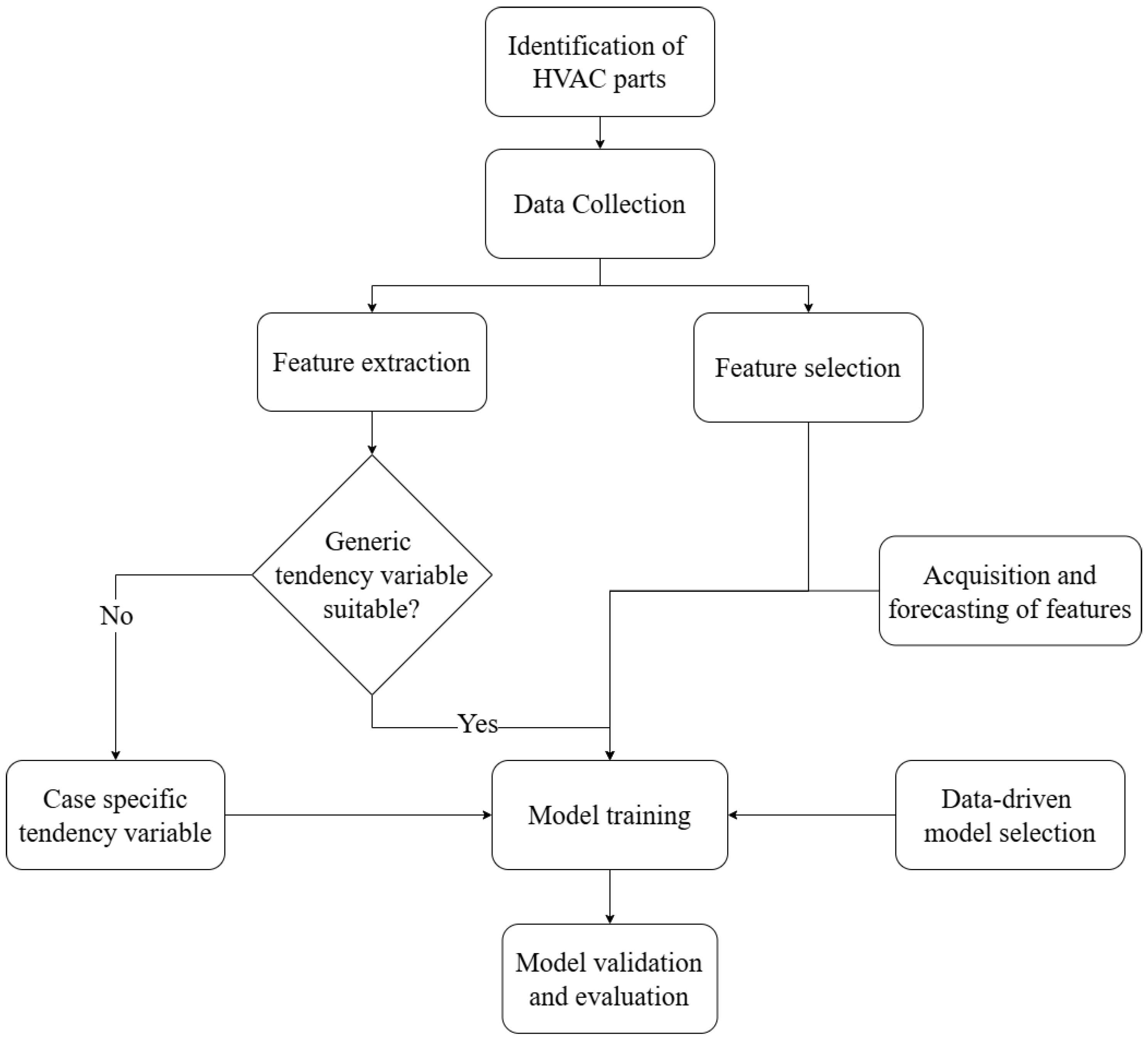
Notably, the methodology is designed to be applied to a recursive modeling strategy, where the model predicts a step in the future and utilizes its previous predictions to inform subsequent forecasts. A block diagram illustrating the complete process of modeling an HVAC system is presented in
Figure 1.
The methodology is composed of seven steps to model the temperature profile of a acclimatized room that uses an HVAC system:
Analysis of the studied case: identification of key components of the HVAC system (e.g., energy storage device).
Data collection: raw data are gathered from the system’s sensors, including temperature, humidity, energy consumption, and occupancy levels.
Feature selection and extraction: key features are selected and new ones are defined based on expert knowledge and thermodynamic principles to accurately capture the system’s dynamics.
Acquisition and forecasting of essential features required at each time instant to ensure the model’s completeness.
Model selection: a proper data-driven model is chosen to handle the non-linearities of the thermal system.
Model training: the model is trained using historical data from the system, tuning hyperparameters to optimize performance.
Model validation and evaluation: the trained model is validated using a separate test dataset, and performance is measured using R2 and MAPE metrics.
Step 1 focuses on thoroughly understanding the HVAC system under study. This involves identifying the critical components within the system, such as the energy storage device, heat exchangers, ventilation units, and other key equipment. Understanding the role of each component in the system helps establish a clear picture of the factors influencing the HVAC system’s performance and energy dynamics. This analysis serves as the foundation for subsequent steps, ensuring that all relevant elements are considered when building the predictive model.
Step 2 is to gather raw data from the system’s sensors. The primary variables collected include temperature, humidity, energy consumption, and room occupancy, which all play significant roles in HVAC system behavior. These data often come from distributed sensors within different zones of a building, capturing a wide range of conditions. By collecting comprehensive data, it is ensured that the full spectrum of variables affecting the system is captured. Data quality and consistency are key here, as inaccuracies or gaps in data can adversely affect model performance.
The critical contribution of this work lies in step 3, feature selection and extraction, which follows a specific format and introduces a novel approach to define key variables. This step transforms standard modeling practices by incorporating thermodynamic principles into the selection and creation of variables. This step is explained in detail in
Section 4.2 and
Section 4.3.
In step 4, essential features, identified as critical to each time instant of the modeling process, are either acquired or forecast as needed. This step ensures that all relevant features are available at every stage, supporting the model’s completeness and accuracy. Forecasting may be employed when future values of certain variables (e.g., expected occupancy levels or outdoor temperatures) are required for predictions but are not directly measured in real-time. This step is explained in detail in
Section 4.1.
A suitable model is chosen in step 5 to account for the inherent complexities of the HVAC system, including its non-linear behaviors. A data-driven modeling approach is often appropriate here, allowing the model to capture complex relationships within the data. Selecting an appropriate model architecture is key to balancing predictive power with computational efficiency, ensuring the model can handle the HVAC system’s unique characteristics.
In step 6, the chosen model is trained on historical data gathered from the HVAC system. During this process, the model learns patterns and relationships within the data, fine-tuning its parameters to improve its predictive accuracy. Hyperparameters are carefully adjusted to optimize the model’s performance without overfitting. Training the model on a large and representative dataset allows it to generalize well to new data, making it robust for future predictions. This step may also involve regularization techniques to prevent overfitting, enhancing the model’s generalizability.
Finally, in step 7, the trained model is validated using a separate test dataset, distinct from the training data, to evaluate its real-world predictive performance. Validation metrics such as the coefficient of determination (R2) and the mean absolute percentage error (MAPE) are used to assess the model’s accuracy and reliability. This step provides insights into the model’s strengths and potential limitations, ensuring it meets the required performance standards before deployment.
The proposed methodology focuses on a recursive model structure, where the model uses its past outputs as inputs for future predictions as seen in
Figure 2. This approach inherently involves feeding the forecast values back into the model at each time instant, creating a sequence of predictions over time. Consequently, error accumulation is expected, as small inaccuracies in early predictions can propagate and amplify throughout the forecasting process. Additionally, any external variables or factors not forecast by the model must be known at each time instant to ensure accurate predictions and maintain consistency within the recursive framework.
4.1. Features Acquisition and Forecasting
The methodology is designed for a model to perform iterative forecasting, so it is critical to have all the features that significantly affect the model available at each time instant. For example, exterior temperature is a key feature in any HVAC system; its value can be continuously monitored or forecast using data from weather APIs. Room occupancy is another crucial feature, as it significantly impacts indoor temperature. However, predicting occupancy is challenging due to the variability in human behavior.
Nevertheless, approximations can be made based on factors like work schedules if the room is a workspace. When schedules are unavailable but a sensor provides real-time occupancy data, modeling this occupancy over time can be achieved using techniques such as autoregressive models, moving averages, or machine learning algorithms. These approaches help capture occupancy trends, supporting more accurate and dynamic HVAC forecasting even when human patterns are unpredictable. Furthermore, a simple approach is to approximate the values as a Gaussian function:
where
. Using the
curve_fit function from the
scipy.optimize library [
46], this Gaussian function, along with any other appropriate function, can be fitted to the observed occupancy data to estimate the number of people in the room based on past trends. This approach offers a smooth approximation of occupancy variations over time.
4.2. Feature Selection
Feature selection is important to obtain a model that can capture precisely the dynamics of an HVAC system. Data-driven models rely heavily on data to identify patterns and make predictions; however, generally, it is almost impossible to interpret their decision-making process. Modeling an HVAC system is fundamentally a thermodynamics problem, necessitating that the model resemble the behavior of heat transfer equations. To guide the model in understanding the processes occurring within the system, the thermal interactions are first described to facilitate proper feature selection. The focus is on detailing which thermal interactions occur and then choosing features that represent or significantly impact the system based on their similarity to variables in thermodynamic equations.
According to thermodynamics, heat transfer can take place in the form of conduction, convection, or radiation. Radiation involves the emission of electromagnetic waves by all objects at temperatures above absolute zero. However, radiation loss becomes significant only at high temperatures. Considering a typical HVAC temperature range of 8 °C to 50 °C, this interaction can be neglected.
Convection, the transfer of energy through fluid movement, significantly impacts room temperature, as hot air circulated by a fan coil heats the entire space. The objective is not to predict the temperature at every point in the room, but rather to establish a single representative temperature for each HVAC element. Consequently, detailed spatial temperature predictions are not considered in this process.
Conduction is the process by which heat is transferred from a region of higher temperature to a region of lower temperature within an object. HVAC systems typically focus on interactions involving fluids, such as air and water, rather than solid objects. To simplify the analysis, the system can be modeled by considering the HVAC unit and the acclimatized room as contiguous blocks, with the exterior environment acting as a third block. In this context, thermal interactions are governed exclusively by conduction. Analyzing Newton’s law of cooling (Equation (
2)) provides valuable insights into the importance of the variables involved:
Here,
q represents the heat flux transferred into or out of the body,
h denotes the heat transfer coefficient, and
signifies the temperature difference between the two objects. This equation highlights the importance of the heat sources and the temperatures of the interacting objects.
Based on this information, a study must be conducted for each case to identify the heat sources that significantly impact the temperature system (e.g., the number of people, operating electrical devices, server racks, etc).
4.3. Feature Extraction
The emphasis here is on minimizing and simplifying the data provided to the models to accurately represent the underlying thermodynamic processes to the machine learning model. This approach is aimed at improving the model’s performance and accuracy.
From Equation (
2),
, where
represents the temperature of the environment, which is the temperature toward which the system tends at any given moment. Consequently, a new variable called
tendency is defined. This variable aims to capture the temperature toward which the system’s temperature is expected to tend, taking into account the HVAC instructions and the current state of the system. To accurately define this new variable, it is necessary to understand the HVAC system’s logic and the conditions under which the HVAC should be activated or deactivated.
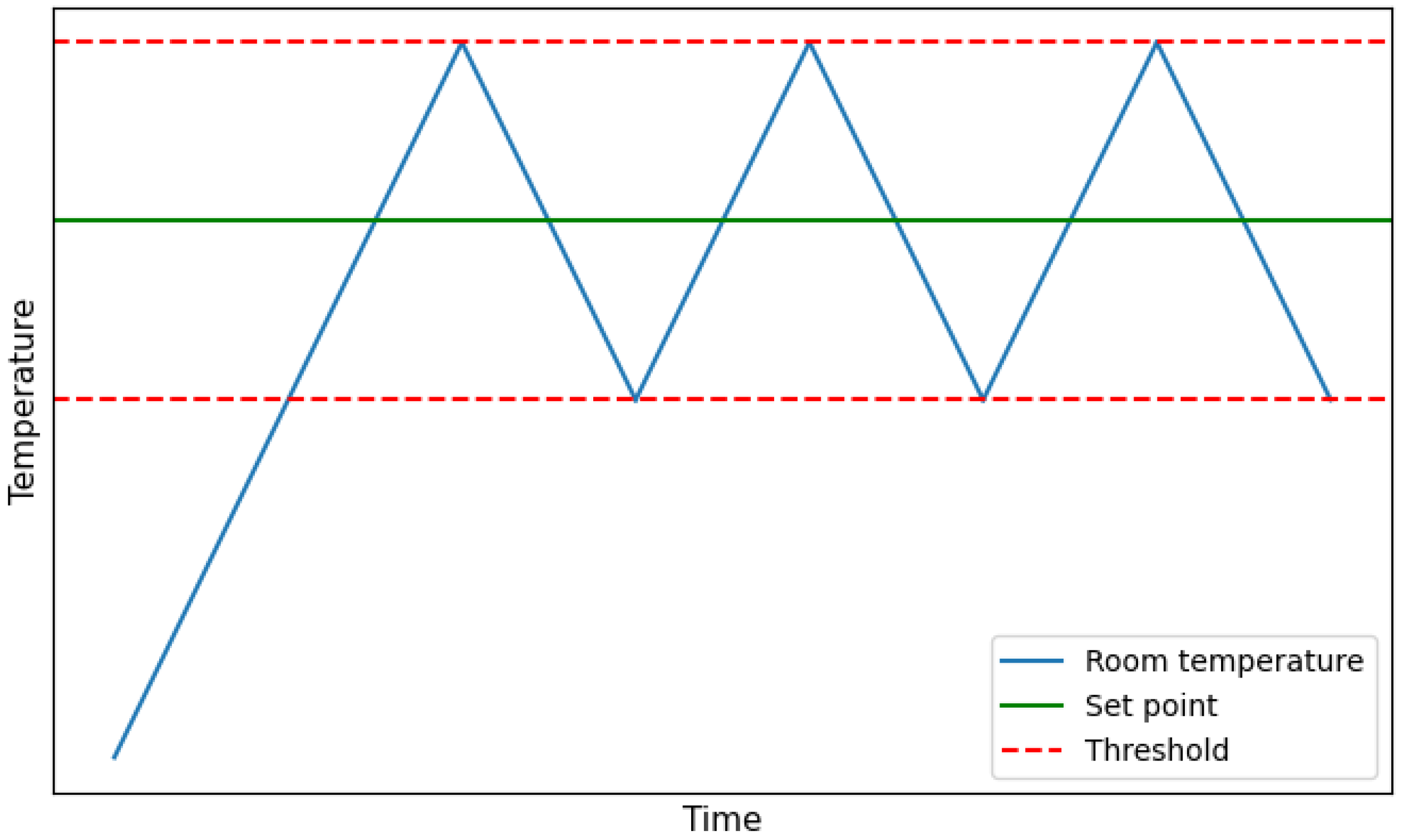
Typically, acclimatized rooms operate based on a straightforward rule: if the temperature drops below the set point, the HVAC system is activated, and if the temperature exceeds the set point, the HVAC system is deactivated. This rule is implemented with considerable precision, incorporating both an upper and a lower threshold. When heating the room, the system continues to heat until the temperature reaches the set point plus the upper threshold. Conversely, when the HVAC system is off, the room cools down until the temperature falls below the set point minus the lower threshold.
Figure 3 illustrates this oscillating state as the room is heated.
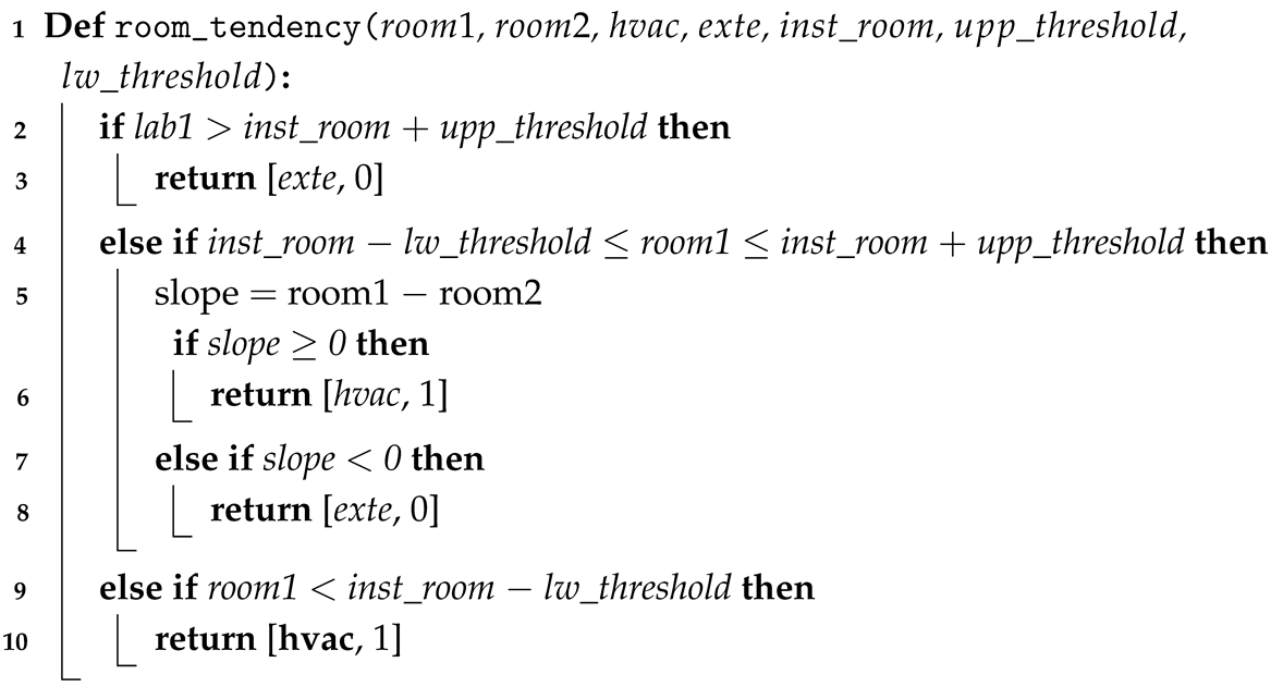
With each change in the direction of the oscillation, the room tends toward a specific temperature. When the room is being heated, it tends toward the temperature of the air pumped by the HVAC system. When it is cooling down, it tends toward the outdoor temperature. A challenge arises when the temperature is located between the thresholds: with only one point, it is impossible to determine whether the temperature should increase or decrease. To resolve this and determine the direction of the temperature, the closest previous point is examined, and the slope between them is calculated. A positive slope indicates that the room’s temperature will tend toward the air pumped by the HVAC, while a negative slope suggests it will tend toward the exterior temperature. Based on this understanding, the general Algorithm 1 is defined in the function
room_tendency.
| Algorithm 1: Temperature tendency of the room |
Input: room1: Temperature of the room at time t−1 room2: Temperature of the room at time t−2 hvac: Temperature of the air expulsed by the HVAC at time t−1 exte: Exterior temperature at time t inst_room: Instruction for the room at time t upp_threshold: Upper threshold lw_threshold: Lower threshold Output: Vector: [Tendency temperature, 1 fan coil is ON 0 if fan coil is OFF] |
![Applsci 15 04291 i001]() |
Algorithm 1 shows the general function that should follow the tendency temperature of a room, while also returning the HVAC status for energy consumption prediction. This serves as a universal formula but may need adjustments based on the specific requirements of each system. The computational cost of executing this function is .
The objective is to simplify the features provided to the model, ensuring alignment with those used in Equation (
2). Consequently, the final set of features for a generic one-room system with an air conditioner should include all relevant heat sources, the temperatures of adjacent spaces that significantly impact the target room (e.g., exterior temperature), and the temperature tendency.
5. Case Study
The HVAC system under study is installed in a workplace room at the University of Girona. This room is situated on the first floor of the P4 building of the Montilivi campus, surrounded by other working areas. It has an exterior wall with northwest-facing windows. The geometrical dimensions of the room are 9.83 m (length) × 7.25 m (width) × 3.00 m (height).
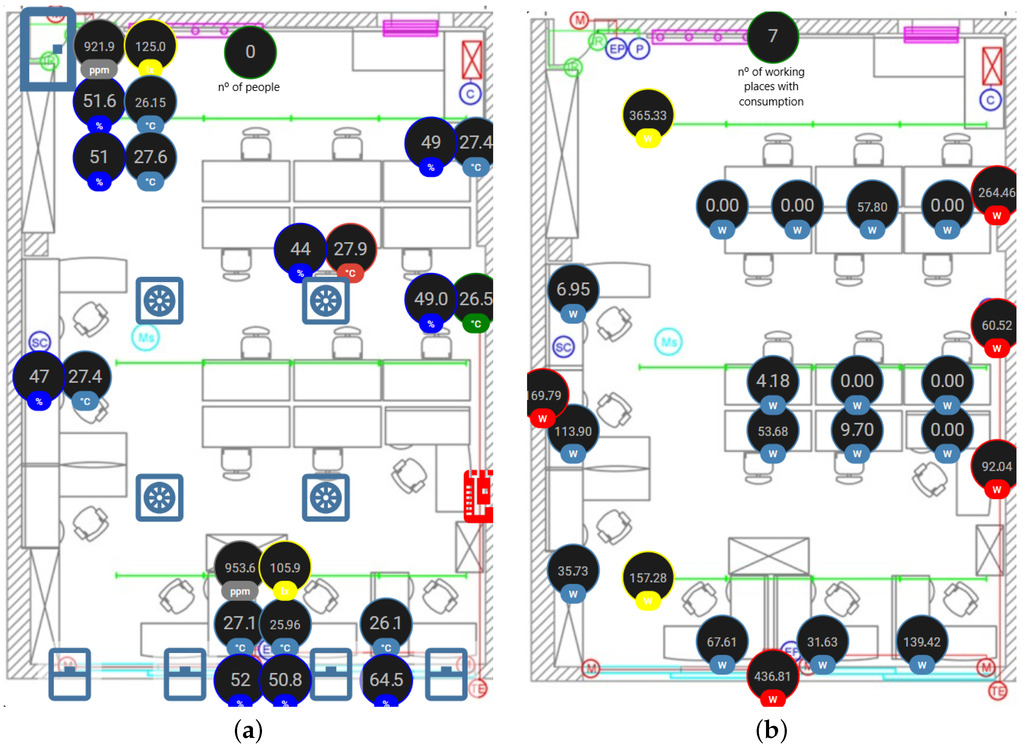
The room, hereafter referred to as the laboratory, is used daily by researchers as an office. It is equipped with numerous sensors for monitoring humidity, temperature, energy consumption and person zone by zone as displayed in
Figure 4a,b.
The HVAC system, depicted in
Figure 5, utilizes geothermal energy during winter mode, extracted from a 100-m-deep well with a stable temperature range of 15.0–17.0 °C. Water circulates to harness the geothermal energy, which then passes through a compression/expansion heat pump. The extracted energy is stored in an inertia tank and subsequently used by the fan coil to acclimatize the laboratory. This system is versatile, capable of providing both cooling in summer and heating in winter.
Figure 5 shows the four zones where data are collected. The first, in orange, is the laboratory or the acclimatized zone. The second, in light gray, is the machine room where the heat bomb and inertia tank are located, displaying its temperature. The light green zone is the exterior of the building where the temperature is collected. The last zone, in light orange, represents the well and its temperature at 100 m below ground.
Every sensor and controller is monitored through a web interface called the Control Assistant, designed by the university researchers. This platform manages all instructions for the HVAC system, from setting the temperature of the inertia tank and laboratory to controlling the opening and closing of windows. Each sensor collects real-time data, which are stored in a database. The data storage rate can be adjusted to the desired frequency; however, to avoid overloading the database, the default setting is to collect data every five minutes.
Within the Control Assistant, a set of target temperatures can be defined for both the laboratory and the inertia tank to maintain a comfortable indoor environment. These target temperatures should be adjusted according to seasonal variations in outdoor temperatures. Therefore, two modes are defined: summer mode and winter mode. Each mode sets specific temperature targets based on the time of day,
h.
5.1. Dataset Description
This paper focuses on the winter mode, from which all data were collected and used to build the models. The dataset extends from 2024-01-22 to 2024-04-29 with a granularity of 5 min. After removing all the instances with errors and missing values, the resulting dataframe contains 24,203 useful rows for each sensor described in the previous section. The collected dataset encompasses a wide range of temperatures. To ensure a comprehensive model, the dataset is randomly partitioned for testing by selecting 11 days, equivalent to 15% of the total data, as the test set, while the remaining data are used for training.
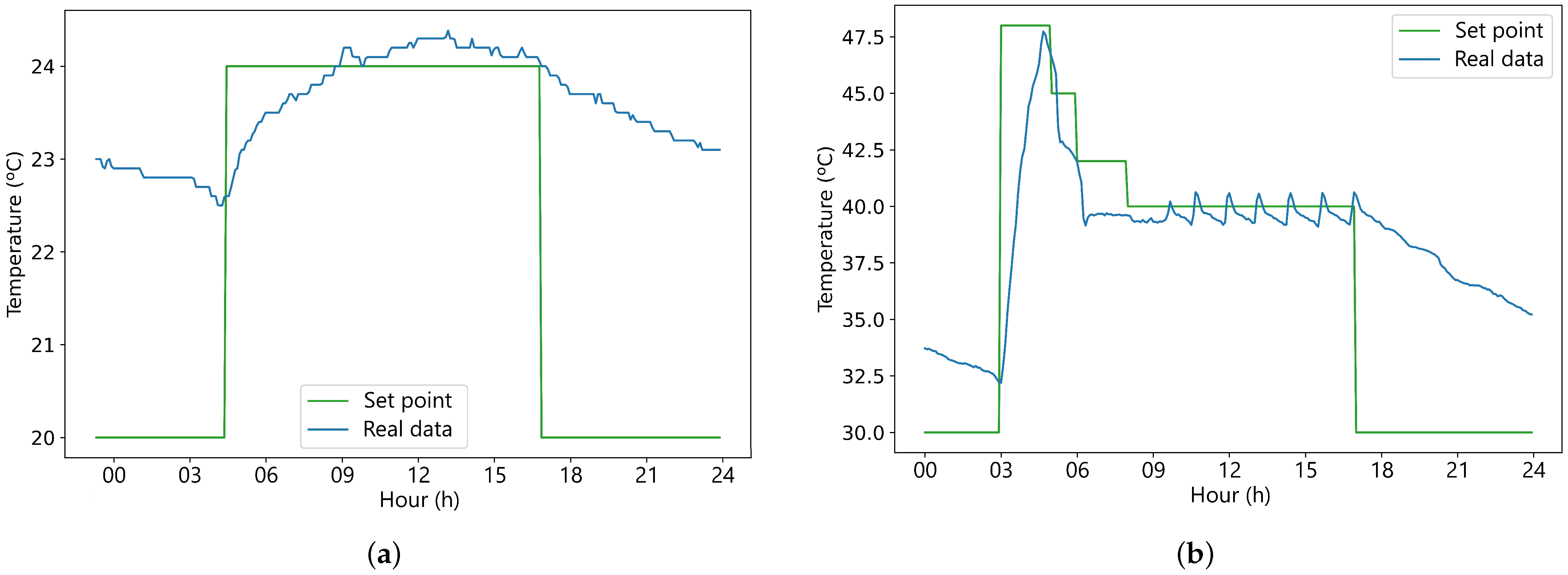
Figure 6a,b display an example of a complete day in winter mode of set points for the laboratory and inertia tank with its respective values of real temperature.
5.2. Feature Selection
Features are selected according to the methodology outlined in
Section 4.2, treating the inertia tank, the laboratory, and the exterior as three distinct blocks with varying temperatures in contact.
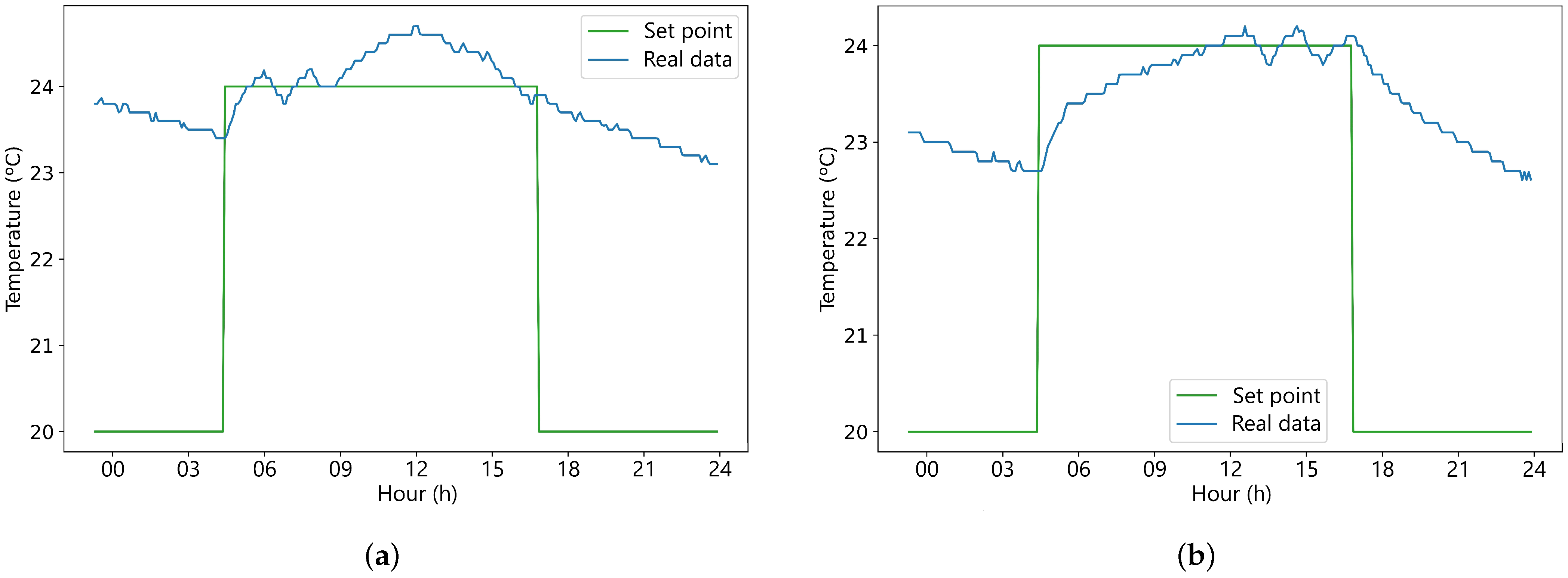
The first step is to identify heat sources, and a clear difference in temperature dynamics is observed between weekdays, when the laboratory is occupied with investigators working, and weekends when the laboratory is empty. As an example,
Figure 7a shows how during working hours, the temperature increases due to the presence of investigators, going above the set point; in contrast,
Figure 7b presents a more gradual approximation and stabilization around the set point on a weekend day when no-one entered the laboratory.
This observation highlights the number of people as a heat source with a substantial influence on the laboratory’s temperature.
Referring to Equation (
2), the temperature of the inertia tank, the outdoor temperature, and the number of people are identified as crucial features for predicting the laboratory’s temperature. These features have a significant impact on the system and will be used to train the laboratory’s model.
The features that affect the inertia tank are straightforward to identify since this element is more isolated than the laboratory. The heat flux of the inertia tank will be through the machine room, the laboratory if the fan coil is ON or OFF, and its own set point heating the tank when it gets below the target temperature.
Table 2 displays the features selected to build the models with their types and short descriptions.
Table 2 collects the features that describe the systems according to their thermodynamic properties and those will be the variables used to train the models. It is essential to note that the primary objective of the models is to predict the temperatures of both the laboratory and the inertia tank. Therefore, all features used to train the models must be available for each time instant at which a forecast is to be made in the future.
5.3. Feature Extraction
In this section, step 3 of the methodology is applied to the fan coil and inertia tank components. For the fan coil, the feature extraction process follows the same algorithm described in the methodology, ensuring consistency across the analysis. However, the inertia tank requires a customized function to accommodate its unique characteristics, while still adhering to the core principles of the methodology. This approach ensures methodological coherence while addressing the specific needs of each component.
5.3.1. Laboratory Tendency Temperature
The laboratory follows the exact same process as that described in
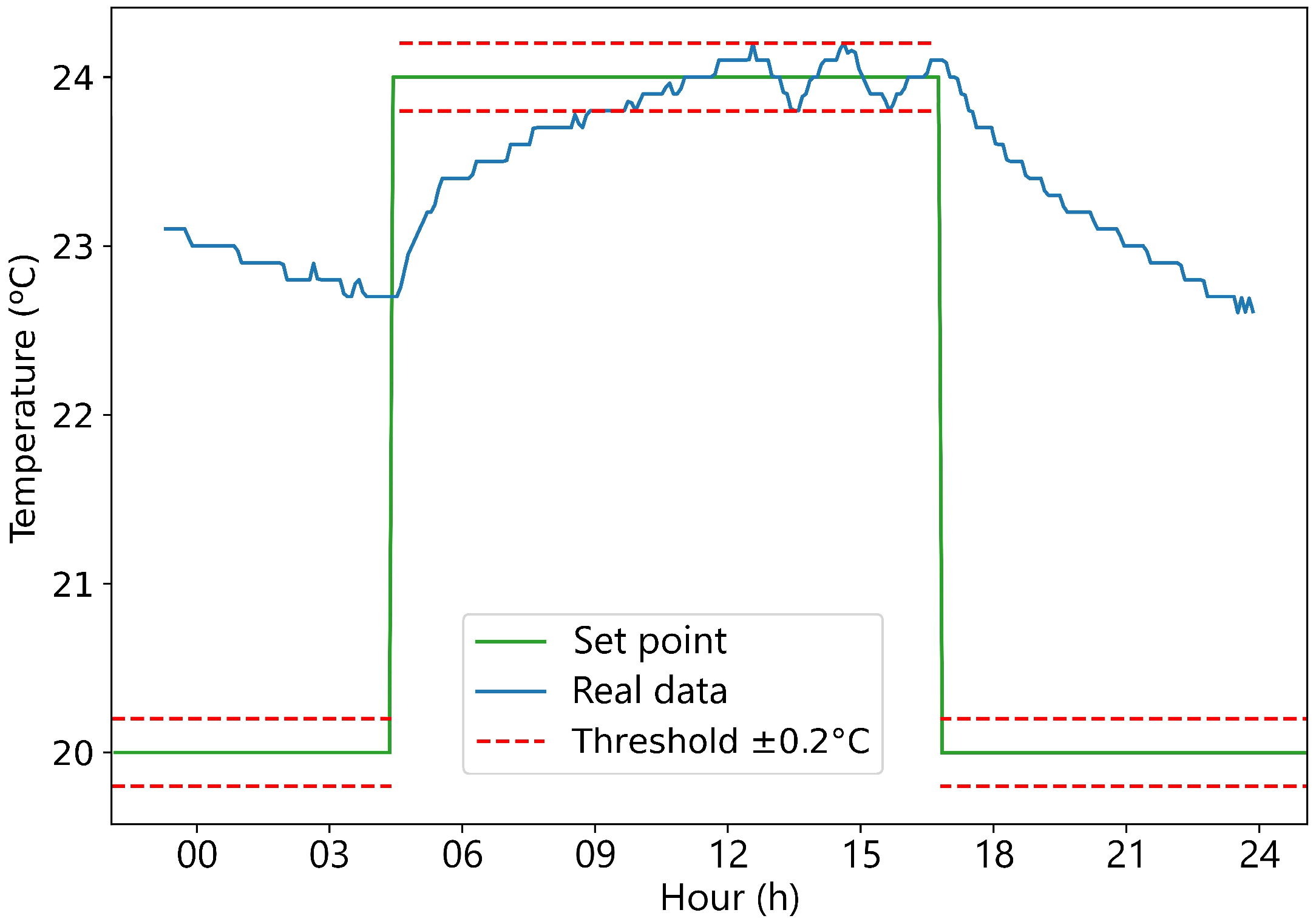
Section 4.3. This behavior can be seen in
Figure 8; when reaching the set point, it oscillates between the region defined by the thresholds. The values of the upper and lower bound are set manually to 0.2 °C for the laboratory.
Following Algorithm 1, the laboratory_tendency variable is build. This is based on the understanding that the temperature tendency during heating corresponds to the temperature of the inertia tank, as the hot air pumped by the fan coil is heated by the temperature of the inertia tank. Additionally, the energy consumption of the fan coil can also be predicted if a constant power consumption of 0.2 kW is assumed.
5.3.2. Inertia Tank Tendency Temperature
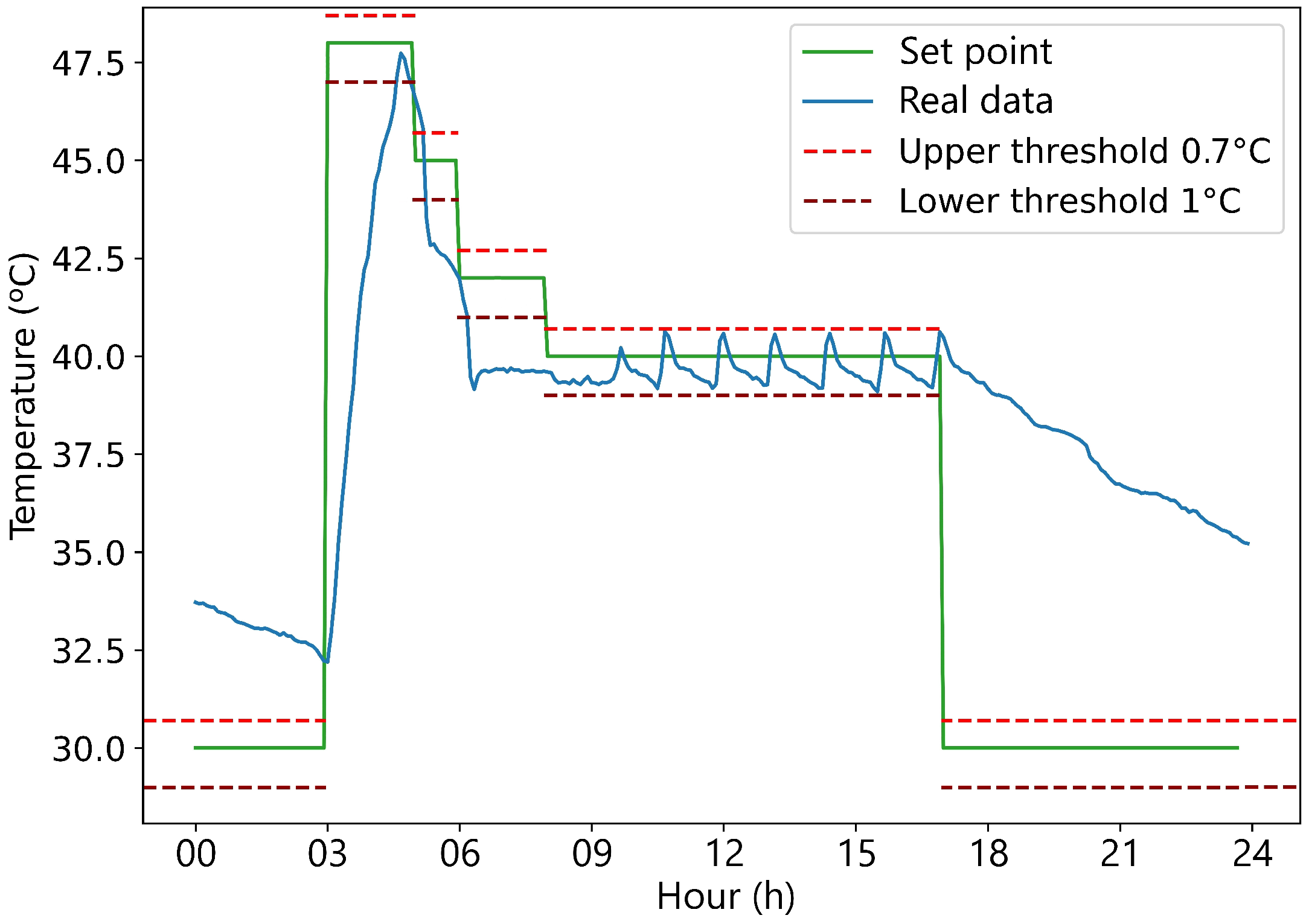
The inertia tank operates based on the same principles as the laboratory but with different values. It has a set point, meaning that if the tank’s temperature falls below this value, the heat pump is activated. The tank also has upper and lower thresholds. The tank heats to the set point plus the upper threshold, and once this value is reached, the heat pump turns off until the temperature drops below the set point minus the lower threshold. This behavior can be observed in
Figure 9 from 09:00 to 17:00. In this system, the upper threshold is set to 0.7 °C and the lower threshold is set to 1 °C.
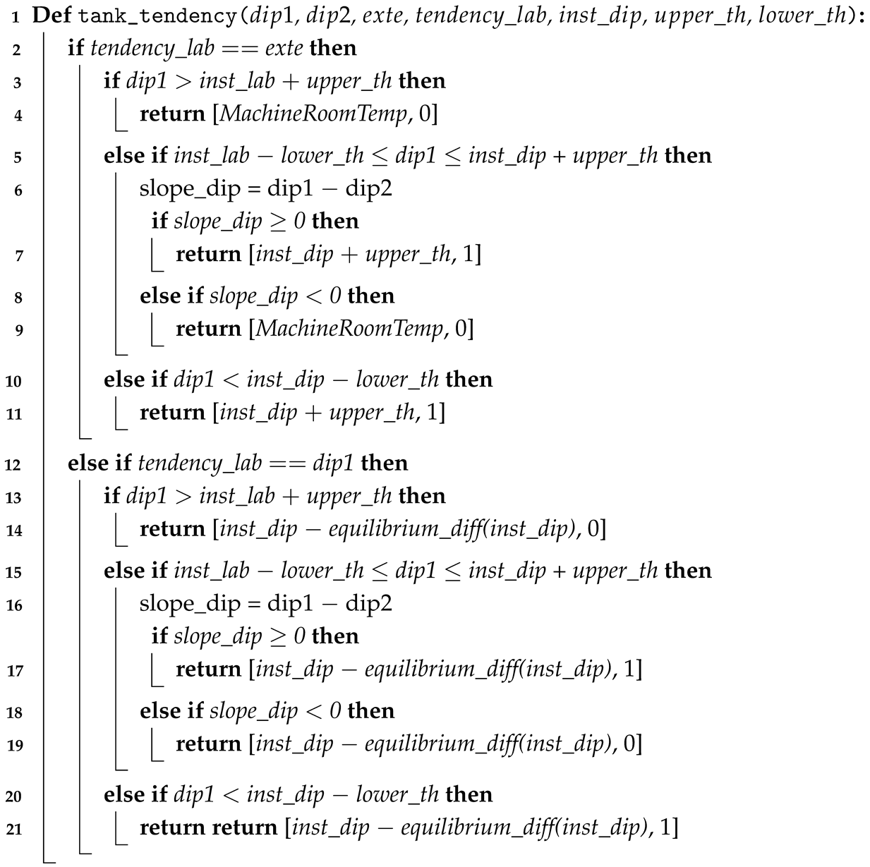
The laboratory only has two modes, either becoming hotter by the use of the fan coil or colder by the difference with the exterior temperature. For the inertia tank, the tendency function has to differentiate if the fan coil is ON or OFF. Four distinct modes are distinguished based on the status of the fan coil (ON/OFF) and the status of the heat pump (ON/OFF). If the fan coil is OFF, the behavior of the inertia tank is straightforward, resembling that of the laboratory. If the temperature is below the set point minus the lower threshold, it tends to be heated to the set point plus the upper threshold, if the temperature is above the set point, it tends to be cooled tending toward the temperature of the machine room, which is the environment with which the inertia tank is in contact. If the fan coil is ON, it is observed that the temperature of the inertia tank reaches a certain equilibrium temperature. This is due to a balance between the capacity of the fan coil to extract heat and the capacity of the heat pump to introduce heat.
Figure 10a,b show an example where the laboratory’s temperature is below the set point for long enough to observe how the inertia tank reaches a equilibrium temperature when the set point is at 40 °C from 08:00 to 17:00. Finding this equilibrium temperature is essential to define the tendency function of the tank.
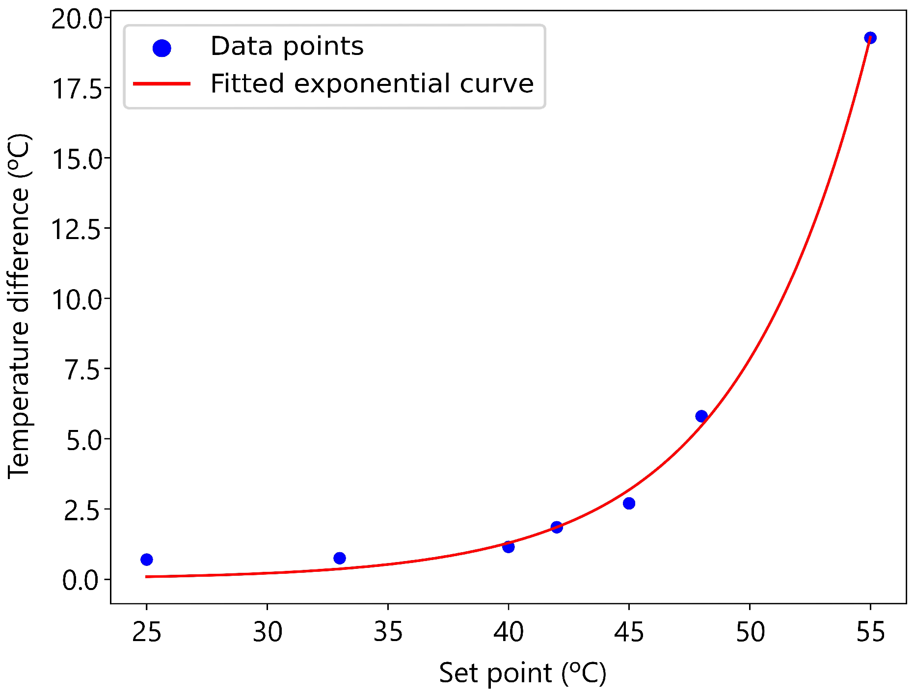
To identify the equilibrium temperature of the inertia tank, an alternative variable was chosen that expresses the same idea: the difference between the set point and the actual temperature. This approach offers greater utility by providing insights into temperature differences at low and high set points without directly involving the tank temperatures. The procedure was as follows: from the dataset, cases were initially selected where both the fan coil and the heat pump were activated; next, the temperatures of the inertia tank were classified according to their set points; following that, the difference between the set point and the tank temperature was computed, and only the positive values were stored. Because only temperatures below the set point are of interest, only positive differences were stored. The data obtained are shown in
Table 3.
The set points of 39.7 °C and 47.0 °C are identified as outliers that can be dismissed due to their low number of samples, which are considered non-representative. The remaining points in
Figure 11 follow an exponential function with the general expression
with
. Using the
curve_fit function from the
scipy.optimize package [
27], an exponential curve was successfully fitted to the data. The parameters
A,
b, and
c that best describe the fit were obtained and are presented in
Table 4. The resulting exponential curve is illustrated in
Figure 11.
With this curve, it is now possible to calculate the expected temperature difference that a set point should have with its corresponding equilibrium temperature when both the fan coil and heat pump are operational.
At this point, all necessary components are available to construct the tendency function of the inertia tank, which follows the structure presented in Algorithm 2.
| Algorithm 2: Temperature tendency of the inertia tank |
Input: dip1: Temperature of the tank at time t−1 dip2: Temperature of the tank at time t−2 exte: Exterior temperature at time t tendency_lab: Temperature tendency of the laboratory at time t inst_dip: Set point for the tank at time t upper_th: Upper threshold lower_th: Lower threshold Output: Vector: [Tendency temperature, 1 if heat pump is ON 0 if heat pump is OFF] |
![Applsci 15 04291 i002]() |
5.4. Laboratory Approximations
For the laboratory, the following features will be utilized: its own temperature, the set point temperature, the exterior temperature, the value of which can be known in the future using an API that communicates with the multiple weather applications that already exist, and the number of people inside the room. This last feature is the most difficult to know in the future since it involves human behavior, which tends to be hard to predict. Since the system is like an office and investigators follow a certain schedule, the number of people inside the room follows a certain pattern. Following
Section 4.1 of the methodology, the number of people inside the room is approximated simply by fitting a Gaussian
1 using the
cuerve_fit function.
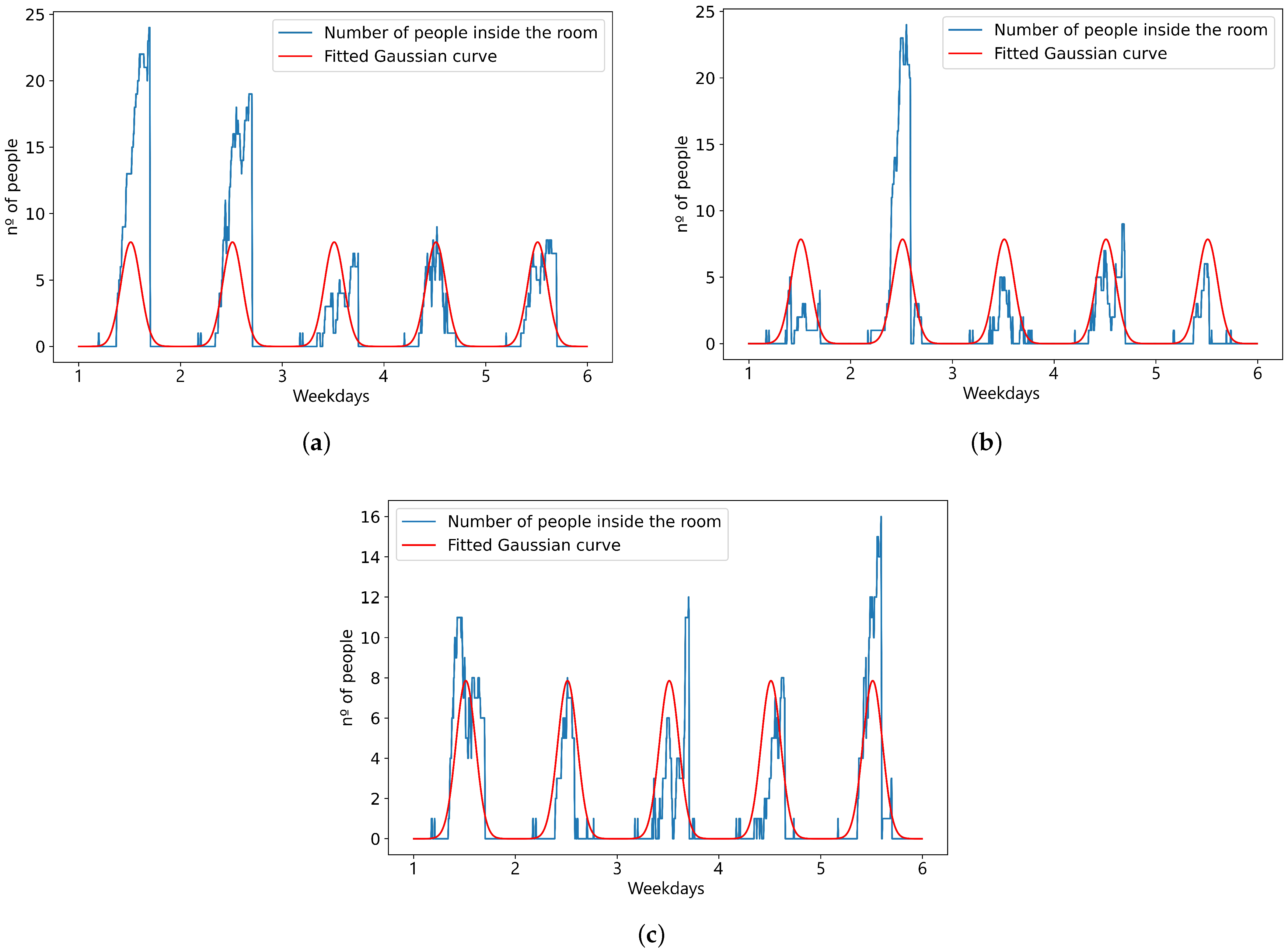
The door sensor is used to find the number of people inside the room. This sensor has a good performance when people enter or leave the room individually with spacing but when more than one person is involved, it has many counting errors. As an example, it is seen on certain days of
Figure 12a–c how the sensor can count up to 20 people or higher even if by experience it is known that usually there are not more than 7 people inside the room at any one time. Taking into account this consideration, the points with number of people above 7 are marked as outliers and are not used by the
curve_fit function.
The mean of each computed Gaussian value was taken to obtain a single function that approximates the number of people for each day for the test phase, and a Gaussian adjusted to each day was computed for the training phase. The parameters of the Gaussian found for the test phase are gathered in
Table 5 and visualized in red in
Figure 12a–c.
Table 6 summarizes all the features that will be integrated in the laboratory’s model. At first glance, it looks like it is missing a crucial value, which is the set point, but it is important to note that this information is actually integrated into the tendency variable.
The only approximation made is that the number of people inside the room follows a Gaussian distribution. For the training phase, the Gaussian distribution is computed daily to smooth the data. For the test phase, the Gaussian distribution used is the one provided in
Table 5.
5.5. Inertia Tank Approximations
For the inertia tank, the following features will be used: the temperature at past time instants and the tank’s tendency temperature, which encompasses multiple variables such as the set point, the exterior temperature, and the tendency temperature of the laboratory.
Table 7 brings together all the features that will be integrated for the inertia tank. Similarly to with the laboratory, the set point is hidden in the tendency variable.
The following approximations were applied in the development of the model: First, the temperature of the machine room was assumed to remain constant at 23 °C. Second, the equilibrium temperature, when both the heat pump and the fan coil are in operation, was calculated by approximating the difference between the set point temperature and the equilibrium temperature using an exponential function.
5.6. Model Selection
As seen in
Section 2.1, many models can be applied to forecast HVAC system temperatures, each with its pros and cons. In this study, data-driven models were chosen due to the quantity and quality of the data collected. To model the thermal systems, SVR was chosen for its robust performance in handling high-dimensional and non-linear data, which are characteristic of thermal systems. SVR employs a kernel to effectively map input features into higher-dimensional spaces where linear separation is feasible, thus capturing the complex, non-linear relationships of thermal dynamics. Additionally, SVR’s ability to minimize the generalization error ensures that the model remains accurate and reliable even with noisy data, which is common in real-world thermal measurements. Its intrinsic regularization mechanism prevents overfitting, making it suitable for predicting thermal responses under varying conditions.
The methodology is not restricted to SVR or a specific type of model. Instead, it is flexible and can accommodate any data-driven model that suits the characteristics of the data and the system being studied. This adaptability allows researchers to select models that align best with their data’s structure and the system’s requirements, fostering the exploration of diverse techniques for improved predictive performance.
6. Experiments and Results
The models generate predictions based on previously predicted data. As the forecast extends further into the future, errors accumulate, leading to a decline in performance. For this reason, predictions are limited to a 24 h timeframe. The performance of each forecasting model was evaluated using the metrics described in the previous section.
The first part is dedicated to the selection of the best hyperparameters for the forecasting of the laboratory, the second part is dedicated to the inertia tank, and the last shows the performance of both models working with each other. For both systems, the hyperparameters examined to find the best combination are the same:
Kernel = [, ]
C = [0.1, 0.5, 1, 5, 10, 25, 50, 100]
= [0.01, 0.05, 0.1, 0.5, 1, 5, 10]
= [, ]
6.1. Laboratory Modeling
Table 8 shows the five best models sorted by their averaged values of R
2. To allow comparison, standalone data-driven models underwent training using an identical grid search for hyperparameters. The top-performing model achieved an
of 0.33, revealing a weak relationship between the predicted and observed values.
The model with hyperparameters kernel = , C = 1, = 0.05, and = demonstrated superior performance by achieving the highest and metrics.
However, the analysis indicates that the
values are notably low, suggesting that the model may not be effectively capturing the relationship between predictors and response variables.
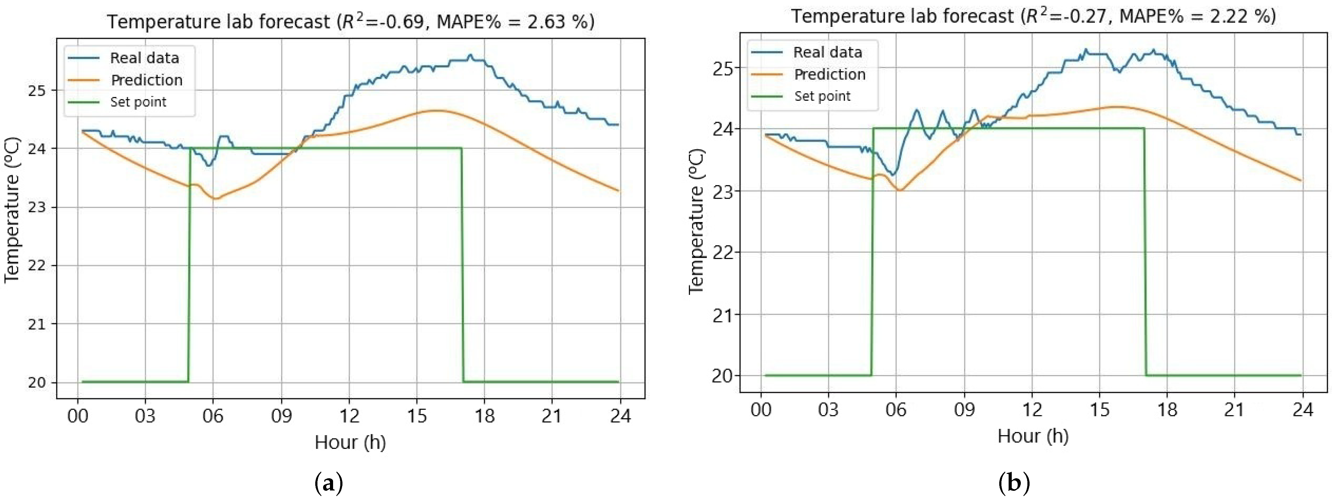
Table 9 provides a detailed examination of the daily performance, revealing that the R
2 values experienced significant declines on two specific days, thereby impacting the overall
. Despite this, the
values remain exceptionally low, which attests to the model’s high accuracy and reliability.
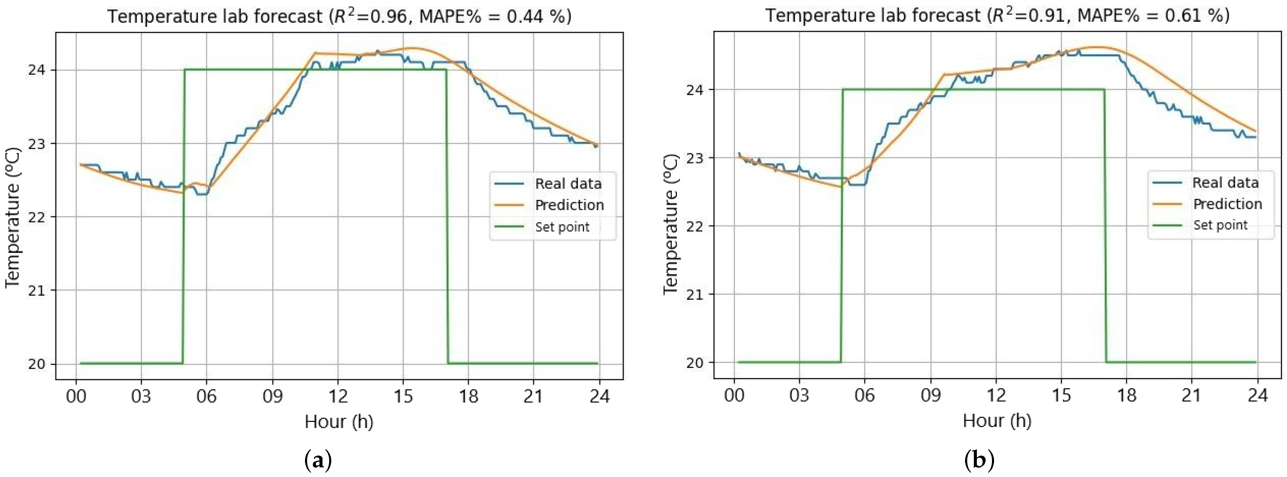
Figure 13a,b illustrate these days of suboptimal performance.
Aligning these underperforming days with unusually hot weather explains the reduced model performance. Despite low R
2 values, the prediction profile reveals a reasonably accurate curve, with larger deviations typically around 1 °C. In contrast, the best-performing days with the highest R
2 values and lowest MAPE scores are shown in
Figure 14a,b.
Obtaining a negative R2 score but a very low MAPE is unusual but can occur due to significant variance differences between training and test datasets. While the test data’s high variability challenges the model, resulting in worse performance than mean-based predictions (negative R2), the low MAPE indicates reasonably accurate predictions in regions where test and training data variability align. The model captures overall trends but struggles with local variations or outliers.
6.2. Inertia Tank Modeling
Table 10 lists the five top models sorted by their average R
2 values (
). For comparison purposes, standalone data-driven models were trained using the same grid search of hyperparameters. The model with the best performance achieved an
of 0.16, indicating a weak correlation between the predicted and observed values.
For both and , the best hyperparameters are kernel = , C = 50, = 0.05, and = .
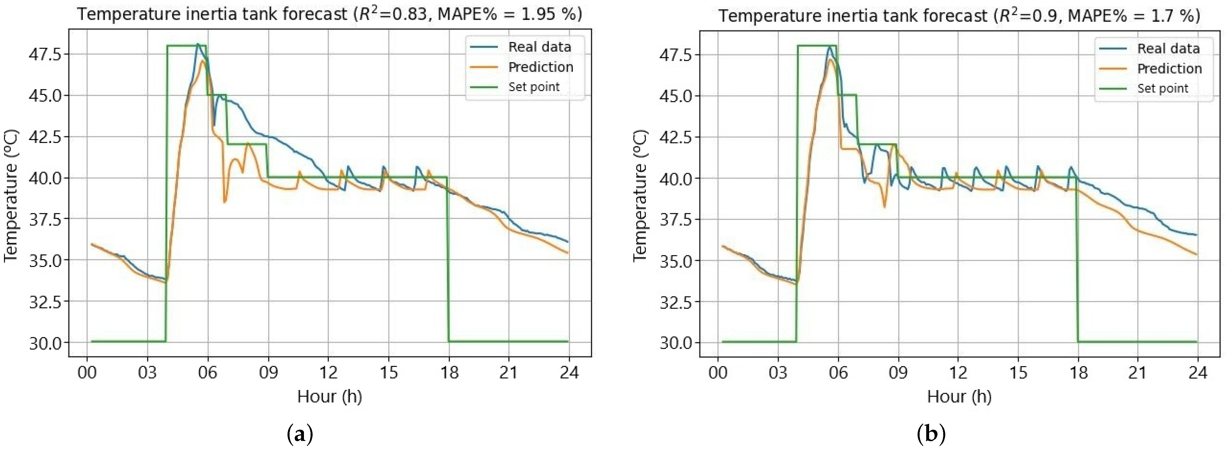
The observed deviations in the laboratory temperature cannot be extrapolated to the inertia tank temperature. This is because the inertia tank is more insulated than the laboratory and less susceptible to external temperature fluctuations. Additionally, the variables influencing the behavior of the inertia tank are not subject to randomness or hard-to-predict factors, such as laboratory occupancy. Consequently, the models achieve higher R
2 values and lower MAPE scores for each day tested, as shown in
Table 11.
Figure 15a,b illustrate the two worst-performing days.
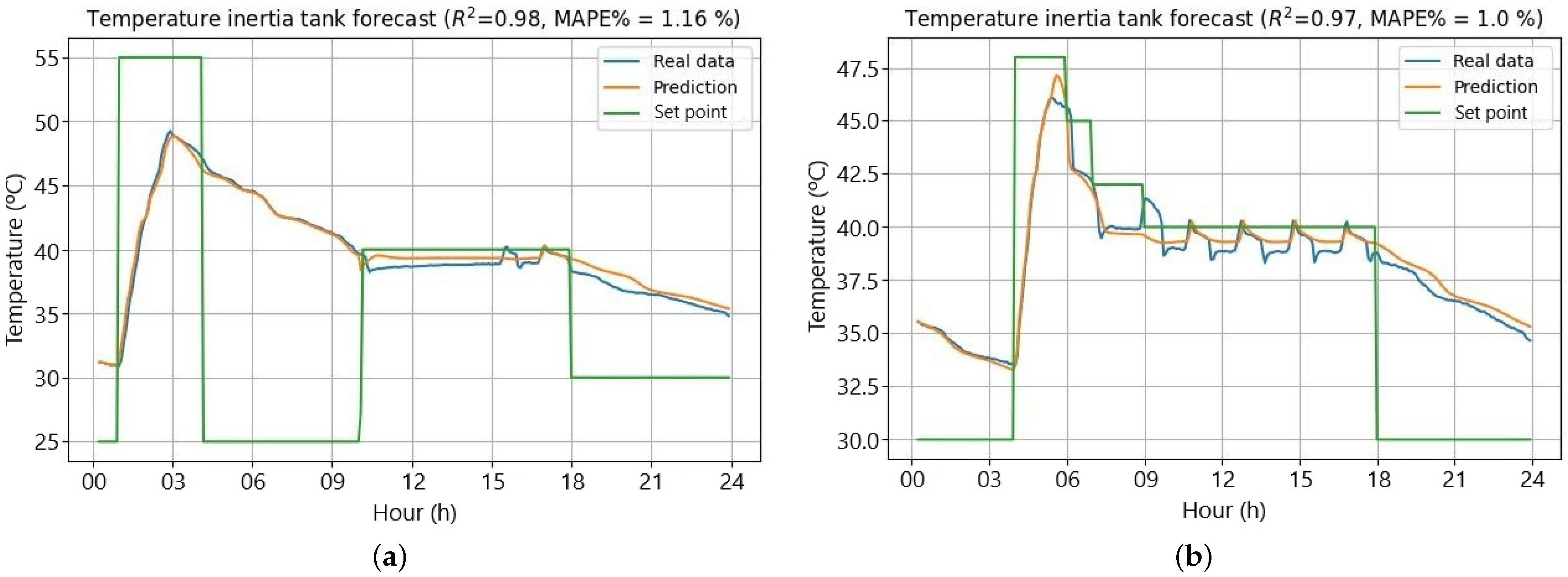
Even though the last figures were the worst predicted, the values taken by their score metrics indicate a good fit, with high accuracy also shown by the prediction profile of the temperature.
Figure 16a,b show the best predicted values of the test set.
6.3. Combination of the Two Models
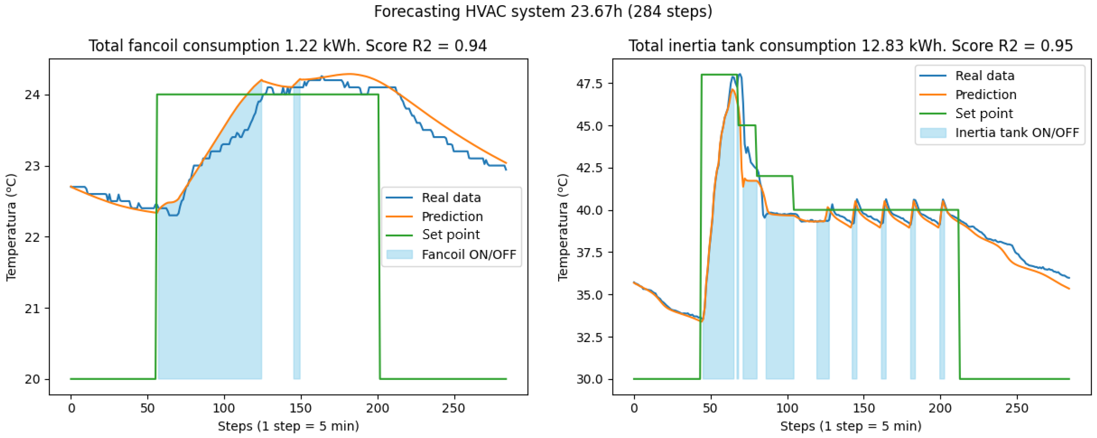
Forecasting temperatures for both the laboratory and the inertia tank is possible by integrating the outputs of two models, using each prediction for the next time instant’s temperature. This method relies on the set points for both systems and the exterior temperature, the latter being the only constraint. On the test set, the combined models achieve an of 0.91 for the inertia tank, consistent with previous performance. The fan coil, however, shows an of 0.37, worse than the standalone model. Examining individual test days reveals the highest errors occur on days with the greatest deviations. Excluding these two days improves the to 0.79, confirming the model’s robust performance on other days.
Although this study does not primarily focus on energy consumption forecasting, such an analysis can be conducted by assuming constant power operation at 0.2 kW for the fan coil and 2 kW for the inertia tank. The operational status of the machines, as indicated by tendency variables, allows the determination of total energy consumption.
Figure 17 and
Figure 18 illustrate the optimal forecast days within the combined model’s test set, with blue shaded areas indicating periods of system operation.
Zhao et al. [
47] focused on forecasting room temperature in HVAC systems by leveraging historical data to identify distinct operational scenarios using k-means clustering. These scenarios, representing different modes of operation (e.g., cooling or heating), are used to train separate temperature prediction models via symbolic regression. The methodology was tested in a lecture building in Suita, Osaka, Japan, using data collected at 5 min intervals over a year from multiple indoor and outdoor sensors. The best results achieved were an R
2 of 0.97 for the cooling phase and 0.73 for the heating phase.
The study described in [
47] closely resembles the system under investigation, with the primary difference being the absence of geothermal energy as a power source. Compared to this approach, our proposed methodology achieves superior accuracy in temperature forecasting for complex HVAC systems. While the clustering approach facilitates modeling through operational segmentation, it relies heavily on extensive datasets (over 232,576 data points) and may struggle to generalize in scenarios with limited data availability or unique configurations. In contrast, the proposed approach explicitly integrates domain knowledge, allowing the model to achieve R
2 values of 0.94 for the laboratory and 0.93 for the inertia tank even when using the combination of the two models, independently of the operational mode and with much less training data. The integration of physical principles enhances model reliability, ensuring the forecasts remain grounded in the underlying thermal dynamics. Moreover, the adaptability of our methodology makes it more reliable, demonstrating how it can handle complex HVAC systems and improve accuracy in real world scenarios
7. Conclusions
This work introduced a general methodology for a feature selection and extraction approach based in physical equations and expert knowledge of HVAC system logic to create new variables highly influential to model performance.
The methodology used for constructing tendency variables allows precise computation of the energy consumption for each machine and accurate temperature predictions. The results demonstrate the effectiveness of the proposed method, showing how leveraging physical principles can enhance both the accuracy and flexibility of the models.
The performance of the models for both the laboratory and the inertia tank heavily depend on the availability of a high-quality and sufficiently large dataset for training. Without a proper dataframe, both in terms of data quality and quantity, the accuracy of predictions may be compromised. In systems influenced by factors that are poorly registered or are not even available, such as occupancy levels or solar irradiation, among others, the model may struggle to make precise predictions if these variables are not adequately represented in the training data. An example of this can be seen in the modeling of the inertia tank, where we achieved higher accuracy compared to the laboratory’s model. The laboratory’s model is influenced by variables that are both significant and challenging to predict, such as occupancy levels or solar irradiation, among others, whereas the inertia tank, being a more isolated system, is not affected by such uncertainties. Nevertheless, the proposed models exhibit promising results and there are opportunities for improvement. Enhancing the forecasting of the occupancy levels with other non-linear equations or machine learning models, could lead to more accurate temperature predictions of the laboratory. Additionally, developing a model to predict the temperature of the machine room, where the inertia tank is located, which is currently assumed to be constant but actually fluctuates, would further enhance the model’s accuracy and applicability.
The results obtained for the standalone modeling of both systems showcase the limitations of the models and, more importantly, highlight the added value of the proposed novel preprocessing methodology. This approach emerges as a promising tool for improving the quality and precision of temperature and energy consumption of HVAC systems. Furthermore, the proposed methodology, based on physical equations, can be generalized to other fields with sufficient expert knowledge about the system under study, making it a valuable approach for future research.
Future work will expand by applying the proposed methodology to a wider array of data-driven models, aiming to develop more accurate dynamic temperature profiles. Additionally, these models will be integrated with optimization algorithms to minimize energy consumption, achieve cost savings, and maintain comfortable indoor temperatures.


