Ultrasound Reconstruction Tomography Using Neural Networks Trained with Simulated Data: A Case of Theoretical Gradient Damage in Concrete

Abstract

Gradient damage processes in cementitious materials are generally produced by chemical and/or physical processes that travel from outside to inside. Depending on the type of damage, it can cause different effects such as decreased porosity, cracking, or steel corrosion in the case of carbonation, or increased porosity, micro-cracks, expansion, and spalling (also present in thermal damage) in the case of external attack by sulphates or acid attack. Therefore, estimating the boundaries of this damage is an essential task for concrete quality assessment. The first objective of this work was to use neural networks (NNs) for ultrasound tomographic reconstruction of concrete samples in order to estimate the advance front in gradient damage. Unlike the usual X-ray tomography, ultrasound tomography is affected by diffraction, among other factors. NNs can learn to compensate for these effects; however, they require a large amount of training data to achieve accurate results. In the case of cement-based materials, obtaining and measuring a real training database could be complicated, expensive, and time-consuming. For this purpose, a training process using simulated measurements was carried out. The second objective of this work was to demonstrate the feasibility of training neural networks through simulations, which reduces costs. Finally, the trained neural network for tomographic reconstruction was evaluated using real cylindrical concrete specimens. Each specimen consisted of an outer cylinder, representing externally exposed cement, and an inner cylinder, simulating the unaffected core. The Structural Similarity Index (SSIM) was used as a metric to assess the reconstruction accuracy, achieving values of 0.95 for simulated signals and up to 0.82 for real signals.

1. Introduction

Cement is one of the most widely used materials in construction due to its versatility, strength, and durability. Furthermore, as a primary component of concrete and mortar, it plays a critical role in the development of building structures. Its workability and ability to harden and gain strength over time makes it indispensable for creating long-lasting and resilient structures, ensuring its continued importance in the construction industry around the world.

However, cement-based materials are exposed to a variety of physical and chemical disturbances that could affect their properties during their service life. These disturbances often induce some kind of deterioration, which manifests itself as external or internal pathologies, ultimately compromising the material’s mechanical properties.

Among the numerous damage mechanisms affecting cementitious materials, gradient damage processes are particularly significant [1,2] and arise from variations in temperature, humidity, or chemical reactions within the material. Notably, these deterioration processes typically propagate from the exterior towards the interior of the material and can be broadly categorized into chemical types (e.g., external sulfate, acid attacks, and carbonation) and physical types (e.g., high-temperature exposure).

In the context of physical damage, high-temperature exposure alters the hydration products of cement [3], producing microcracks within the matrix and at the aggregate–matrix interface. These alterations reduce their mechanical properties such as compressive strength, hardness, and elastic modulus.

In the context of chemical attacks, carbonation is a natural chemical reaction which occurs when carbon dioxide (CO₂) in the air reacts with hydrated cement compounds, forming calcium carbonate (CaCO₃). The formation of calcium carbonate produces a densification (reduction in porosity) of the cementing matrix and creates a pH gradient [4]. The pH reduction undermines the passive layer protecting the embedded steel reinforcement, exposing it to corrosion in the presence of moisture and oxygen. Taking this into consideration, the corrosion products, predominantly rust, occupy a larger volume than the original steel, causing internal stress that results in cracking, spalling, and a significant decrease in structural integrity.

This interplay of physical and chemical disturbances underlines the necessity of understanding and estimating the gradient damage in order to enhance the durability and performance of cement-based materials. Previous studies on non-destructive testing have extensively utilized ultrasonic techniques to detect and evaluate damage in concrete arising from this type of pathology. Moreover, these studies predominantly employed ultrasonic velocity as a diagnostic parameter to determine the differences between damaged and undamaged samples. For example, in [5], the carbonate front was successfully estimated using Quantitative Ultrasound Imaging (QUS) with high-frequency ultrasound signals (2.5 MHz). This method leverages an array of transducers and the analysis of microstructural information through backscattering and attenuation coefficients.

Another approach to identifying damaged regions involves ultrasonic tomography, which irradiates the specimen from multiple positions [6]. The collected signals form projections, which enable the generation of visual cross-sectional images of the material using reconstruction algorithms, all without causing any damage. Since its beginnings, tomography has played a crucial role in quality control and is used in multiple disciplines such as medicine, archaeology, biology, geophysics, oceanography, and science, among other disciplines. Tomographic reconstruction algorithms can be categorized into three primary groups: transformed, algebraic, and machine-learning-based techniques.

Transformed algorithms reconstruct images by applying the Fourier Slice Theorem [7] to projections. Techniques such as the Direct Fourier Transform [8] and the Filtered Backprojection Method [9] are included in this category. These methods are effective when the irradiation rays do not experience diffraction and data are abundant, as they require a high number of directions and rays to produce high-resolution images.

Algebraic methods approach reconstruction as a linear system problem, where the object’s cross-section is represented by an array of unknowns derived from measured projections. In this sense, these methods are advantageous when data are limited, making them suitable for scenarios with reduced projections, low resolution, or complex geometries. Regularization techniques are often incorporated in order to improve image quality. Among the most widely studied and utilized methods are the Algebraic Reconstruction Technique (ART) [10] and Simultaneous Iterative Reconstruction Technique (SIRT), [11] along with their numerous variants detailed in the literature such as the Controlled Algebraic Reconstruction Technique (CART) [12] and Simultaneous Algebraic Reconstruction Technique (SART) [13]. However, they have the main limitation of a high computational cost when large reconstructions are required [14,15]. Additionally, parameters such as the relaxation rate or the number of iterations can affect the stability and accuracy of the results from these methods, and it is not always easy to determine the optimal values [16].

Advancements in machine learning have opened new avenues for tomographic reconstruction, with artificial neural networks (ANNs) playing a prominent role. Generally, two principal approaches to neural network integration have been identified. In the first approach, post-processing enhancement, ANNs are employed to refine reconstructed images and mitigate artifacts produced by conventional reconstruction algorithms [17]. For instance, a Convolutional Neural Network (CNN) model was used in [18] to detect cracks and faults in tomographic reconstructions. Similarly, in [19], a CNN was trained to enhance reflection tomography images obtained via idealized back-projection. Moreover, U-Net architecture has been applied to the segmentation of reconstructed images [18,19]. The second approach, end-to-end reconstruction, involves the development of neural network models that process raw projection data to directly generate reconstructed images. For example, Ref. [20] employed a Multi-Layer Perceptron (MLP) to map Time-of-Flight (TOF) ultrasound measurements into defect images for reinforced polymer composites. Others, like [16], used the structure of MLP combined with an iterative reconstruction algorithm (named MLP-BPE), and tested damaged mortar specimens. Additionally, in [21], a Radial Basis Function Neural Network (RBFNN) was proposed to map different parameters (ultrasonic velocity, signal attenuation, and centroid frequency). This model demonstrated precise reconstruction capabilities in damaged specimens, including aluminum alloy and concrete specimens, which were validated using both simulated and experimental data.

Despite the promising accuracy and efficiency offered by neural networks, both approaches demand substantial volumes of data for model training. Furthermore, this requirement becomes increasingly pronounced as the neural network model complexity grows. Obtaining real-world samples of damaged cement is a costly and resource-intensive task.

In this study, we proposed the application of a neural network for tomographic reconstruction of damaged cylindrical mortar samples, with training conducted on simulated datasets. This approach addresses a significant limitation of conventional reconstruction algorithms, which normally assume a straight-line wave propagation, neglecting the diffraction and refraction effects from ultrasonic waves. Thus, our model employs a simplified feed-forward neural network architecture with a single hidden layer (although alternative configurations were explored) to adapt the reconstruction process to the complexities of wave propagation in damaged materials. Moreover, validation of the model was carried out using synthetic “embedded mortar” samples generated in the laboratory, which were designed to emulate realistic cases of concrete with gradient damage. In this regard, these synthetic samples were controlled specimens with varying densities, closely mimicking the properties of gradient-damaged concrete.

This article was organized as follows: First, we provide a concise theoretical introduction to the critical parameters for tomographic reconstruction, including projections, directions, and rays. Secondly, the design and characteristics of our neural network model are described. Following this, we detail the experimental methodology, encompassing the training, validation, and evaluation processes conducted with both simulated and real-world data. The training phase focused on simulated data, as it offers a controlled and scalable environment for model development. Finally, we present our results, accompanied by a discussion of the reconstruction quality and its implications, and concluding with insights and potential areas for improvement.

2. Theoretical Background

Tomography is a non-destructive process used to obtain cross-sectional or three-dimensional images of the interior of a given inspected material. This technique is based on radiating the body from different angles, followed by a mathematical procedure called tomographic reconstruction, which is responsible for carrying out the internal reconstruction using the received signals and visualizing the representation of a cross-section or slice of the scanned body.

This work used ultrasonic signals to obtain tomographic images. Ultrasonic signals are not ionizing waves and do not pose a health risk to people; this makes it, despite its disadvantages, one of the most widely used methods of excitation for inspection in general non-destructive testing. Thus, the use of ultrasonic imaging to assess the quality and degradation of concrete structures by identifying heterogeneities, defects, or cracks is a very attractive solution for the diagnosis of civil infrastructures [22,23]. However, a problem arises when using ultrasonic signals as the excitation method because traditional reconstruction algorithms are designed for excitation using X-ray sources, using the attenuation coefficient. These X-rays do not diffract, allowing them to travel in a straight line, which does not occur when the excitation source uses ultrasonic waves or microwaves; when the wave collides with a heterogeneity, it is scattered in practically all directions and only under certain conditions can we assume that the propagation line of the ultrasonic wave is practically straight. This demonstrates that, in certain cases, classical algorithms are not suitable for ultrasonic reconstruction and that neural networks could compensate for these shortcomings.

2.1. Projections, Rays, and Sinograms

The results of tomography mainly consist of projections. These are sets of measurements produced by integrating along straight lines through an object. This integral is defined as the integral of a certain parameter of the object along a line (Equation (2)) like velocity and attenuation. These straight lines are called rays and are determined using Equation (1):

$$x·\cos \left(\theta \right)+y·\sin \left(\theta \right)=t$$

(1)

The definition of the integral line could be written as

$$P_{\theta }\left(t\right)={\int }_{{\left(\theta ,t\right)}_{line}}f\left(x,y\right)dS$$

(2)

where $f\left(x,y\right)$ is a two-dimensional function that models the object under study. Expressing the previous integral as a double integral, we obtain Equation (3), where the function $\delta$ represents the Dirac delta function.

$$P_{\theta }\left(t\right)={\int }_{-\infty }^{\infty }{\int }_{-\infty }^{\infty }f\left(x,y\right)·\delta \left(x·\mathit{cos}\left(\theta \right)+y·\mathit{sin}\left(\theta \right)-t\right)dxdy$$

(3)

where function $P_{\theta }\left(t\right)$ is known as the Radon transformation [9] and describes the relationship between the object to be reconstructed and its projections. In this sense, a projection is formed by a combination of line integrals, as seen in Figure 1. The projection is a set of parallel rays for a constant θ. To obtain the rest of the projections, the source and detector are moved around the object.

Transmission tomography was used in this work. The selection of this type of tomography restricted the implemented measuring system, in which two transducers face each other, one acting as the transmitter and the other as the receiver. Although the classical projection definition defines parallel rays, it could be redefined as the path connecting the transmitter to the receiver. Likewise, there are different types of projections depending on the direction and distribution of these rays. Although it is simpler to implement the parallel ray structure (see Figure 1a), a fan ray structure was selected due to the circular shape of the specimens. The transmitter and receiver positions were angularly equidistant (Figure 1b). Each projection was achieved by placing the transmitter in one position and moving the receiver by a certain angular increment. This was repeated for all possible positions of the transmitter, around the object under study, but it produced a low density of rays in the central part and a very high density in the outer part. For an object (Figure 2a), if the projections are arranged according to the different directions in which the object is illuminated, the sinogram will be a two-dimensional representation (Figure 2b). Therefore, for a constant θ, if we went through all the possible positions, we would obtain a representation of the projection for that angle, as seen in Figure 2c, where we can observe the corresponding cuts in the directions of 120 and 40 degrees, respectively.

2.2. Neural Networks

Artificial neural networks (ANNs) are a set of computational systems inspired by the structure and functioning of biological neural networks. As ANNs are an analogy of the human brain, each of these simple processing units is called a neuron. Furthermore, each neuron receives a linear combination ($W·X$) of multiple input signals $\left(X\right)$, which serves as the input to the activation function ($f\left(\cdot \right)$), producing a single output signal ($f\left(W·X+b\right)$) that mimics the behavior of a biological neuron (Figure 3). An ANN is, therefore, a network composed of numerous simple processing units operating in parallel, whose functionality is determined by the network’s architecture, the strength of the connections (synaptic weights), and the processing rules applied by individual neurons in each node (Figure 4).

In essence, artificial neural networks are able to learn from empirical data, retain this learned knowledge, and apply it to perform specific tasks. They are characterized by a high degree of interconnection among simple processing elements and the capacity for adaptive interactions, enabling the network to adjust its synaptic weights. This adaptability allows ANNs to effectively handle uncertainty, noise, and probabilistic information, as well as to generalize insights from diverse input examples (Figure 4).

There are different types of neural networks. The simplest one is the Feedforward Neural Network (FNN) where the information flows unidirectionally from the input layer through hidden layers to the output layer. These networks are predominantly used for classification and regression tasks. Convolutional Neural Networks (CNNs) are optimized for processing grid-structure data such as images. They utilize convolutional layers to learn spatial hierarchies of features, making them ideal for image recognition and object detection. Recurrent Neural Networks (RNNs) can deal with sequential data by introducing feedback connections to process sequential data. They are widely used in tasks like time-series predictions and speech recognition. Autoencoders are specialized architectures comprising an encoder that compresses input data and a decoder that reconstructs them. They are primarily applied in data compression and noise reduction [24]. Generative Adversarial Networks (GANs) consist of a generator network and a discriminator network that are trained simultaneously. This kind of network is used for generating realistic images, data synthesis, etc.

Despite their structural and functional differences, all neural network architectures share a common characteristic: the necessity of a training process in order to learn from data. Training involves optimizing the network’s parameters (weights and biases) to minimize the error between predicted outputs and actual target values within a given dataset.

The implemented neural network structure in this work corresponds to a Multilayer Feedforward Network (Figure 4) characterized by the inclusion of one or more hidden layers. The function of these hidden layers is to serve as intermediaries between the network’s external inputs and outputs. Adding one or more hidden layers enables the network to extract higher-order statistical features due to both the extra synaptic connections and the large dimensions of the neural interactions. The capacity to capture higher-order statistics is particularly advantageous when working with high-dimensional input data.

The source nodes of the input layer of the network are fed by the activation patterns (input vectors), which constitute the signals applied to the second layer (called the first hidden layer). The output signals from the second layer are used as inputs to the third layer, and so on. Normally, the neurons in each layer only have the outputs of the previous stage as inputs. The set of output signals from the last layer constitutes the generated response of the network to the activation pattern supplied by the nodes of the input layer. Figure 4 shows an example of the structure of a neural network.

The learning process involves adjusting the synaptic weights between layers. This adjustment enables the neural network to optimize its performance by minimizing the error between the predicted and actual outputs. We used the stochastic gradient descendent [25,26] learning algorithm, with backpropagation of the error that consisted of a supervised learning algorithm, in which the error between the predicted and actual outputs is calculated. This error is propagated backward, updating the weights and reducing the error iteratively.

The objective of our neural network is to perform tomographic reconstruction from ultrasonic projections, and for this purpose, our inputs were the projections (sinograms), while the outputs were the reconstructed images associated with the projections (see Figure 4). However, one of the main challenges of neural networks is obtaining enough training examples. Therefore, training with real samples could entail a very high cost in terms of both time and money. In this article, as noted, we propose training the neural network with simulated cases in order to reconstruct real cases. For this purpose, some experiments were performed to test the reconstruction method, as discussed in the following section. During the training process, the inputs were our projections or sinograms, while the outputs were the images used to generate the simulated sinograms (with the assignment of different materials based on colors).

3. Materials and Methods

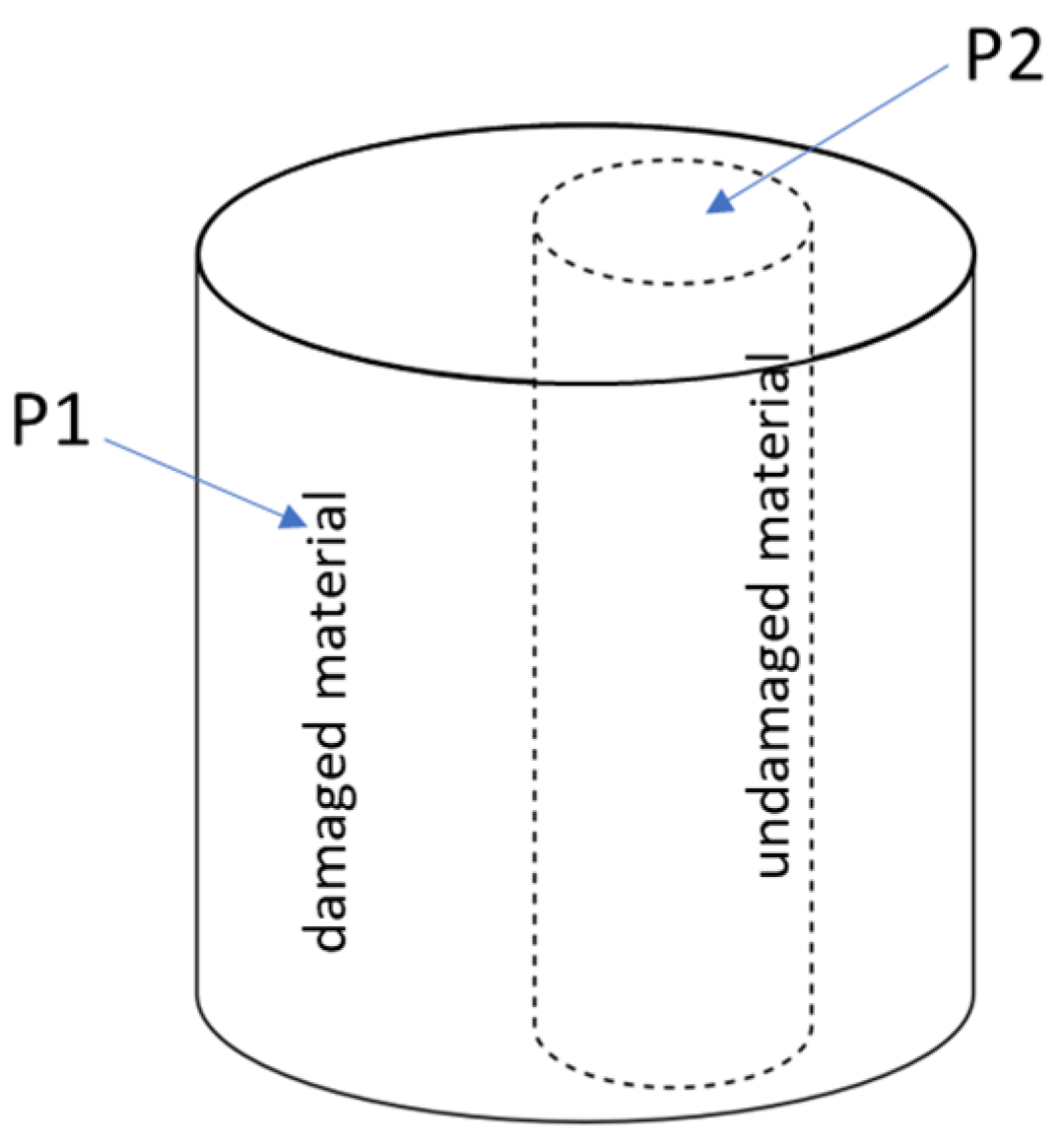
Damage caused by gradients in cementitious materials is typically manifested as a progression of damage from the exterior surface inward, gradually penetrating the material. Therefore, objects with a cylindrical shape were selected, with a P1 material representing the damaged outer material and P2 material representing the undamaged inner material (see Figure 5).

3.1. Fabrication Process

The experiments consisted of the fabrication of four mortar specimens (10 cm diameter and 20 cm height). The cement used was CEM I 52.5 R [27] (Cementval, Puerto de Sagunto-Spain). The mortars were composed of 1 part cement and 3 parts standardized sand [28] (Normensand, Beckum-Germany). The mortar mixing procedure followed the UNE-EN 196-1 standard [28], except for the quantity of water. 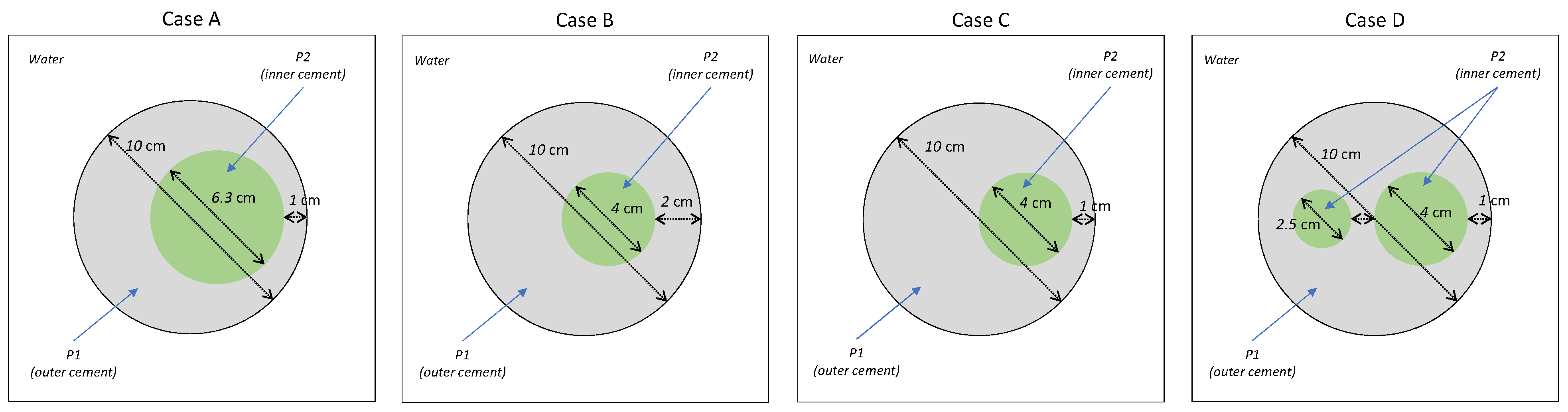Two types of mortars were prepared with different water/cement ratios: 0.6 for the internal material (material P2) and 0.35 (material P1) for the external material, as shown in Figure 5. The difference in the water/cement ratios for P1 and P2 resulted in different densities (simulating a carbonated zone with a higher density and a non-carbonated zone with a lower density). Additionally, prismatic mortar samples were prepared with the same ratios: these specimens were employed to measuring the ultrasonic pulse velocity (UPV), compressive and flexural strengths, and density, as well as the elastic constants of the materials. Their dimensions were 4 cm × 4 cm × 16 cm.

To make the different embedded cylinders, we used a cylinder as the mold for the 10 cm specimen and PVC pipes as the mold for the internal cylinders. According to these diameters, we numbered the specimens as follows (see Figure 6):

• Specimens with only one inner cylinder

  ○

  A (Ø 6.3 cm).

  ○

  B and C (Ø 4 cm).

• Specimen with two inner cylinders

  ○

  D (Ø 2.5 cm + Ø 4 cm).

The mortars were prepared by mixing Portland cement (CEM I 52.5 R type), water, and aggregate. The cement/aggregate ratio was 1/3 by mass. Furthermore, the mortar for inner cylinders was doped with 1% inorganic pigment (G&C Colors SA, Ceutí-Murcia) in order to facilitate the identification of the position of the cylinder after curing.

The properties of the prismatic mortar specimens, which we will call P1 and P2 (see

Table 1. Characteristics of P1 and P2 mortars: ultrasonic pulse velocity (UPV), compressive and flexural strengths, and density (measured on prismatic 4 × 4 × 16 cm³ specimens).

	$\mathbf{UPV} (\mathbf{m}/\mathbf{s})$		Mechanical Strengths		Density $[\mathbf{k}\mathbf{g}/{\mathbf{m}}^3]$
Material	Longitudinal	Transversal	Flexural [MPa]	Compressive [MPa]
P2	4121.58	2522.86	9.42	59.82	2190.46
P1	4807.69	2882.88	13.32	90.45	2329.53

), were measured.

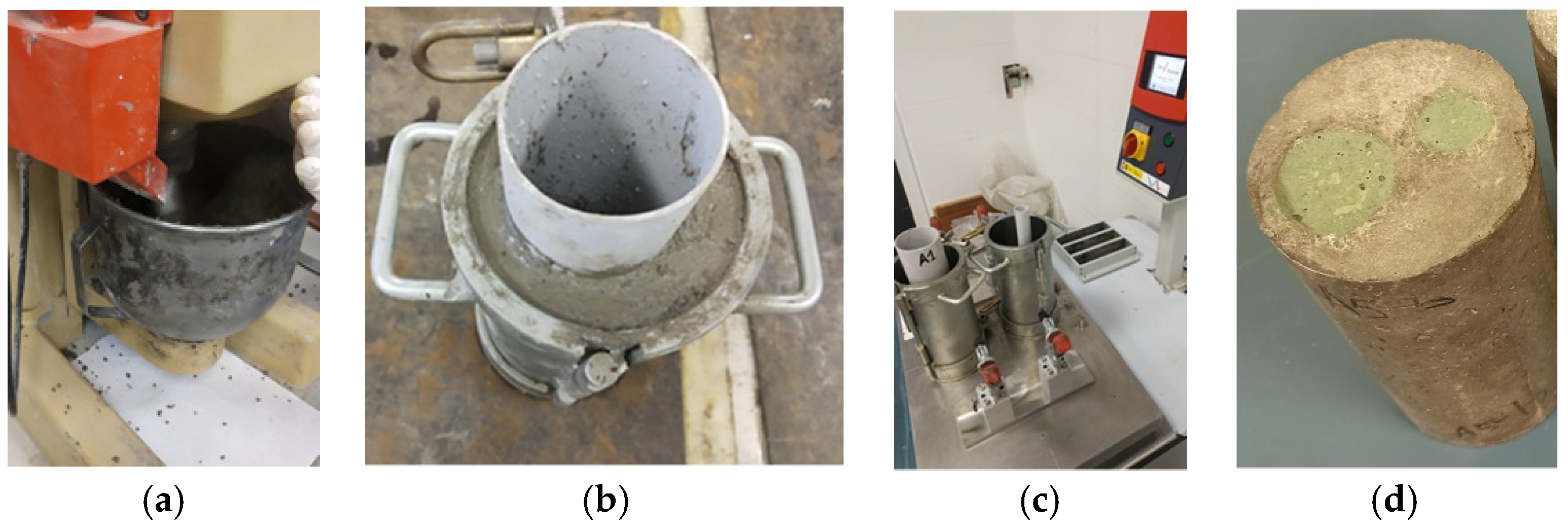
After weighing the proportions of sand, water, and cement, the specimens were prepared and the materials were mixed (Figure 7a) according to the UNE-EN 196-1 standard.

To embed them inside the larger mold (Figure 7b), we used a PVC cylinder for each internal cylinder. The outer material was first kneaded and then filled with the inner material. During the entire pouring process, the material was compacted and settled with a vibrator (Figure 7c). To distinguish between materials, we used green colorant, as shown in Figure 7d.

After that, all the specimens were stored in a high-humidity chamber, where they were completely cured for 28 days.

3.2. Real Measurements

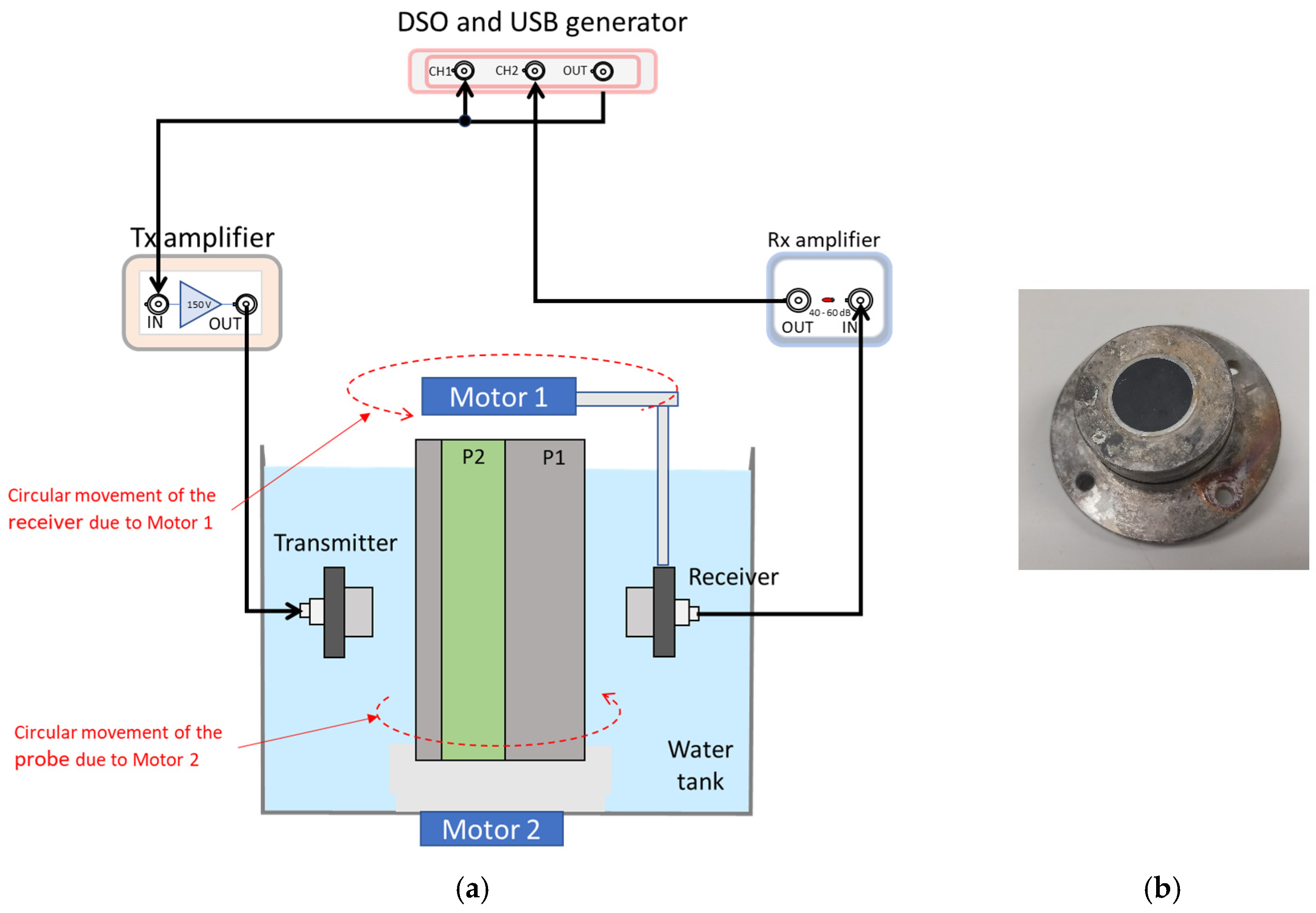
The setup for the measurements is shown in Figure 8a.

It contained the following elements:

• A Handyscope HS5 (TiePie, Sneek, The Netherlands)signal generator that acts as an acquirer and also as a generator of arbitrary functions.
• A FALCO WMA-300 (Falco Systems, Amsterdam, The Netherlands) transmission amplifier capable of generating voltages up to ±150 V, with a bandwidth from DC to 5 MHz.
• A 5660B pre-amplifier (Panametrics, Waltham MA, USA) reception amplifier, a low-noise amplifier with a wide bandwidth from 500 Hz to 40 MHz. The gain is selectable at 40 or 60 dB. In our case, we used the 40 dB setting.
• Motor 1 and motor 2 were used to move the probe and the receiving transducer, which were controlled by an Arduino system through a specific driver. Motor 1 and 2 were stepper motors with 200 steps per revolution (3A max).
• Olympus Immersion Transducer Power Series U8517179 (Olympus Europa SE & Co. KG, Hamburg, Germany) 1 MHz immersion transducers (see Figure 8b).

Immersion ultrasound coupling was used instead of airborne ultrasound because the ultrasound absorption factor is lower in water (0.0022 dB/cm/MHz) than in air (1.64 dB/cm/MHz) [29] as it is the reflection factor between the water–cement interface. However, this will favor the creation of multiple reflections due to the size of the tomography tank.

The transducers were excited by a burst signal, with five cycles, an amplitude of 150 V peak, and a central frequency of 1 MHz. Meanwhile, the sampling frequency was 50 MHz, with an average performed every 16 traces and a vertical resolution of 14 bits (originally 12 real bits, enhanced through averaging across traces).

In addition, as shown in Figure 8, the number of beams and the number of directions were controlled by motor 1 (M1) and motor 2 (M2), respectively. Motor 1 sweeps from 0° to 180° with a step of 3.6° (52 positions), where the receiver transducer is mounted, while motor 2 sweeps from 0° to 360° with a step of 5.25° (70 positions), controlling the rotation of the specimen (and the transmitter).

Therefore, for each specimen, a total of 3640 measurements were performed using 52 reception positions, with a step of 3.6°, and 70 transmission positions, with a step of 5.25°. Figure 9 presents a flowchart with pseudocode depicting the execution of the measurement process.

3.3. Simulation Measurements

For the training and test cases, we used the opensource k-Wave toolbox [30,31,32]. The model was based on the k-space pseudospectral time domain (PSTD) method to solve the nonlinear wave equation in a Cartesian coordinate system and simulate linear and nonlinear wave fields in fluid media [31,32]. This toolbox requires the properties of the computational grid, the medium properties, the source terms, and the reception points used to record the evolution of the wave field over time. For this work, 2D simulations were carried out; therefore, the spatial points were defined along the X and Y axes.

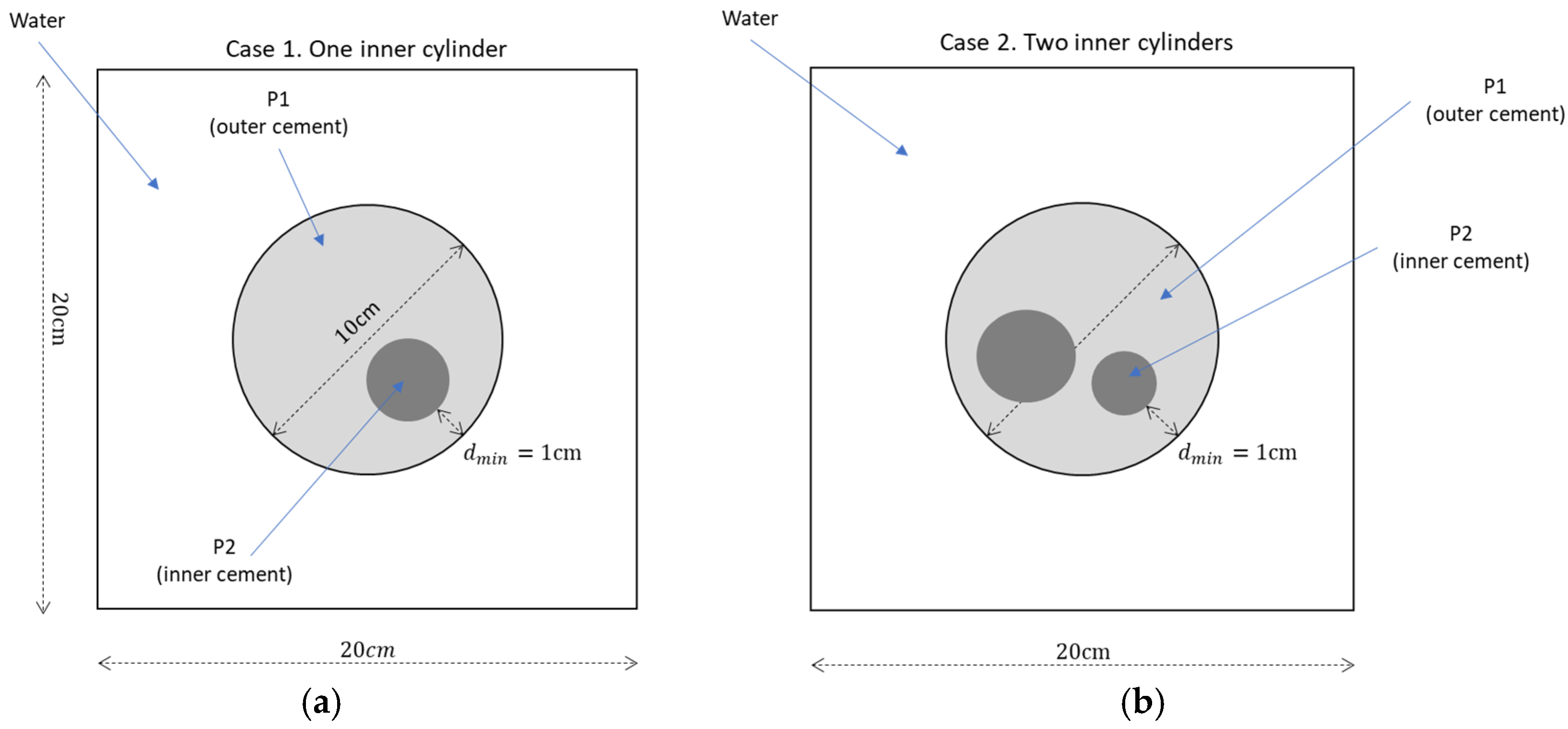
The grid size was defined using 600 × 600 grid points with Δx = Δy = 1/3 ${\displaystyle \frac{\mathrm{mm}}{\mathrm{point}}}$ resolution, resulting in a simulated area of 20 × 20 $\mathrm{c}{\mathrm{m}}^2$. The created sample corresponds to a concrete cylinder with a diameter of 10 cm in the center of the simulated area, called the outer cement or P1, which was surrounded by water. Inside of this cylinder, 1 or 2 additional cylinders of another type of cement were added (inner cement or P2). Moreover, the inner cylinders were of random sizes and placed in random positions, but some restrictions were applied: the diameters were uniformly distributed between 2 cm and 6 cm (U(2, 6) cm), there was a minimum distance of 1 cm between the edge of the inner cylinder(s) and the edge of the outer cylinder, and there were two possible cases (case 1 with only 1 inner cylinder and case 2 with 2 non-overlapping inner cylinders). An example of both cases is shown in Figure 10.

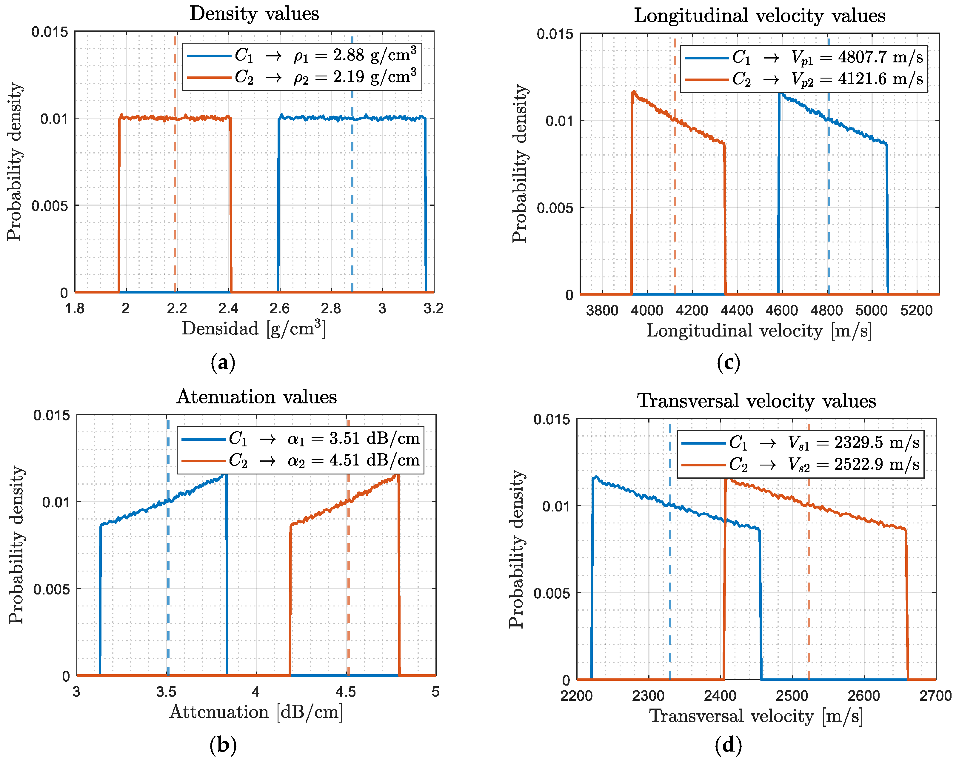
The primary characteristics of the parameters and materials used for simulation are summarized in Table 1. To better approximate the training process to real-world conditions, a uniform distribution of density values was assigned for both cement materials. Figure 11a illustrates the uniform density distribution with a range of ±10% relative to the central values: ${\rho }_1=2.88$ for the outer cement (P1) and ${\rho }_2=2.19$ for the inner cement (P2). The variations in the remaining parameters were derived from the changes in density and their respective distributions are depicted in Figure 11b–d. This approach is reflected in

Table 2. Range of values for the different parameters used in the simulation.

	Water	Outer Cement 1 (P1)			Inner Cement 2 (P2)
		Central	Range		Central	Range
$\mathrm{Density} \left(\rho \right)$$\left[{\displaystyle \frac{\mathrm{g}}{\mathrm{c}{\mathrm{m}}^3}}\right]$	1	2.88	2.59	3.17	2.19	1.97	2.41
$\mathrm{Longitudinal} \mathrm{velocity} \left(C_p\right)$$\left[{\displaystyle \frac{\mathrm{m}}{\mathrm{s}}}\right]$	1479.9	4807.7	5067.8	4584.0	4121.6	4344.5	3929.8
$\mathrm{Transversal} \mathrm{velocity} \left(C_s\right)$$\left[{\displaystyle \frac{\mathrm{m}}{\mathrm{s}}}\right]$	0	2522.9	2659.4	2405.5	2329.5	2455.5	2221.1
$\mathrm{Attenuation} \left(\alpha \right)$$\left[\mathrm{d}\mathrm{B}\right]$	0.00217	3.5	3.13	3.84	4.5	4.19	4.79
$\mathrm{Att}. \mathrm{power} \mathrm{coefficient} \left({\mathrm{\alpha }}_{\mathrm{power}}\right)$	2	0.9			0.9
$\mathrm{Diameter} \left[\mathrm{c}\mathrm{m}\right]$	-	10			4	2	6

, which presents the central values and the corresponding range for each parameter. It is also important to note that the parameters for water were kept constant. As a result, the water column in the table does not present a range; it only includes the fixed value applied across all the simulated cases.

For the simulation process, a through-transmission was selected where,

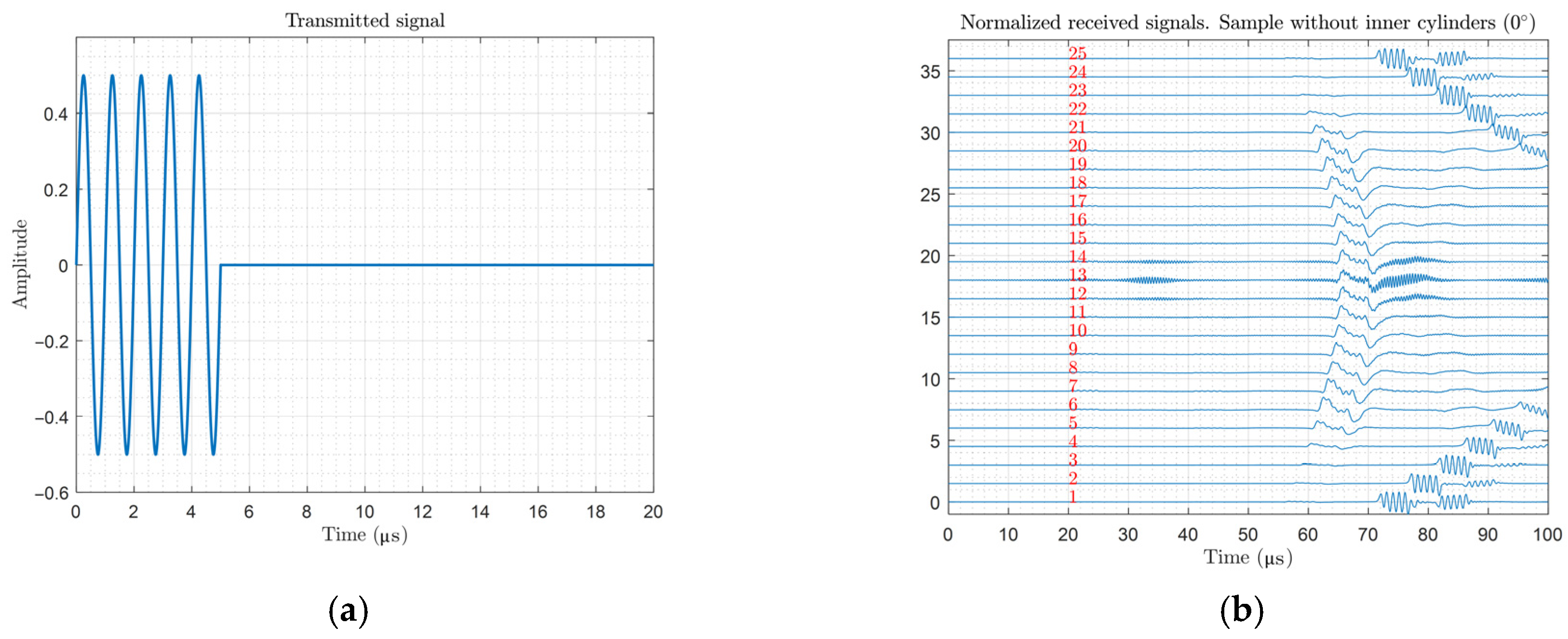
• The transmitted signal corresponded to a burst signal of 1 MHz and 5 cycles (Figure 12a). The end time was set to 100 μs and the sampling frequency was 100 MHz, yielding 10,000 points for each signal.
• There were 25 reception transducers, equally distributed from 0° to 180° and placed in front of the transmission transducer. The reception transducers received signals simultaneously; that is, for each signal transmitted, 25 signals were received (Figure 12b).
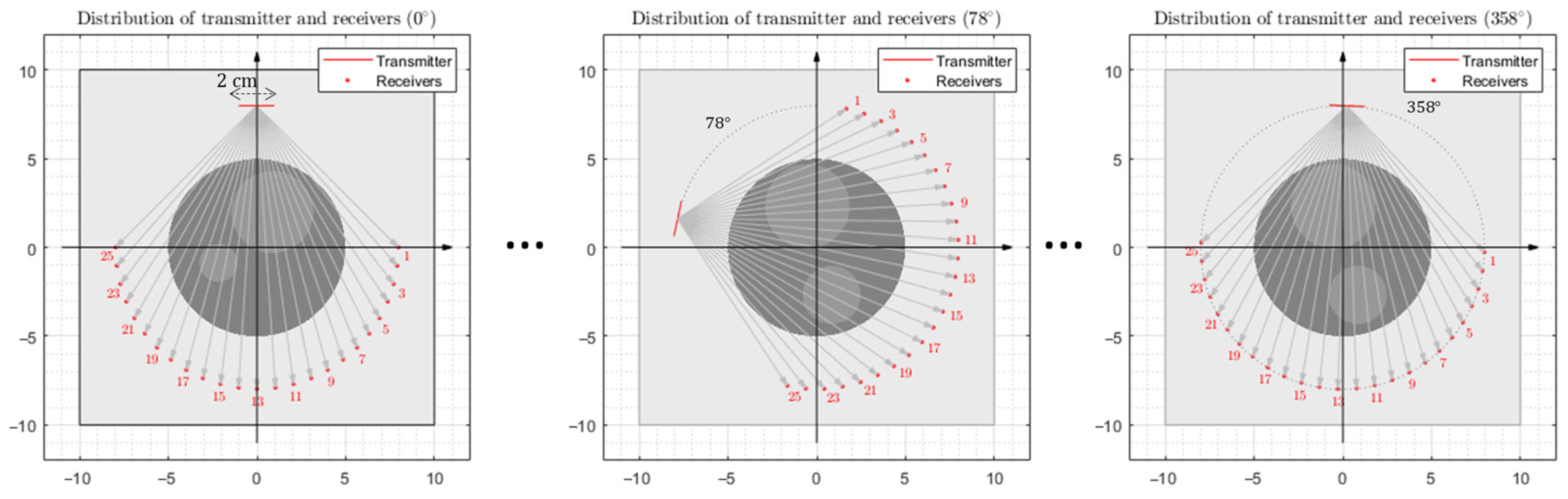
• The transmission transducer was a 2 cm active surface and was placed in water 3 cm from the outer cylinder (Figure 13).
• The whole set of transducers was rotated around the cement sample in 2-degree increments from 0° to 358° (Figure 13), resulting in 180 equally angularly distributed positions.

Therefore, each simulation was composed of 4500 signals: 180 transmission positions multiplied by 25 reception positions for each transmission position.

The simulations were carried out using a GPU GEFORCE RTX 2080 super and the simulation time for each case was about 1.58 h. A total of 146 cases were simulated, requiring around 9 days of simulation. Considering how the signals were obtained, each simulation/case was reused (data augmentation) to generate additional cases by rotating the original image and reordering the transmitted and received signals. Hence, from each simulation, an additional 180 cases were obtained through matrix rotation and signal reordering. In this way, the number of cases significantly increased from 146 cases to 26,280 cases with the minimum computational cost.

3.4. Parameters Extraction and Sinograms Obtention

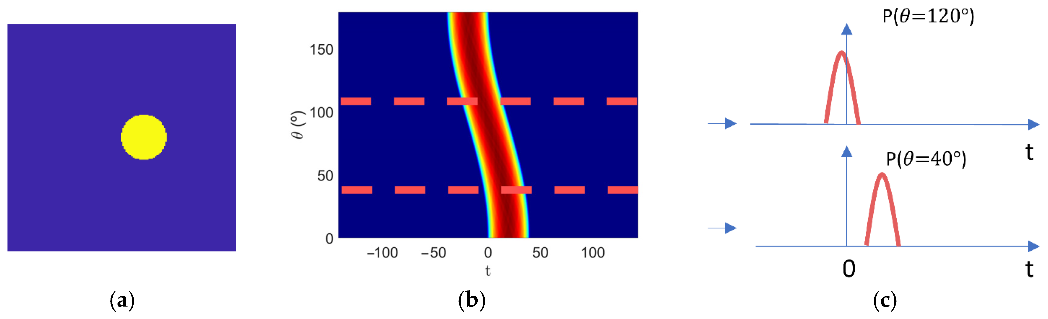
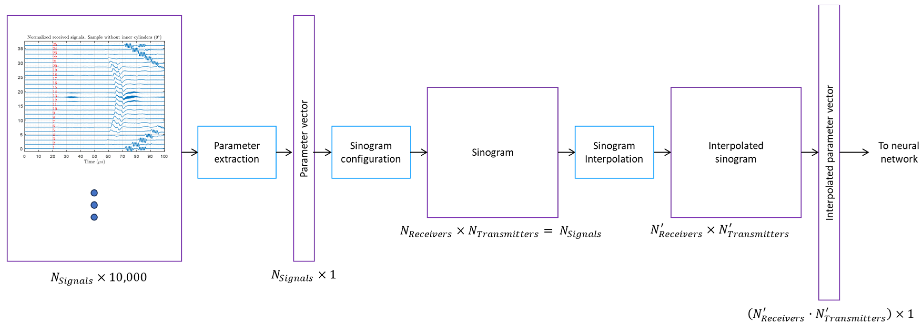
As described in Section 2.1, the sinogram is a two-dimensional representation in which the projections are placed according to the different directions through which the object is illuminated. As shown in Figure 14, for each obtained signal, a parameter estimation was applied [33]. In this work, the attenuation that the signal experienced with respect to the transmitted signal was obtained [34,35] (Equations (4)–(6)).

$${\alpha }_{ij}\left[{\displaystyle \frac{\mathrm{dB}}{\mathrm{cm}}}\right]={\displaystyle \frac{P_{tx,i}\left[\mathrm{dB}\right]-P_{rx,j}\left[\mathrm{dB}\right]+G\left[\mathrm{dB}\right]}{d_{ij}\left[\mathrm{cm}\right]}}$$

(4)

$$P_{tx,i}\left[\mathrm{dB}\right]=10·{\mathit{log}}_{10}\left({\displaystyle \frac{1}{N_{tx}}}\sum _{n=0}^{N_{tx}}{\left|x_{tx,i}\left[n\right]\right|}^2\right)$$

(5)

$$P_{rx,j}[\mathrm{dB}]=10·{\mathit{log}}_{10}\left({\displaystyle \frac{1}{N_{rx}}}\sum _{n=0}^{N_{rx}}{\left|x_{rx,j}\left[n\right]\right|}^2\right)$$

(6)

where

• $i$ represents the position of the transmitter ($i=[1,\dots ,180]$);
• $j$ represents the position of the receiver with respect to the position of the transmitter ($j=[1,\dots ,25]$);
• ${\mathrm{P}}_{\mathrm{tx},\mathrm{i}}\left[\mathrm{dB}\right]$ represents the power of the transmitted signal for position i. It is a constant value and it does not depend on i. ${\mathrm{x}}_{\mathrm{tx},\mathrm{i}}\left[\mathrm{n}\right]$ is the discrete transmitted signal;
• ${\mathrm{P}}_{\mathrm{rx},\mathrm{j}} \left[\mathrm{dB}\right]$ represents the power of the received signal for sensor $j$. It depends on the transmitter position, receiver position, and the properties and morphology of the sample. ${\mathrm{x}}_{\mathrm{rx},\mathrm{j}}\left[\mathrm{n}\right]$ is the discrete received signal;
• ${\mathrm{N}}_{\mathrm{tx}}$ and ${\mathrm{N}}_{\mathrm{rx}}$ are the number of transmitted and received signals, respectively. $N_{rx}$ was set to 7000 samples, corresponding to 70 μs, to prevent unwanted signals such as those from surface propagation and/or reflections from the container walls;
• ${\mathrm{d}}_{\mathrm{ij}}$ [cm] is the distance between the transmitter and the receiver;
• $G \left[\mathrm{dB}\right]$ represents the gain of the amplifier used. In this work and for the real measurements, its value was fixed at $40 \mathrm{d}\mathrm{B}$;

In this work, the columns of the sinogram correspond to the rotation angle of the transmitter, while the rows correspond to the position of the receivers. Each position of this matrix contains the value of the attenuation parameter extracted for that specific measurement. The sinogram is then converted into a column vector that will feed the neural network, either for training or for testing. It is important to notice that, although the reconstruction of the sinogram from the parameters of each signal is not necessary because the neural network does not require it, it is important to readjust/synchronize the size of the sinograms between the real measurements and simulated ones (see Figure 14). The sinogram interpolation module readjusts the size of the sinogram to have the same dimensions as the simulated sinograms and the real signals. The interpolation process is a cubic interpolation between adjacent samples (Figure 14).

3.5. Neural Networks: Implemented Models

As explained in Section 2.2. Neural Networks the objective was to perform tomographic reconstruction using ultrasonic projections; the inputs are the obtained projections (sinograms), while the outputs are the reconstructed images associated with their projections (Figure 4).

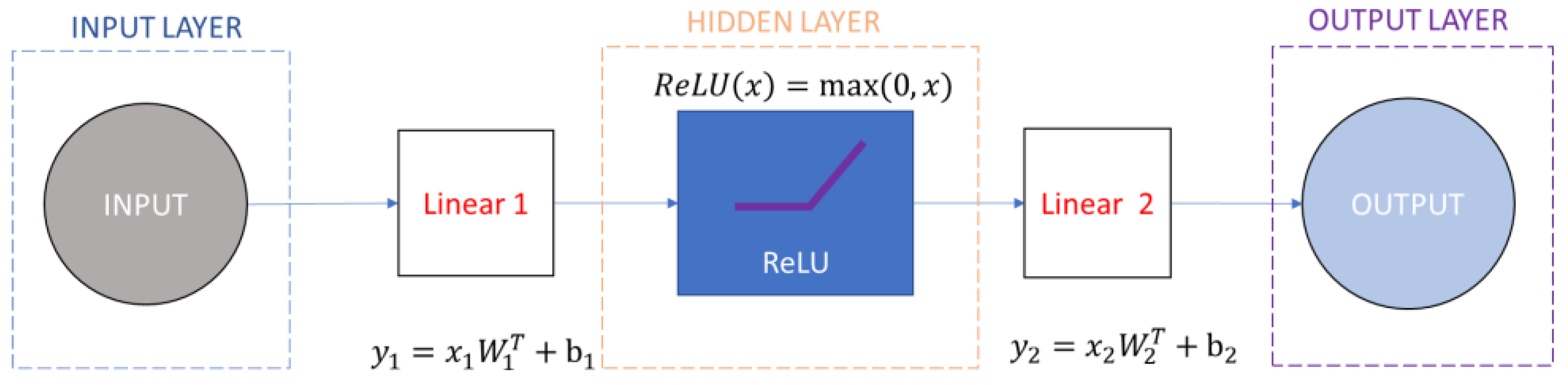
Two neural network models were proposed in this study. The first model was designed for pure reconstruction purposes (Figure 15), where the pixel values correspond to the selected parameter for the reconstruction such as speed. This is a regression problem. The models were implemented using the Pytorch^® framework [36].

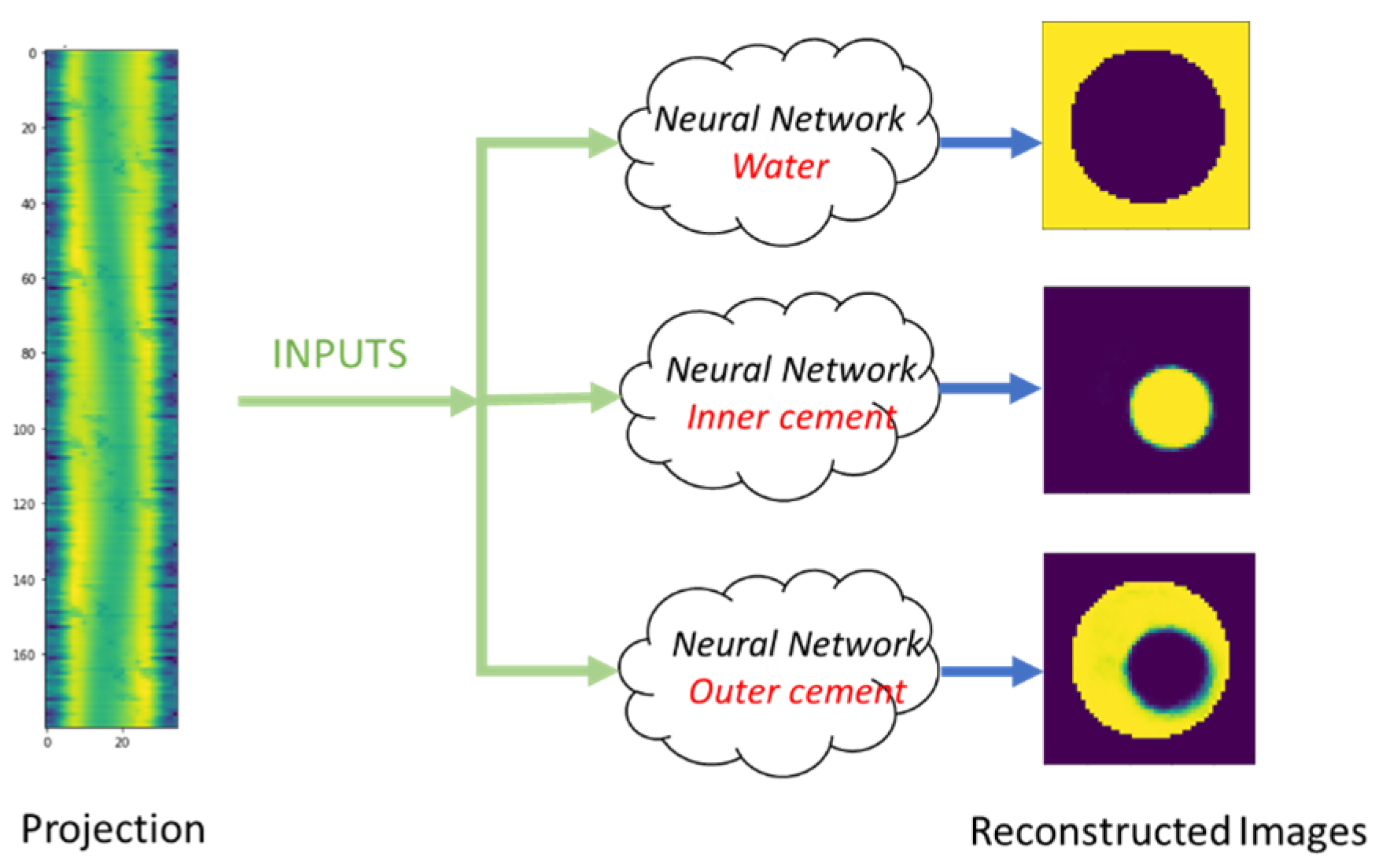
The second model functions as a classifier, where the number of classes corresponds to the materials to be identified in the projections. Moreover, the output of this network consists of active pixels corresponding to the material being analyzed. If the specimen under investigation is composed of three distinct materials, three separate neural networks will be employed, each one trained to identify a specific material. Both models share the same input (Figure 16), but this second model will correspond to a classification problem. As a classification problem, the neural network must assign each pixel of the reconstructed image to one of the three possible material types (water, P1, or P2).

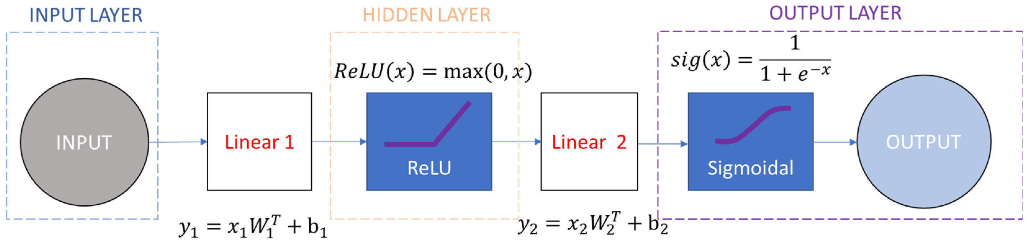
The following model for locating and classifying the materials to be reconstructed is the same as the previous one, but with the addition of a sigmoidal activation function before the output (Figure 17). In this sense, the main difference is that the sigmoidal activation function helps to binarize the image pixel values.

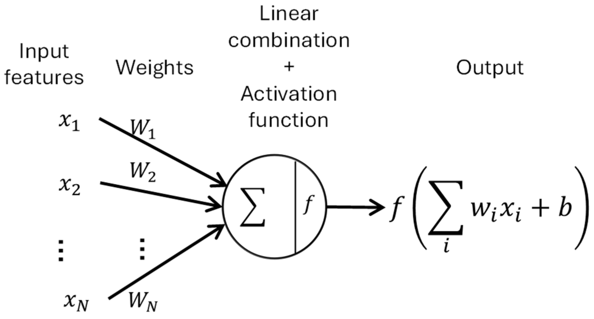
Both models use a ReLU (Rectified Linear Unit) activation function for the intermediate layer, which can accelerate the training process since the derivative of this function is for positive inputs. Due to this constant derivative, additional computation time for error terms during training is not required. Moreover, ReLU is widely used to identify nonlinear relationships between inputs and outputs, as well as in cases where the outputs are continuous, as discussed in this study.

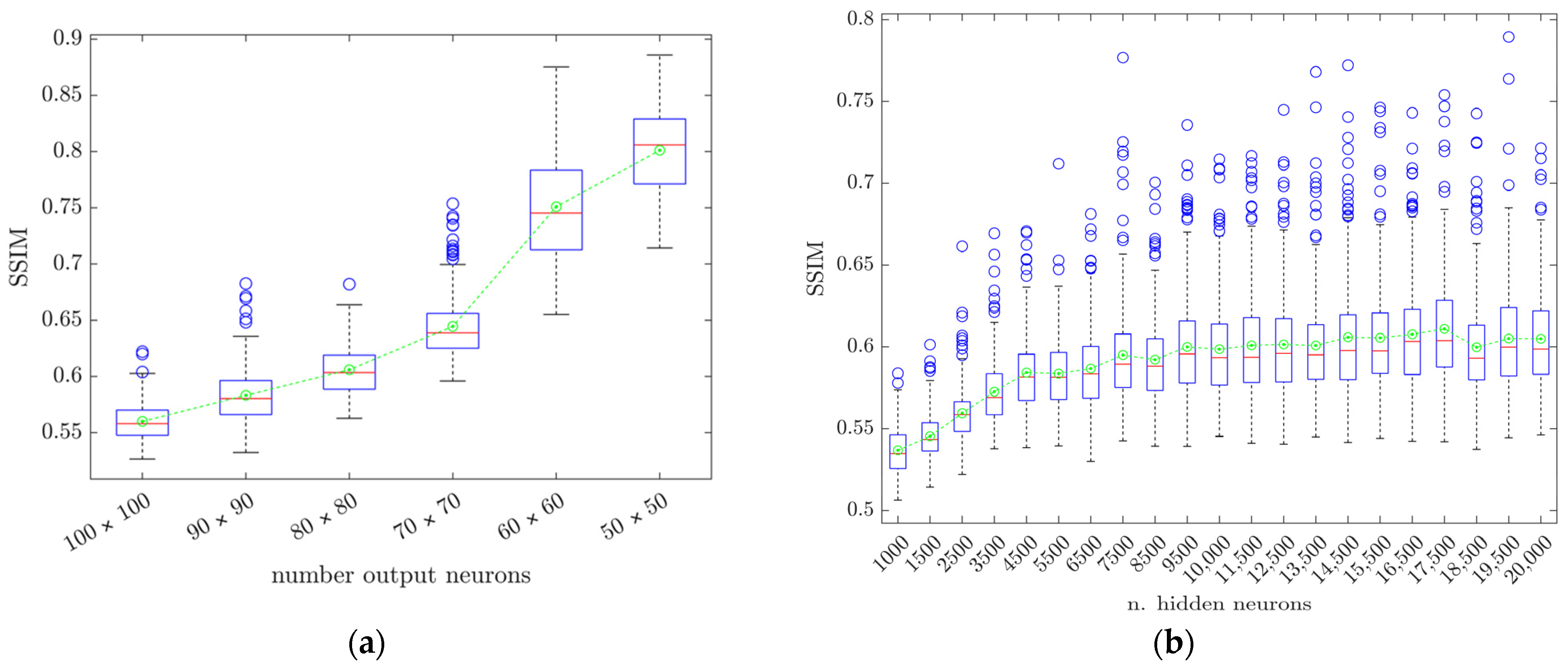
3.6. Optimization of Neural Network Parameters

As the two neural network models are practically the same, only one was studied for parameters optimization. The dimensions of the input layer depend on the dimensions of the sinogram (number of transmitters and receivers) from the simulations or real cases and are, therefore, limited for the study of their variations. However, we can study the variation in the number of output and hidden neurons, as well as the number of hidden layers, and find the best configuration of hyperparameters for the dataset we used. We studied three variations: the number of output neurons (2500 to 10,000), hidden neurons (10,000 to 20,000), and hidden layers (1 to 4).

To evaluate the quality of the reconstruction, we use the Structural Similarity Index (SSIM) parameter [31] that measures the similarity between two images according to Equation (7):

$$SSIM\left(x,y\right)={\displaystyle \frac{\left({\mu }_x^2+{\mu }_y^2+C_1\right)\left({\sigma }_x^2+{\sigma }_y^2+C_2\right)}{\left(2{\mu }_x{\mu }_y+C_1\right)\left(2{\sigma }_{xy}+C_2\right)}},$$

(7)

where $x$ and $y$ are the row images being compared, ${\mu }_x$ and ${\mu }_y$ are the mean values of the images, ${\sigma }_x^2$ and ${\sigma }_y^2$ are their variances, ${\sigma }_{xy}$ is the covariance between $x$ and $y$, and $C_1$ and $C_2$ are small constants to avoid division by zero. The metric is calculated between two images $x$ and $y$ and the value falls between 0 (low similarity) and 1 (perfect similarity) for images with non-negative pixel values.

Regarding the dataset for this optimization study, we split the 3760 images, a part of the simulated dataset, as follows: 60% for training, 26% for validation, and 14% for testing. The random seed was maintained between variation studies. In this way, the variations in each parameter were comparable with each other. The results are presented in

Table 3. Result of optimization parameters for neural network model.

Neurons in input layer	6300
Neurons in hidden layer	2500
Neurons in output layer	2500
Number of hidden layers	1
Batch size	10
Initial learning rate	0.9

and the model used these values for the reconstruction evaluation with simulation and real cases. For more details about the process used to obtain these parameters, see Appendix A.1 in Appendix A.

4. Results

After optimizing the parameters for the neural network training, the reconstruction performance of the two models (regression and classification) were evaluated. It is important to note that, in both cases, the training cases were extracted from the simulated dataset, as it contains the largest number of samples. Specifically, the simulated dataset comprises 146 original cases, which expand to 26,280 cases through data augmentation, whereas the dataset based on real measurements only contains four cases.

The number of cases of the datasets and the number of cases for the training and testing are presented in

Table 4. Number of elements in each dataset.

Dataset	Number of Elements
	Total	Training	Validation	Testing
Simulated	26,280	14,280	6000	6000
Real	4	-	-	4

.

The behavior of the two models (regression and classification) was evaluated using projections obtained by attenuation through the integration of the whole temporal signal squared, divided by the distance travelled by each beam formed by the transmitter and receiver. In the following sections, the results obtained for the simulated sinograms and real sinograms will be presented.

4.1. Simulated Sinograms: Physical Parameter Estimation (Model 1)

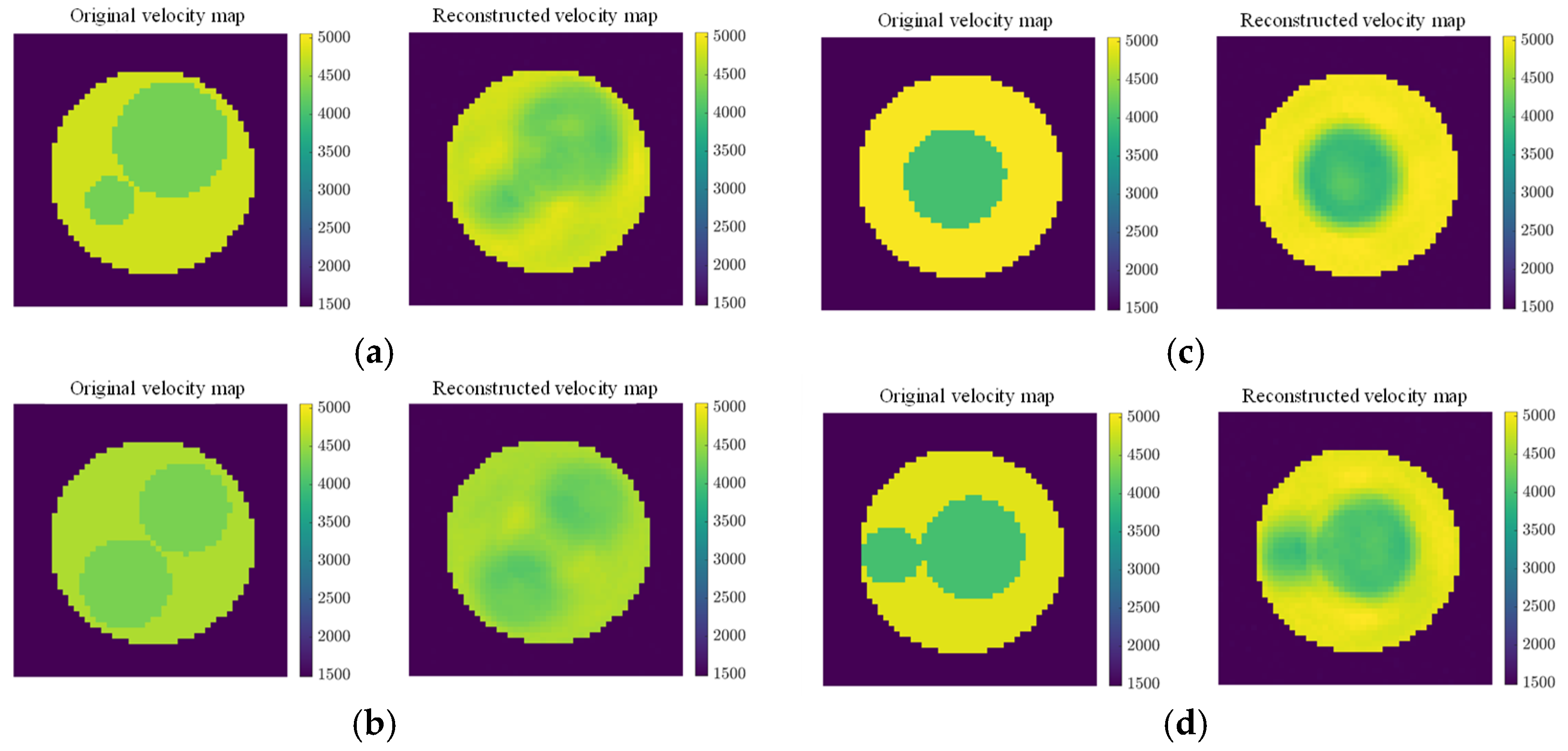
The objective of this model was to estimate the longitudinal velocities inside of the specimens (regression problem). It should be noted that, in the simulations, the densities and velocities of the cements followed a uniform distribution. Specifically, the velocity of the external cement (P1) ranged between 4585 m/s and 5056.24 m/s, while the internal cement (P2) ranged between 3934.76 m/s and 4335.79 m/s.

Figure 18 presents four selected cases where the left images correspond to the original sample with its actual velocity map and the right images represent the reconstructed velocity map. In this sense, a good estimation of both the velocity values and the morphology of the internal cement structures can be observed. Since it is not feasible to display all 6000 cases, Figure 19a illustrates the SSIM values for the entire testing dataset. The SSIM metric ranged from 0 (completely different images) to 1 (identical images) and accounts for the similarities in both the numerical values and the morphology. As shown, the mean SSIM value exceeded 0.95, with low variance, indicating a high-quality reconstruction.

As observed in Figure 18, when the longitudinal wave velocity of the outer cement (P1) and inner cement (P2) became more similar, the network encountered greater difficulties in performing the reconstructions (Figure 18a,b). Conversely, as the difference increased, the outlines of the internal objects became sharper, leading to improved reconstruction accuracy (Figure 18c,d).

Additionally, the blurring effect observed at material boundaries is an intrinsic characteristic of this model and was more pronounced due to the need to estimate continuous values. In contrast, the classification model described in the following section was designed to distinguish between different material types. As a result, the range of possible values was more constrained as it employs a sigmoid activation function, which exhibits a steeper derivative compared to the linear activation function used in the regression model. This sharper transition in the classification model reduces boundary blurring compared to the regression approach.

4.2. Simulated Sinograms: Material Classification (Model 2)

This second model focuses on detecting different types of cement instead of estimating material properties such as velocity. In other words, it reconstructs binary images that indicate the presence or absence of each material. To achieve this, a classification model was proposed in which three networks were trained, each specializing in one of the three available materials: water, outer cement, and inner cement (see Figure 16 and Figure 17). During the training process, the reference image corresponds to the binarized image for the target material and the SSIM parameter is used as the quality metric. In this case, since the SSIM between the binarized reference image and the reconstructed image for each material is computed, three SSIM values are obtained, one for each material (water, outer cement (P1), and inner cement (P2)).

In the water-specific reconstruction model, the SSIM approached 1 due to the absence of variation in both the velocity of water, which remained constant at 1479.9 m/s, and its spatial distribution. Consequently, the neural network learned to consistently identify this region as water, regardless of the sinograms.

Figure 20 presents two selected cases using the cement reconstruction models where the left images correspond to the original image with the classified material (water, outer cement, and inner cement), while the right images represent the reconstructed image for cement P1 and cement P2. The probability scores for these images ranged between 0 (zero probability of this material) and 1 (one hundred percent probability of this material). It can be observed that the probability remained close to 1 for each material. As expected, the boundaries between P1 and P2 were diffuse, and the probability fluctuated between 0 and 1. The SSIM values exceeded 0.95 for both materials, indicating a high-quality reconstruction. For this case, we had two SSIM values: one for the P1 material reconstruction and one for the P2 material reconstruction.

4.3. Real Sinograms: Material Classification (Model 2)

The quality of the results obtained from the real measurements did not match those from the simulations. This difference was influenced by various factors that affect reconstruction quality but were not present during the simulation process:

• The signal-to-noise relationship due to the signals is real and is affected by interference, electronic noise, and noise from the amplifiers.
• Small dispersers that were not considered in the simulation.
• Multiple reflections due to the placement of the transducers inside the water vessel as well as their walls.

These aspects produced discrepancies between the sinograms acquired empirically and those derived from the simulations, resulting in a worse reconstruction performance than that obtained with the simulations. However, since we were interested in seeing the transition of the carbonation front, we used model 2 (classification) for the detection of the internal cement (P2). Therefore, the neural network trained with simulations was employed to reconstruct the internal cement (P2) from real sinograms. 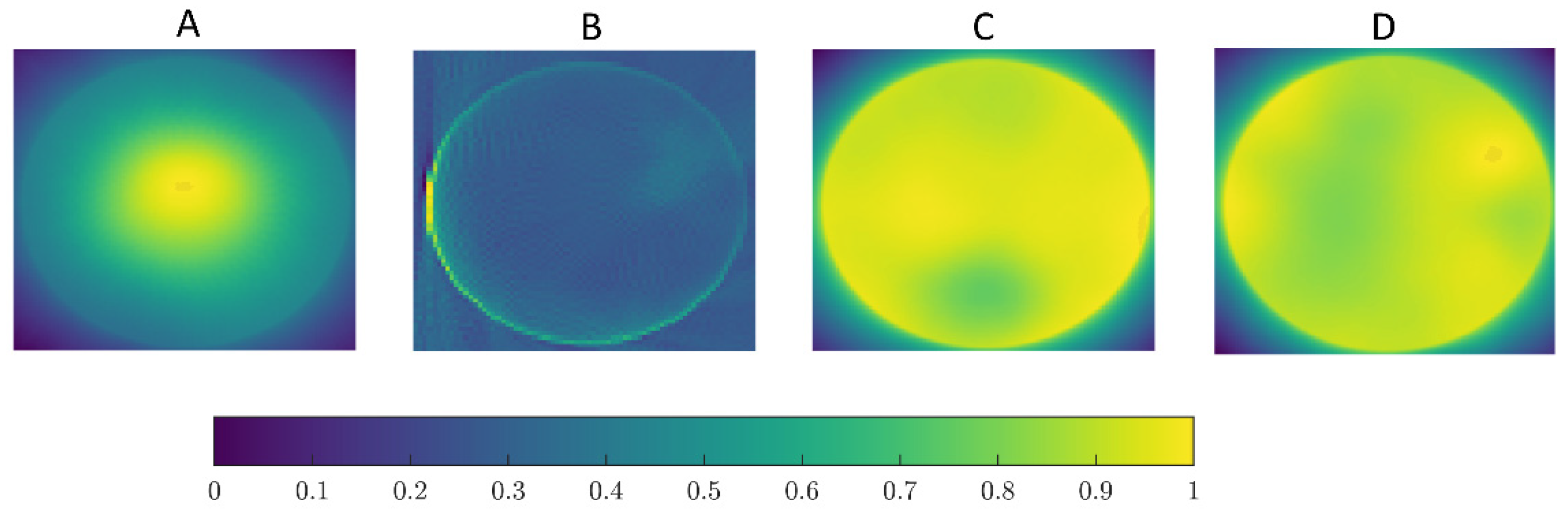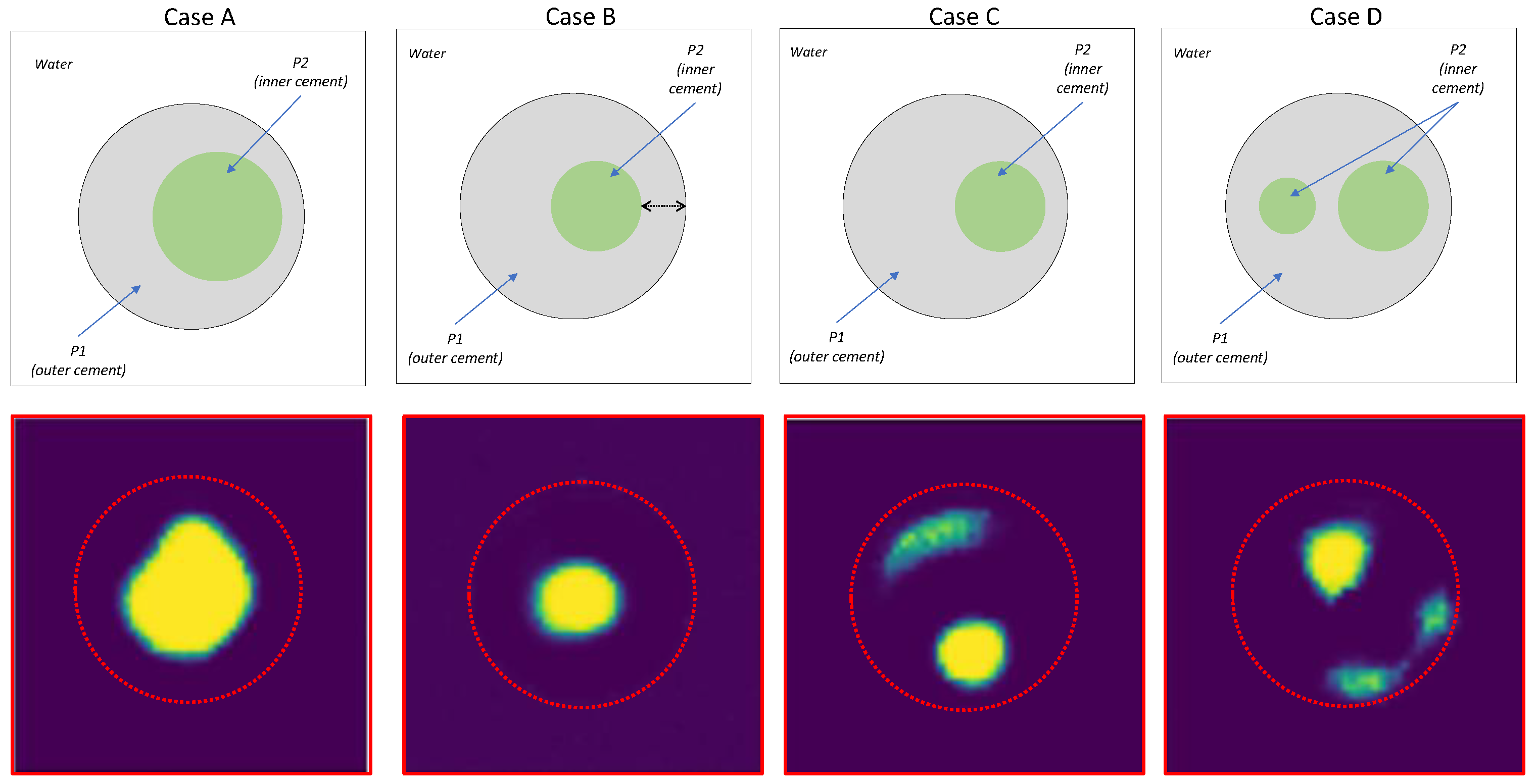Figure 21 shows the real reconstructions of the P2 for the different real cases.

In the reconstruction of cases with a single internal element, the model performed well. However, some deformation was observed such as the flattening of objects that were theoretically circular (Figure 21, cases A and B). Despite this, the effect was not significant, and the overall shape of the object was preserved. In cases with two internal objects, the reconstruction of one object failed and artifacts appeared (Figure 21 case D). Furthermore, these artifacts were also observed in case C and were likely due to the low signal-to-noise ratio in the sinograms or offset errors in the measurement system. Such artifacts could potentially lead to the misidentification of additional internal elements in real-world scenarios where none exists.

Table 5. Quality metrics for reconstruction in real cases using the trained model 2.

Case	SSIM
A	0.82
B	0.70
C	0.72
D	0.61

presents the SSIM values, which correlate with the descriptive analysis provided.

A comparison of the traditional reconstruction methods using the real measure was made and can be seen in

Table A1. Comparison of the main conventional reconstruction algorithms with the proposed model.

Specimen	Conventional Reconstruction Algorithms								Proposed Model
	FBP	DFT	ART	CART	SART	SIRT	MLP-BPE	RBFNN
A	0.421	0.132	0.132	0.159	0.384	0.361	0.256	0.322	0.820
B	0.441	0.156	0.442	0.465	0.315	0.281	0.181	0.465	0.700
C	0.512	0.221	0.359	0.238	0.295	0.284	0.327	0.317	0.720
D	0.507	0.160	0.378	0.240	0.256	0.262	0.294	0.252	0.610
Mean	0.470	0.167	0.328	0.276	0.313	0.297	0.265	0.339	0.713
SD	0.036	0.029	0.105	0.102	0.042	0.034	0.049	0.070	0.067

; the reconstruction images for each method and specimen are shown in Figure A3 and Figure A4 in Appendix A.2 of Appendix A.

The proposed model demonstrated superiority to conventional algorithms in terms of SSIM, as evidenced by the mean SSIM value of 0.714 (±0.067) across the four real cases for each reconstruction method, which is significantly higher than the mean SSIM value of 0.470 (±0.036) for the conventional algorithms.

5. Discussion and Conclusions

This study explored the application of neural networks for ultrasound tomographic reconstruction of cementitious materials, particularly in the context of gradient damage assessments. The proposed approach leverages simulated training data to overcome the challenges associated with acquiring large real-world datasets, both in terms of cost and time. The ability to generate simulated datasets at a reduced economic and computational cost enables the creation of large, well-controlled datasets, facilitating complex training processes.

Two neural network models were developed: a regression-based model for estimating material properties and a classification model for identifying different cement types. The results obtained from the simulations demonstrated high reconstruction accuracy, with Structural Similarity Index (SSIM) values exceeding 0.95, indicating strong performance for both models. These models effectively differentiated between materials, with well-defined boundaries when the contrast in acoustic properties was sufficient. With real cases, model 2 (classifier model) achieved superior performance in comparison to all the conventional tomographic reconstruction models in detecting the inner material. In the regression problem, the SSIM did not reach values (0.82) as high as in the classification problem (0.95), where the reconstruction of the material boundaries was significantly affected by a pronounced blurring effect. This undesired effect is an intrinsic effect of the problem itself because the activation function must be a linear activation function with a derivative lower than the sigmoidal activation function.

When applied to real measurement data, the neural network maintained its effectiveness in cases with a single internal element. Although single-object cases are the least demanding scenario, traditional methods present problems when reconstructing them. This fact demonstrates the advantage of our approach over traditional tomographic reconstruction algorithms. In fact, compared with the traditional algorithms, the classification model achieved a better mean SSIM for the four specimens (0.713 ± 0.067). 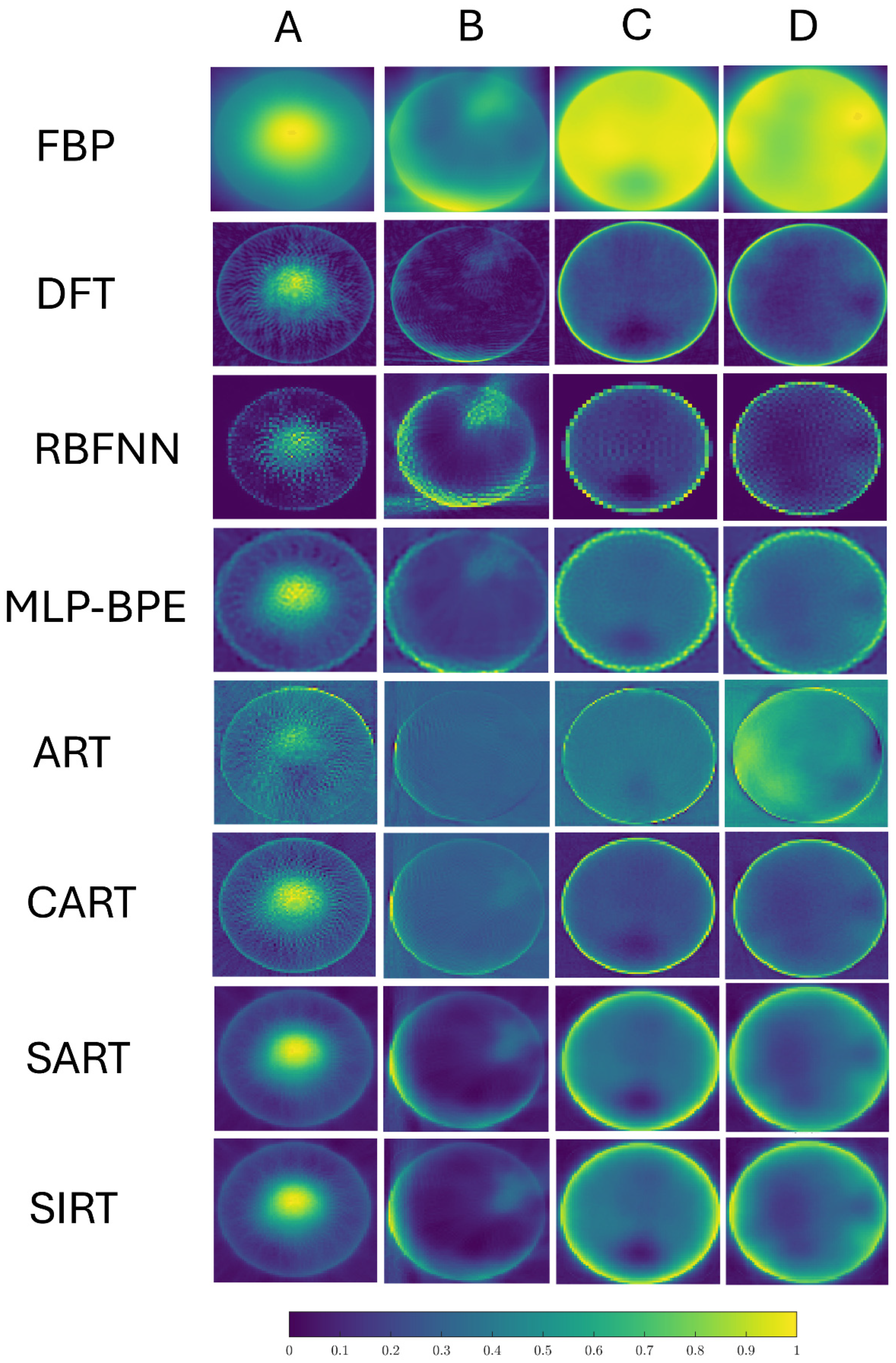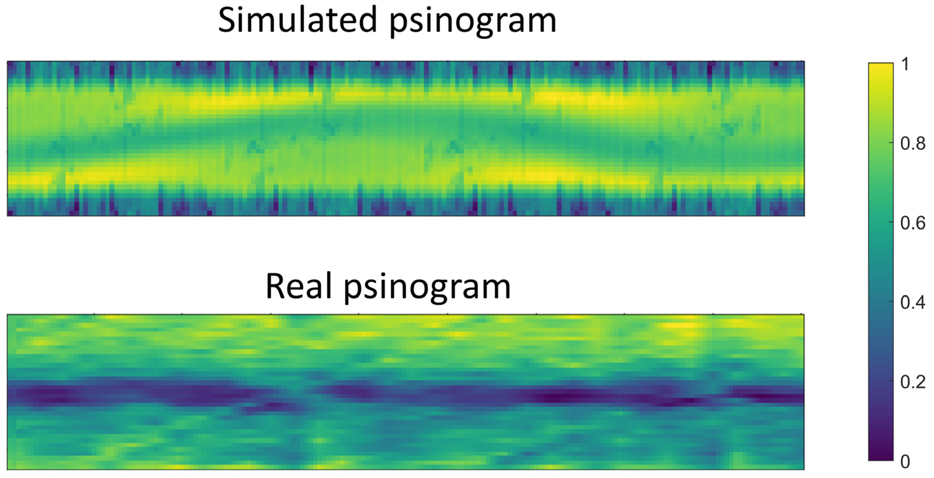Furthermore, the presence of multiple internal structures led to the reconstruction of artifacts and occasional misidentifications, primarily due to discrepancies between the real and simulated sinograms (see Figure 22), the low signal-to-noise ratios, and measurement system offsets. These discrepancies between the simulated and real data were attributed to the limitations of simulations to replicate all the processes that occur in reality. Nevertheless, the models’ performance in the experiments that required a high investment of time and financial resources was remarkable. In addition, they allowed for experimentation with variables in a controlled environment. Finally, the use of these models can facilitate the creation of deep learning prototypes before training with real data.

Despite these limitations, the model successfully captured the general morphology of internal structures, proving the feasibility of training a simple neural network using simulated data. The simplicity of the neural network together with the low variability represented in the simulation cases is likely to limit the performance of the model in demanding chaos. However, due to its simplicity, it can be easily implemented with embedded systems or low specification hardware and can be used for detecting a specific damage gradient. It is understood that the existence of a greater number of simulated cases of a higher quality (i.e., closer to reality) would facilitate the use of more complex neural models. In the domain of image reconstruction, convolutional autoencoders have demonstrated notable efficacy. However, it should be noted that these architectures are more data-hungry and require more computational power (usually GPU-accelerated). In practice, as already mentioned, more challenging cases may appear. Thus, further research is necessary, and there are several research directions that can be taken to enhance model performance. Future research should focus on creating more complex cases, such as air voids, reinforcement bars, and materials with scatterers of a certain size (i.e., aggregates) could be included to improve the reconstruction, as well as the use of more complex morphologies of the embedded materials, along with more complex simulations including noise (to evaluate the robustness of the reconstruction). Our current model could be used as a tool for labeling new cases and training a more complex model to achieve further generalization. Additionally, a few real cases should be added in the training of the model. The use of GANs as well as a parametric optimization of the simulation model variables (material properties) could decrease the difference between simulated and real data and improve the results of the reconstruction model. Moreover, the inclination of the transducers to have an oblique incidence and look for the excitation of surface waves could help to find answers on the damaged front.

Enhancing the measurement system and feature extraction (i.e., frequency-dependent attenuation or slowness), reducing noise (i.e., filtering), and incorporating advanced neural architectures such as convolutional networks, autoencoders (with multidimensional input sinograms), or convolutional autoencoder could further improve the reconstruction accuracy. Additionally, applying this methodology to practical cases, such as carbonation front detection in concrete, could provide valuable insights for structural health monitoring in civil engineering applications where the early detection of material degradation could prevent costly repairs and enhance infrastructure safety.