Abstract
In order to address the problems of in-plane rotation and fast motion during near-infrared (NIR) video target tracking, this study explores the application of capsule networks in NIR video and proposes a capsule network method based on background information and spectral position prediction. First, the history frame background information extraction module is proposed. This module performs spectral matching on the history frame images through the average spectral curve of the groundtruth value of the target and makes a rough distinction between the target and the background. On this basis, the background information of history frames is stored as a background pool for subsequent operations. The proposed background target routing module combines the traditional capsule network algorithm with spectral information. Specifically, the similarity between the target capsule and the background capsule in the spectral feature space is calculated, and the capsule weight allocation mechanism is dynamically adjusted. Thus, the discriminative ability of the target and background is strengthened. Finally, the spectral information position prediction module locates the center of the search region in the next frame by fusing the position information and spectral features of adjacent frames with the current frame. This module effectively reduces the computational complexity of feature extraction by capsule networks and improves tracking stability. Experimental evaluations demonstrate that the novel framework achieves superior performance compared to current methods, attaining a 70.3% success rate and 88.4% accuracy on near-infrared (NIR) data. Meanwhile, for visible spectrum (VIS) data analysis, the architecture maintains competitive effectiveness with a 59.6% success rate and 78.8% precision.
1. Introduction
Object tracking [1,2,3,4] refers to the technology of continuously locating and tracking a specific target in a video sequence, enabling the determination of its spatial coordinates and dynamic attributes across varying temporal segments. Its main task is to accurately track the target in dynamic scenes, especially when the target is blocked, the lighting changes [5], or the background is complex [6]. This technology holds significant prominence in computer vision [7,8] and is widely used in monitoring systems [9], autonomous driving [10], drone navigation [11], medical imaging [12], and other fields.
However, traditional visible light target tracking [13,14,15,16] technology faces many challenges in practical applications. Since the visible light band (VIS) is greatly affected by lighting conditions, the tracking effect of targets in weak light, complex backgrounds, or occlusion is often not ideal, which seriously limits the application scenarios of target tracking technology. These limitations have led to the application of hyperspectral imaging technology for target tracking [17,18].
Hyperspectral images (HSI) [19,20] are three-dimensional data cubes collected by hyperspectral cameras, which can capture image data in multiple bands of the electromagnetic spectrum, usually covering visible light [21,22,23], NIR [24,25,26], short-wave infrared [27], and other ranges. Each pixel has a complete spectral curve, which reflects the spectral characteristics of the material. The complete spectral curve associated with each pixel represents the inherent spectral characteristics of the material.
Among them, the near-infrared band (NIR) [28] generally refers to the electromagnetic spectrum with a wavelength range of about 700 nm to 2500 nm [29]. This band is between the red light end of visible light (about 700 nm) and the mid-infrared band (about 2500 nm). Compared with the visible light band, the NIR has a stronger penetration ability and can capture clear images in haze [30], low light [31], or even completely dark environments. In addition, the NIR has a higher degree of differentiation in the reflective characteristics of different materials and objects, making the segmentation and identification of targets in complex scenes more accurate. The spectral characteristics of near-infrared hyperspectral images (NIR-HSI) are relatively stable and less affected by changes in illumination. This consistency in spectral characteristics, even under varying illumination conditions, enhances the stability and reliability of target tracking. Therefore, NIR-HSI has demonstrated substantial importance in computer vision applications.
On the other hand, deep learning [32,33], especially convolutional neural networks (CNN) [34,35], has had a profound impact on target tracking technology. Traditional target tracking methods rely on manually designed features, such as color or texture, which are unstable in different scenarios. CNNs are able to learn and capture features at multiple levels [36], from simple edges to more abstract semantic content. They have stronger representational power, making the tracking algorithm more adaptable to complex situations such as lighting changes, target deformation, and occlusion [37]. In addition, the end-to-end learning paradigm in deep learning [38,39] enables direct regression from pixel data to positional predictions in tracking systems, mitigating cumulative inaccuracies caused by fragmented processing stages.
This study utilizes a capsule network as the feature extraction network. A capsule network [40,41] represents an emerging neural architecture designed to overcome the shortcomings of traditional CNNs in capturing spatial hierarchical information and processing complex deformations. To address this challenge, capsule networks have gained increasing adoption in algorithmic frameworks. M. E. Paoletti et al. [42] demonstrated their effectiveness in hyperspectral target classification tasks. Z. Mei et al. [43] improved on this by designing a capsule residual structure. Ma et al. [44] designed a pyramid dense capsule network for tracking purposes. In summary, these studies exhibit limitations in addressing complex target deformations, depth of feature extraction, and real-time performance. This research employs a capsule network framework to develop a near-infrared hyperspectral tracking system, integrating historical contextual analysis and spectral locational forecasting. The principal innovations of our methodology are summarized below:
- We propose a historical frame background extraction module (HFBE) to overcome the complex background in NIR hyperspectral target tracking. This module uses spectral information from different historical frames to construct background template features. A mask is generated by averaging spectral data from adjacent areas surrounding the target, enabling coarse separation between the target and background.
- A background target routing algorithm (BT) is proposed, which combines traditional capsule network algorithms with spectral information from target and background capsules. By computing feature correlations between foreground-background capsule pairs, the framework dynamically increases the weights of capsules with the same features as the background representation. After generating the background response map, the inverse is taken to get the target response map, thus achieving target localization.
- A spectral information position prediction module (SIP) is designed to determine the search area for the next frame. By integrating the spectral data of adjacent frames and the current prediction data, the spectral changes of the target can be dynamically adapted to improve the robustness of tracking.
This paper is divided into five components: Section 2 reviews critical developments in hyperspectral target detection literature. Section 3 details the architecture and implementation mechanisms of the proposed NIR spectral tracker. Section 4 evaluates algorithmic performance across benchmark hyperspectral datasets, including NIR spectral scenarios. Section 5 synthesizes key findings and outlines potential research extensions.
2. Related Work
2.1. Visual Object Tracking
Recent advances in visual object tracking have seen a shift from region proposal-based frameworks to more streamlined and end-to-end architectures. SiamCAR [45] proposes a fully convolutional Siamese network that formulates tracking as a pixel-wise classification and regression task, eliminating the need for region proposals and anchor boxes. Similarly, SiamBAN [15] extends this idea by integrating classification and regression into a unified fully convolutional network, enabling direct bounding box estimation without predefined anchors or multi-scale strategies. SiamGAT [46] further enhances the Siamese paradigm by introducing a graph attention mechanism that establishes part-to-part correspondence between the target and search regions, addressing the limitations of conventional cross-correlation methods. Moving beyond correlation-based fusion, TransT [1] replaces traditional correlation with attention-based modules, allowing for more effective feature interaction between the template and the search region. This attention-driven design mitigates the loss of semantic information and overcomes the limitations of local matching. In a similar spirit, STARK [47] adopts an encoder–decoder transformer architecture to directly predict bounding boxes in an end-to-end manner. It discards proposal generation and post-processing operations, achieving both high accuracy and real-time performance across various challenging benchmarks.
2.2. Capsule Network
Within the domain of NIR target tracking, the selection of features is important [48,49]. These features not only describe multiple attributes of the target object, such as shape and texture, but also they are related to the precision and stability of the tracking process. To further improve the tracking performance, capsule features [42] show their unique advantages. Capsule features not only capture the features of the object, but also emphasise the mutual and dependency relationships between different layers of capsules. However, traditional capsule networks focus on the capture of spatial features and ignore spectral information when extracting features. Spectral information, as unique to NIR [30] imaging technology, contains rich material clues that are conducive to accurate identification and tracking of targets. Therefore, by fusing spectral information with capsule features, the characteristics of the target object can be comprehensively depicted and provide a richer and more reliable basis for predicting the target location. This fusion strategy is expected to significantly enhance the performance of NIR target tracking systems.
The capsule network architecture comprises a dual-component framework: an encoder-decoder structure. The encoder incorporates sequential feature transformation stages, including convolutional operations for low-level feature extraction, primary capsule formation via initialization layers, and hierarchical capsule transformations through dynamic routing mechanisms. Conversely, the decoder implements a reconstruction module containing three-tier fully connected layers for dimensional mapping. Crucially, the network employs dynamic routing algorithms to propagate capsule activations between hierarchical levels, establishing iterative agreement processes that ensure context-aware feature propagation from lower to higher capsule tiers. The dynamic routing protocol is as follows: The feature vector is subjected to a squashing operation such that its length is between 0 and 1. The squashing function [40] is denoted as:
where denote the output produced by capsule j, represent its total received input, and denotes the magnitude of a vector. The prediction of the i-th capsule output vector in layer l for the j-th capsule in layer is represented as:
where denotes the predicted output of the i-th capsule of feature capsule in layer l to the i-th capsule in layer , denotes the output vector of the i-th capsule of feature capsule in layer l after similarity processing, and denotes the transformation containing the learning relation of the i-th capsule of feature capsule in layer l to the i-th capsule in layer . The aggregated input to capsule j in layer is obtained by computing a weighted sum of the predictions made by all capsules in the preceding layer:
where represents the aggregated input received by capsule j, and refers to the dynamic coupling weight linking capsule i in the previous layer to capsule j in the subsequent layer. The symbol ∑ indicates the operation of summation. The coupling coefficients are normalised using the softmax function during the iteration process:
where is the initial weight and is the coupling coefficient.
2.3. Background Information for Target Tracking
With the depth of research, background cues have been incorporated into target appearance modelling as a factor to enhance tracking accuracy. In deep learning, a series of innovative algorithm designs further highlight the importance of background information. DaSiamRPN [50] combines the Siamese network with a local-to-global search strategy to pay more attention to semantic background information. Bhat et al. [51] transform the scene context into state representations, which are then integrated with target visual characteristics to effectively reduce the complexity of the background. And the CFBI method proposed by Yang et al. [52] addresses the background confusion problem by dividing video frames into foreground and background regions for feature learning. To further distinguish and address the challenge posed by multiple interfering objects, Yang et al. [53] use AOT network for feature extraction based on object classification, which provides a more refined processing capability for target tracking in complex scenes. These developments highlight the crucial contribution of background cues to enhancing the performance of target tracking. For the specific field of NIR target tracking, we propose the History Frame Background Extraction (HFBE) module. This module not only harnesses the abundant background information, but also integrates spectral properties to achieve effective foreground and background segmentation within video sequences.
3. Proposed Algorithm
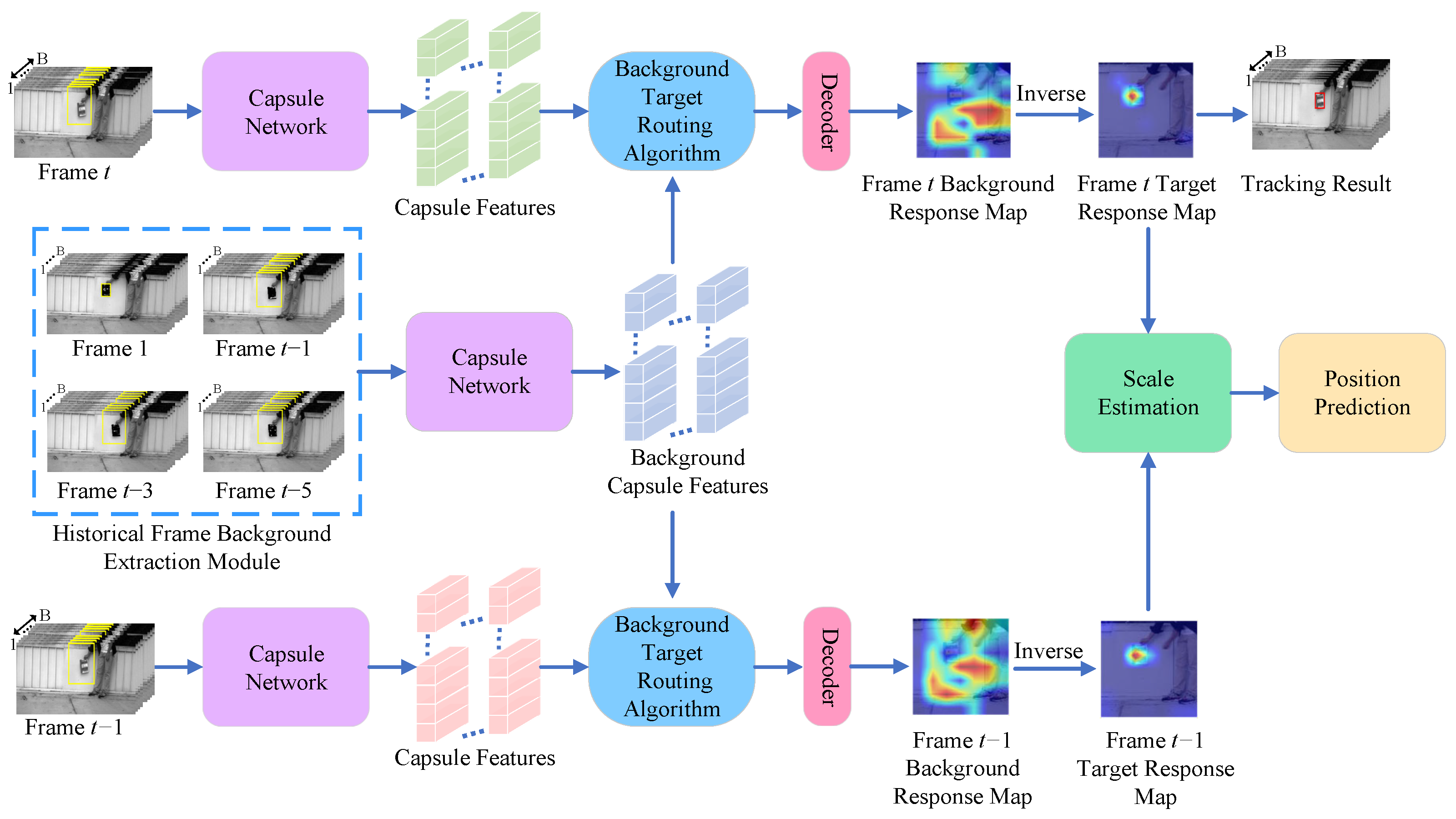
A NIR hyperspectral object tracking algorithm relying on background cues and spectral location estimation is proposed to tackle the issue of pixel-level data disparity between the target and background when the target varies. The method mainly uses background cues as the main information and target cues as the supplementary information for tracking. As illustrated in Figure 1, the proposed framework comprises three primary components: HFBE, BT, and SIP. In the HFBE module, the spectral information of the groundtruth of the first frame is used to spectral match frame t−1, frame t−3, and frame t−5 of input images to generate a mask thereby making a rough distinction between the target and the background. In the BT section, background features in the extracted HFBE module are used to match with the tth frame image search region features using the background similarity routing algorithm to generate a background capsule similar to the background. Finally, the network generates a background response map, which is subsequently converted into a target response map used to determine the location of the target. In the SIP module, predicted positions from the previous and current frames are used to determine the search region in the next frame, ensuring stable tracking of the target.
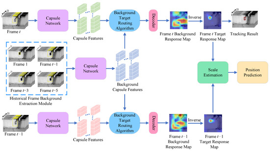
Figure 1.
The general structure of the designed algorithm.
3.1. Historical Frame Background Extraction Module
By extracting background information, the tracking algorithm can distinguish between the target and the background more effectively. This helps to reduce the occurrence of false detections and false tracking, especially in scenes with complex backgrounds or high interference in NIR hyperspectral target tracking. And the background information can provide additional contextual information, so that the tracking algorithm can still maintain stable tracking of the target through changes in the background when the target is partially occluded or deformed.
In order to obtain rich background information, we build a Historical Frame Background Extraction Module. It is taken into account that images neighboring the current frame in the time dimension contain more information similar to the current frame because they are closer in time. This means that the position and appearance of the target in adjacent frames may be similar because the target usually does not change much over a short period of time. Images farther from the current frame contain more original information because the time interval between them is longer. This means that in farther frames, the location, appearance, etc., of the target change significantly. Therefore, these images contain more raw information that has not been filtered or processed. Therefore, the selected background pool consists of the first four frames relative to the current one, i.e., frames 1, , , and . In HFBE, the missing video frames are interpolated. First, normalize the HSI of the target area in frame 1 and the search area in frame t (centered on the centroid of the target):
where represents the normalization of the HSI of the target area , denotes the i-th band of the t-th frame in , denotes the j-th pixel of , is the height of , and is the width of .
We use a global spectral curve to represent the spectral information at frame t. The global spectral curve is determined using the following procedure:
where represents the global spectral curve, and indicates its value at the i-th spectral band, with B denoting the total number of bands. The spectral curve represents the spectral response values of a specific point or region across multiple spectral bands, where the horizontal axis denotes the band index, and the vertical axis indicates the normalized pixel value. represents the normalized pixel value of , where t is a variable indicating the frame index in the hyperspectral video sequence.
In the target area of the first frame , a small portion of the background is involved in the target area because the target is irregular. In order to accurately find the pixels that best represent the target in a target region containing background pixels, it is necessary to classify the target region based on pixel grayscale values using statistical methods. We consider this method as a statistical approach because it utilizes the statistical properties of the pixel grayscale values in the image for classification. Specifically, we define a quantization process, where the grayscale value of each pixel is mapped to discrete levels, with a parameter controlling the number of levels. In this way, we are able to distinguish between target pixels and background pixels based on the grayscale distribution. This is specifically achieved as follows:
where is the label of each pixel, which is an integer ranging from 0 to 9, is the downward rounding operation, and is the remainder operation. represents the total number of gray scale range classifications. When the value of is larger, the accuracy of pixel segmentation in the target area of the first frame increases, and the computational complexity also rises. Conversely, a smaller value of results in reduced segmentation precision within the target region of the initial frame, along with lower computational overhead. Experimental results indicate that setting to 10 yields the most favorable performance. In the experiments, we tested different values of at intervals of 5, , and observed their impact on segmentation accuracy. When , some background pixels were misclassified as target pixels, leading to poor segmentation results and low distinction between the target and background. On the other hand, when , although the distinction between the target and background improved, the computational complexity increased significantly due to the need to process more grayscale categories. Considering these factors, we concluded that is the optimal choice. It allows for the best possible distinction between the target and background while maintaining low computational complexity.
According to the grayscale range label and grayscale range index, the spectral pixel intensity and spectral number intensity of each pixel in each band image in the target area of the first frame are determined. This is specifically achieved as follows:
where l is the grayscale range index, is the spectral pixel intensity, and is the spectral number intensity.
For each bin of , and can be accumulated separately as:
The maximum gray index number for each band is computed using the following formulation:
where represents the index of the target pixel set on the i-th band, given that target pixels occupy the highest proportion within the region of interest. Therefore, the local target spectral curve can be calculated as:
where denotes the local target spectral curve, and indicates the value corresponding to the i-th spectral band, refers to the total intensity of target pixels on band i within the region of interest at frame 1, and represents the total target pixel number of band i in the target area in the first frame.
The region of the t frame search region that is similar to the target region of frame 1 is determined by computing the spectral angular distance between the local target spectral curve and the search region of the t-th frame. This is specifically achieved as follows:
where D is the value of the spectral angular distance, while denotes matrix transposition.
To separate the target and the background, a mask is generated by spectral angular distance. This is specifically achieved as follows:
where Y represents the generated mask, and Thr represents the set spectral angular distance threshold. Pixels with high similarity are labeled as 0, while those with low similarity are labeled as 1. The mask is sent to the background pool for training.
The generated mask Y is computed with the search region of frame t to produce final results. This is specifically achieved as follows:
where P is the images of the search area after mask processing.
The results of the proposed history frame background extraction module are shown in Figure 2. Figure 2a shows the local spectral profile of the target region at frame 1. Figure 2b shows background masks generated after the spectral angular distance between the search region and the local spectral curve in frame t. The original image after background extraction is shown in Figure 2c.
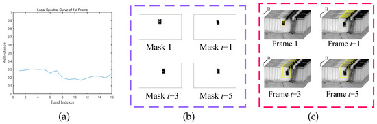
Figure 2.
Results of History Frame Background Extraction Module. (a) Spectral Curve of . (b) Generated Background Masks. (c) Final Results of Background Extraction.
3.2. Background Target Routing Algorithm
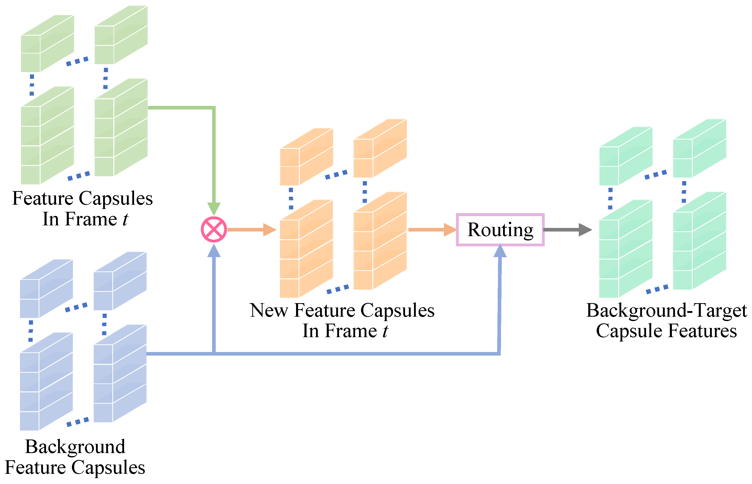
In HFBE, although the extracted background pixels typically constitute the majority of the pixels, there are still a few pixels that are mixed with the target information due to external factors such as noise. We employ a background similarity routing algorithm to ensure the purity of the background pixels. The algorithm is based on the principle of inter-capsule similarity [40]: when the i-th layer feature capsules show a high level of similarity with the j-th layer feature capsules, their weights increase accordingly. In order to achieve the complete elimination of target information from the background, we deliberately decrease the weight of target information to ensure that the final output is ideal background information. Figure 3 shows the process of the background target routing algorithm.
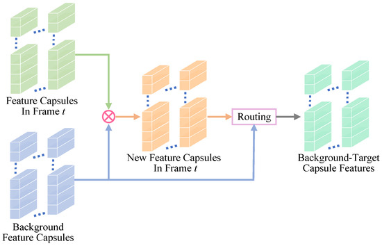
Figure 3.
The architecture of background similarity routing algorithm.
First, it computes the similarity between the feature capsule in frame t and the background feature capsule in the background pool. The new feature capsule in frame t that is similar to the background feature capsule is updated and obtained. In the next step, a routing algorithm is used to transfer information between the new feature capsule and the background feature capsule of the t frame. Thus, the background-target capsule feature (pure background capsule feature) of the current frame is generated. The feature capsule is updated using the similarity between the feature capsule and the background capsule of the feature capsule of the t frame. Then, the new feature capsule of frame t is routed with the background capsule to derive the background-only feature capsule of the current frame.
In order to calculate the similarity between the feature capsule and the background capsule at frame t. This is specifically achieved as follows:
where is the i-th background capsule, is the i-th feature capsule, and represents the magnitude of the vector. denotes the similarity between the background capsule and the feature capsule , which ranges from −1 to 1. In addition, 1 denotes that the two capsules are in the exact same direction, −1 denotes that the directions are completely opposite, and 0 denotes that the two capsules are orthogonal.
The generated new capsule is updated using the background capsule and the resemblance between the feature capsule so that the presence of the object capsule in the feature capsule of the tth frame is reduced. The new capsule is generated as follows:
where is the i-th feature capsule and denotes the difference in similarity from the background capsule to the signature capsule .
The weight coefficient between the background and the features is:
where is the weight coefficient between the i-th background capsule and the i-th feature capsule .
where denotes the output vector of the i-th capsule of the feature capsule in frame t after similarity processing.
The initial weight is initially set to 0. During iteration, the original weights are refreshed depending on the resemblance between each forecast capsule and the squashed weighted average capsule . The update of the initial weight can be expressed as:
where denotes the capsule obtained after compression with the squash function, as the next capsule j output. The larger is, the more consistent they are and the higher the preliminary weight will be. The smaller is, the weaker their similarity is and the preliminary weight decreases.
In the iterative process, the similar directions of all predicted vectors are found, and coupling coefficients are learned to be obtained. Normalization is performed with softmax so that the sum of coupling coefficients from the feature capsule i to all capsules in the background at frame t is one. The coupling coefficient is normalized weight, which is calculated as follows:
where is the coupling coefficient, k is the number of initial weights, represents the exponential function, and ∑ stands for the summing operation. At the beginning, routing weights from each feature capsule to all background capsules may be equal.
The total input to the next layer of capsule j is a weighted average of the output vectors predicted for that capsule by all capsules in the previous layer. This is specifically achieved as follows:
where denotes the total input of capsule j.
The total input of capsule is squashed so that the length is in the range of 0 to 1 to get the output. The squashing function acts similarly to the activation function of a convolutional neural network. It is expressed as:
where is the output of capsule j and is the total input of capsule j. When tends to 0, tends to 0. When tends to , tends to 1. The squash function is able to compress the length and keep the direction of the vector unchanged.
The decoders in Figure 1 belong to the decoder structure within the capsule network framework [40]. The background target capsule features generated are used to resize the output feature capsule through a decoder. Subsequently, these features are amplified by three transposed convolutional layers. Then, a standard convolutional layer is added with a convolutional kernel size of , a step size of 1, zero padding, and the number of output channels is 1. Finally, a single-channel background response map with the size of the search area is obtained. In Figure 1, the red portion of the Background Response Map indicates a highly responsive region as the background region, and the blue portion is a low responsive region as the target region. The parameters of the background response map were adjusted according to the literature [41] to derive the target response map.
Loss functions include capsule loss and regression loss. The capsule loss is:
where is the current capsule presence value of 0.9, is the current capsule absence value of 0.1, represents damage decrease weights for absent capsules, which are used to reduce the length of the numeric capsule vector with a value of 0.5. has a value of 1 when the k-th capsule is present and 0 otherwise.
The regression loss is calculated using the GIOU loss [54]:
where A is the forecast box, B is the hand-labeled ground truth box, and C is the smallest border rule between the forecast box and the goal box. Thus, the total loss is the combination of the capsule loss and the regression loss. This is specifically achieved as follows:
where is used to balance the regression loss weights for capsule loss and regression loss.
3.3. Spectral Information Position Prediction
A capsule network has higher computational complexity when dealing with HSI because it processes each feature into vectors for output. Searching within the predicted search box in the next frame can reduce computational complexity and locate the target area more accurately than searching the entire image range. It enhances tracking performance in terms of both responsiveness and precision. When the target is moving fast or the shape changes suddenly, the traditional strategy of fixing center of the search frame may lead to loss of the target. Predicting the position of the search frame in the next frame can better cope with these challenges and maintain stable tracking.
Using the capsule network to predict the frame at time t and the adjacent frame at time t−1, where the target is located at and , respectively.
where denotes the position of the target center at t-th frame, indicates the horizontal coordinate of the target at frame t, and represents the vertical coordinate.
where indicates the center position of target at the -th frame, refers to its horizontal coordinate, and corresponds to the vertical one.
In the case where relying only on the target center position to estimate the search center position in the subsequent frame may lead to a large error, we therefore approach the representation of the target by adding spectral information. When selecting the region where the target is located, we face a tradeoff problem: if the selected region is too large, it may contain too much background information, which introduces unnecessary errors; if the selected region is too small, it may not be possible to adequately capture important information about the target, which can also influence tracking accuracy. There is a need to use the box in the network output where the target is situated as the size of the selection region to solve this problem. The advantage of this approach is that the target box in the network output is usually learned based on extensive training data and can more correctly represent the location and size of the object in the current frame. Therefore, using this box as the selection region can ensure, to a certain extent, that it will not introduce too much background information and can fully contain the important features of the target.
Firstly, the average spectral information of the current frame and the adjacent frame is obtained respectively as:
where denotes the spectral curve on the B bands in frame t, represents the spectral curve of the i-th band at frame t, i denotes the i-th band, and j denotes the j-th pixel. The number of B in the dataset used in this paper is 16. denotes the target box of frame t, and denotes the averaging operation:
where denotes the target box of frame t, The height and width of are represented by and , respectively. represents the j-th pixel of the i-th band in the target region at frame t.
where denotes the spectral curve on the B bands in frame t, represents the grayscale value of the i-th band at frame t, i and j refer to the indices of the i-th spectral band and the j-th pixel, respectively. The number of B used in this paper is 16. denotes the target box of frame t and denotes the averaging operation:
where denotes the target box of frame , represents the number of rows in , represents the number of columns in , represents the total number of pixels in , and represents the j-th pixel of the i-th band in the target region at frame .
The position difference is obtained by calculating the position and , corresponding to the current and previous frames, respectively. This is specifically achieved as follows:
where denotes the position difference, with and indicating the target center locations at frames t and , respectively.
The spectral curve difference f is calculated from and as:
where f denotes the spectral curve differernce. If this value of f is closer to 0, we can assume that and are more similar on the band interval. In practice, due to the precision limitations of numerical calculations, we cannot directly obtain the case where the value of f is exactly equal to 0. Therefore, if the value of f is less than some very small positive number, we consider the two functions to be similar.
The spectral curve difference f determines whether the objects in the frames t and exhibit similarity. This is specifically achieved as follows:
where represents whether two objects are similar, and is the spectral positive number. Below the spectral positive number, it is similar and judged to be the same object, and the next position prediction is performed. If it is not an object, the information from the previous frame is updated into the Section 3.1 for subsequent tracking. Position prediction is performed as follows:
where represents the centre of the search area. The location of the next frame is used as the centre point of the search area to select the search area for tracking the next frame.
3.4. Experimental Setup
The proposed training and inference phases of the algorithm are actualized on NVIDIA RTX 3090 GPUs (NVIDIA, Santa Clara, CA, USA) using PyTorch 2.1.0 in Python 3.9. Our model is implemented based on the original CapsNet architecture proposed by Sabour et al. [40], which utilizes dynamic routing between capsules to encode spatial and part-whole relationships. On this basis, we modify the routing algorithm of the CapsNet and update the capsule weights using spectral information. Furthermore, we design modules such as HFBE, BT, and SIP to enhance spectral-spatial representation and improve adaptability in challenging tracking scenarios. The experimental training data parameters are as follows: in HFBE is set to 0.28 for distinguishing the target from the background, and the spectral positive number in SIP is set to , in the capsule loss function is set to 0.5, and in the total loss function is set to 0.5. The Adam optimization algorithm is used during training. We trained the network with a training rate of 0.0001 for offline practice. The learning rate was set to 0.0003 for the online refresh. The iterative routing experiments were set to 3 times.
The dataset HOT2023 [49] is used in this study. The HOT2023 dataset is accessible at www.hsitracking.com (accessed on 7 April 2025). The dataset was acquired at 25 FPS using three XIMEA fast cameras (including VIS, NIR, and RedNIR). They cover 16 bands, 25 bands, and 15 bands respectively. These include 182 training videos and 89 validation videos. HOT2023 contains NIR data at 665–960 nm, RedNIR data at 600–850 nm and hyperspectral data (VIS) at 460–600 nm. The video scenes involve 19 challenging conditions.
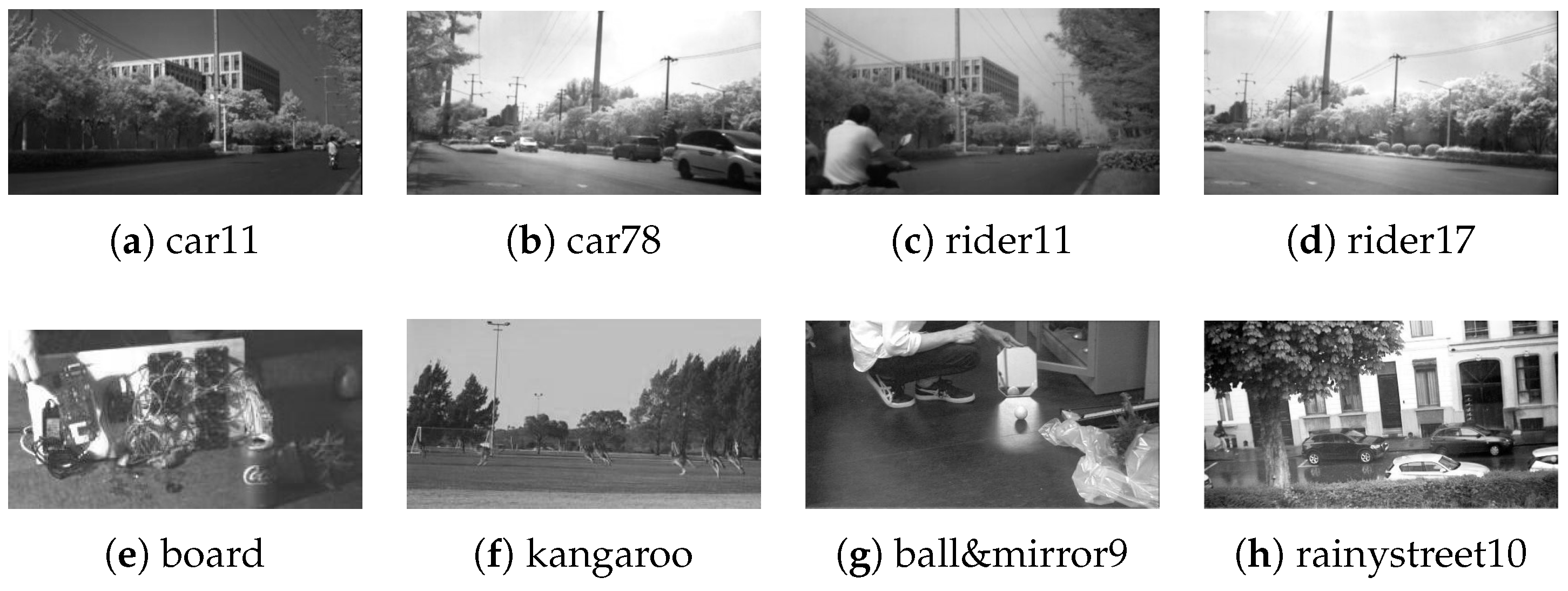
As shown in Figure 4, we selected four NIR data sequences (car11, car78, rider11, and rider17) and four hyperspectral data sequences (board, kangaroo, ball&mirror9, and rainystreet10) in the HOT2023 dataset.

Figure 4.
Eight sequences in the HOT2023.
Table 1 displays more details about the variables of the eight test sequences, and Figure 4 shows the false-color images of the eight sequences. We selected specific sequences from the eight test sequences. In particular, we selected sequences with different challenges such as background clutter (BC), scale variation (SV), fast motion (FM), in-plane rotation (IPR), motion blur (MB), occlusion (OCC), and out-of-plane rotation (OPR) in order to fully evaluate the generalization ability of the tracker.

Table 1.
Frames, Resolution, Initial Size, Challenges of the test sequences.
In our experimental design, the images processed by the selected RGB tracker are not directly derived from any three bands of the original hyperspectral data. Instead, the pseudo-color image sequence optimized by the HOT2023 dataset is used. The generation of pseudo-color images ensures the best contrast, rich texture information, and distinct target recognition features for the target tracking task. These pseudo-color images can effectively capture the characteristics of the original NIR and VIS data, maintaining a high degree of consistency with the original inputs in the target tracking task.
3.5. Evaluation Metrics
The success rate [55] reflects the estimation accuracy of the predicted bounding box, which is the percentage of all frames in which the overlap area of the target and the ground truth bounding boxes is above a threshold. The overlap score is calculated as
where is the target bounding box area of our algorithm, and is the area of the ground truth. As discussed, when the overlap between the bounding boxes exceeds a threshold, the tracking is considered successful. Specifically, for the coordinate system of the success rate curve, the x-axis denotes a series of continuous thresholds from 0 to 1, with different thresholds set. Similarly, the y-axis is the success rate. The precision rate [56] reflects positioning precision, which is the percentage of all frames in which the distance between the center of the predicted target bounding box and the ground truth is less than a threshold. The distance F between the center point of the target bounding box center and the ground truth value is calculated as
where is the center point of the ground truth, and is the predicted center point of the target bounding box. Specifically, for the coordinate system of the precision rate curve, the x-axis is a series of continuous thresholds from 0 to 50, and the y-axis is precision. The average distance precision rate is reported at a threshold of 20 pixels (DP@20). Additionally, we used the area under the curve (AUC) to measure the performance of each tracking algorithm.
4. Results and Analysis
4.1. Comparative Experiments
We compared the performance of the proposed algorithm with six state-of-the-art (SOTA) hyperspectral tracking algorithms in this experiment, i.e., MHT [49], SiamBAN [15], SiamCAR [45], SiamGAT [46], STARK [47], and TransT [1]. MHT uses different materials with different spectral information to differentiate between similarly colored objects, and SiamBAN uses a full convolutional network approach to classify the target and background and regress to the target frame. The SiamCAR approach is similar to SiamBAN in that it proposes centrality branches to update the predicted centroids. In contrast to SiamGAT, which introduces a target-aware selection mechanism, SiamCAR exhibits limited adaptability in handling target deformations. STARK uses intermediate frame information as a dynamic template and updates the template based on the transformer architecture. As for TransT, this network effectively fuses templates and searches for region features using only attention. It is worth noting that our proposed method is based on capsule networks and is not directly inspired by any of the compared methods. By comparing the proposed tracker algorithm with these SOTA algorithms, it is our goal to prove its usefulness and contendability in hyperspectral tracking applications.
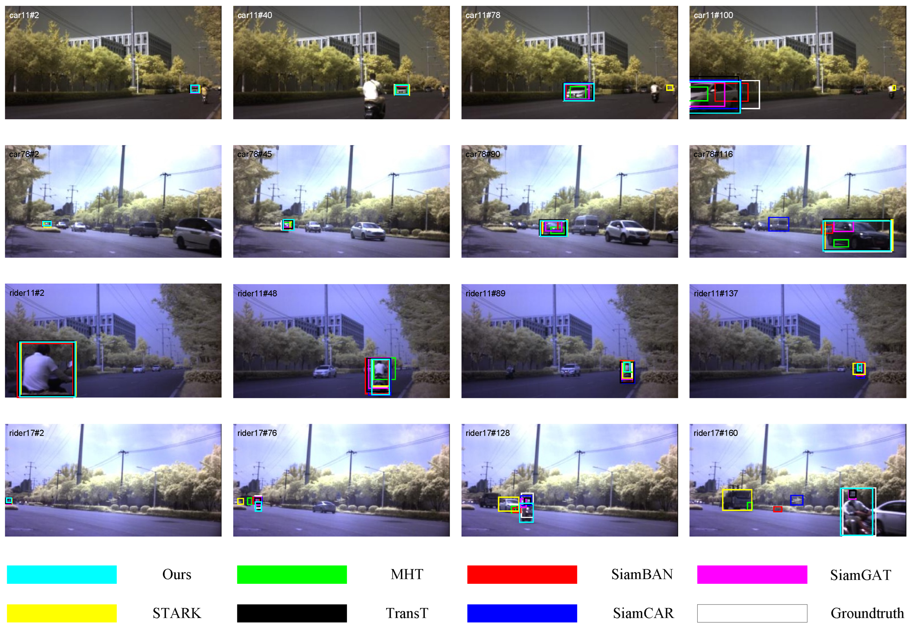
Figure 5 provides a visual summary of the tracking performance of our proposed method, benchmarked against six SOTA approaches across four distinct video sequences from the NIR dataset. In the figure, the various algorithms are clearly distinguished by rectangular boxes of different colors, where sky blue marks our proposed algorithm, green represents the classical MHT algorithm, red denotes the SiamBAN algorithm, pink-purple is the SiamGAT algorithm, blue is the SiamCAR algorithm, yellow highlights the STARK algorithm, black represents the TransT algorithm, and white represents the Groundtruth. Given the numerous rectangular boxes in the figure, it seems challenging to visually assess the strengths and weaknesses of each algorithm directly. We further utilized precision and success plots to quantitatively and intuitively evaluate the tracking performance of each method. These two graphs not only accurately reflect the precision and stability of the algorithms in the tracking process, but also facilitate us to quickly identify which algorithms have the best performance on specific sequences. Through this comprehensive analysis, we can evaluate the advantages and disadvantages of each algorithm in a more scientific way, and offer solid support for the subsequent optimization and deployment of the algorithms.

Figure 5.
Qualitative results on NIR four sequences.
The first row of Figure 5 shows the tracking results for the car11 sequence. A white car is traveling fast on the road. The pedestrian driving a battery-operated car completely obscures the white car at frame 49, which is a great challenge for trackers that rely on material information features for tracking. In the experiment, when running to the 78th frame, the traveling car undergoes scale deformation due to the limitation of the camera angle, and appears to be nearer and farther away. When the target is occluded, the keypoints on which the STARK algorithm relies may be lost or become invisible, leading to target loss. At the 100th frame, the car is moving fast, causing the MHT algorithm, SiamBAN algorithm, and SiamGAT algorithm to possibly not accommodate changes in target position and scale adjustments in a timely manner in terms of update frequency and scale adjustments, resulting in degradation of tracking accuracy.
The second row of Figure 5 shows the tracking result of the car78 sequence. The black car traveling from near to far is obscured by the tree and flower beds on the side of the road at frame 22. It is only after 45 frames that the full target silhouette appears. This also resulted in tracking drift. At around frame 90, the fast-moving car makes the hypothesis management and validation process of the MHT algorithm and the SiamGAT algorithm unable to stay abreast of rapid changes in goals, affecting tracking accuracy. At around frame 116, the car undergoes a large shape change, causing the SiamCAR algorithm to lose the target in subsequent frames.
The third row of Figure 5 shows the tracking results for the rider11 sequence. The rider is traveling on the road from near to far in the frame. In the experiment, around the 48th frame, the SiamCAR algorithm and the SiamBAN algorithm, which lack the long-time history information to predict the fast-moving trajectory of the target well, affect the stability of the tracking.
The last row of Figure 5 shows the tracking result of the rider17 sequence. A pedestrian riding an electric bike slowly appears in the frame from far and near. It is also shown as a small square target around frame 40 due to occlusion, and after frame 65, it is shown as a vertical rectangular target. In the experiments, when running up to about 128 frames, the low resolution image leads to difficulty in extracting the edge and detail-blurring features of the target. This can cause the algorithm to have trouble discriminating the target from the background and impacts the ability to match features accurately. It greatly affects the STARK algorithm, SiamGAT algorithm, and SiamBAN algorithm. Low-resolution images often struggle to capture changes in the overall appearance of the target, making it difficult for the tracking algorithms to accurately estimate the scale size of the target. This also leads to the fact that around frame 160, only our algorithm is able to accurately frame the entire pedestrians and vehicles with little difference from the true values.
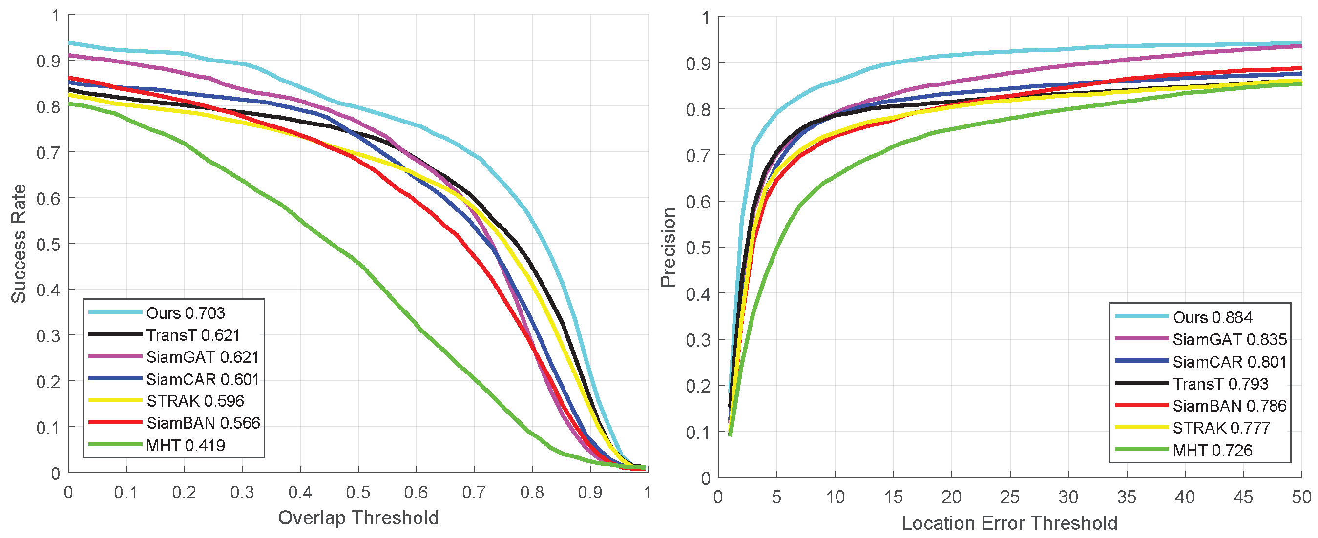
In the success and precision curve charts presented in Figure 6, a comprehensive performance evaluation of seven different tracking algorithms is performed for the NIR subset of the HOT2023 dataset. This analysis not only includes the precision of the algorithms in predicting the bounding box (success rate) but also carefully explores their positioning precision. As clearly seen in the figure, our proposed tracking algorithm demonstrates excellent performance on the overall video sequence. The success rate is as high as 70.3% while maintaining an accuracy level of 88.4%. Both of these metrics are significantly ahead of the other six compared algorithms and are firmly at the top of the list.
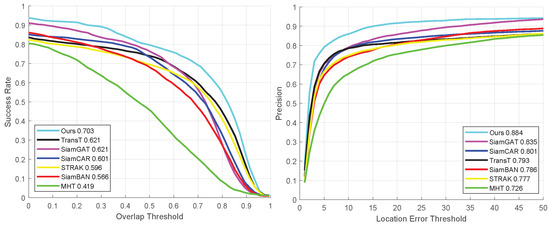
Figure 6.
Quantitative experimental results of all sequences in the NIR dataset.
As shown in Table 2, to highlight the effectiveness and uniqueness of our proposed algorithm, we further evaluate its performance across various challenging scenarios in the NIR hyperspectral tracking dataset, including FM, LR, OCC, and SV challenges. Unlike existing trackers such as SiamCAR, STARK, and SiamGAT that rely solely on spatial or temporal features, our algorithm fully exploits the spectral dimension and background information through a series of carefully designed modules. Specifically, in the FM challenge, where the target undergoes large displacements, our algorithm achieves the highest success rate of 76.8%. This is largely due to SIP, which predicts the likely target location by leveraging the spectral and positional continuity across frames. In contrast, SiamCAR depends on centrality-based branching, which struggles under large target movements, resulting in a 10.7% lower success rate. When facing the LR challenge, our algorithm outperforms STARK by 12.4%, benefiting from the use of spectral cues rather than just spatial-temporal dependencies. This advantage stems from HFBE, which constructs background templates from previous frames to improve target-background discrimination. Under occlusion scenarios, SiamGAT fails to utilize the spectral signature of the target effectively. In contrast, our algorithm integrates the BT module, which routes background capsules away from the target representation, allowing the model to maintain target localization even when partially obscured. This leads to a 9.1% improvement in success rate over SiamGAT. For the SV challenge, where spectral variability is high, our tracker maintains a strong 74% success rate by continuously adapting to the spectral characteristics of the target. While MHT exploits material properties to improve robustness, its inability to estimate target scale limits its accuracy, highlighting the superior adaptability and tracking precision of our model.
Table 2.
The AUC comparison on NIR/false-color videos. The highest and second-highest values are marked in red italics and blue bold, respectively.
Figure 7 intuitively summarizes the tracking performance of the proposed algorithm on the VIS dataset, using four representative video sequences, in comparison with six other SOTA algorithms.
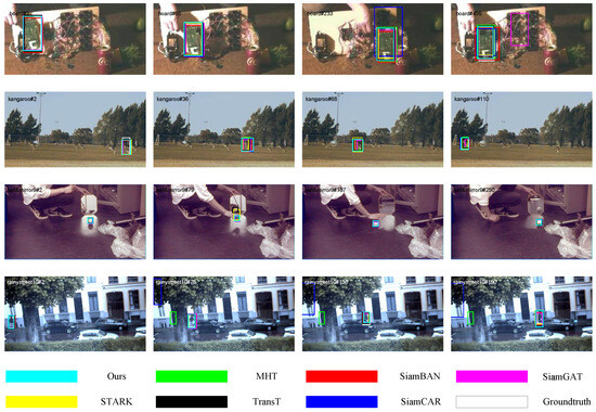
Figure 7.
Qualitative results on VIS four sequences.
The first row of Figure 7 shows the tracking results of the board sequence. As the hand moves, the board appears to rotate planarly, and after 167 frames, a coke bottle on the floor obscures a portion of the board. Around frame 456 in the experiment, cluttered objects in the background (e.g., wires and other electronic components) interfered with the feature extraction and detection of the tracker, causing the SiamGAT algorithm to mistake parts of the background for the target.
The second row of Figure 7 shows the kangaroo sequence tracking outcomes. The quick hopping of kangaroos and the resemblance between stalked kangaroos and their fellow kangaroos caused some motion blur and background interference. However, the majority of the trackers show good performance in this sequence as they rely heavily on the target features. Thus, despite the presence of background interference and multiple similar targets, the trackers are able to maintain tracking stability and accuracy for the target kangaroo by recognizing and matching these features.
The third row of Figure 7 shows the tracking results for the ball&mirror9 sequence. The target white ball becomes blurred due to reflections in the mirror. In the experiment, at around frame 79, artefacts or unrealistic highlight areas appear in the mirror, which may visually have similar characteristics to the actual target, causing the TransT algorithm to incorrectly track the reflected ball in the mirror.
The last row of Figure 7 shows the tracking results for the rainystreet10 sequence. At around frames 48 and 102, the tree and the car in the frame completely occlude or partially occlude the pedestrians, respectively, and under prolonged or severe occlusion, the tracker may lose track of the target completely. In the experiment, at frame 78, the MHT method and the SiamCAR method lost the target due to the prolonged occlusion of the tree before and failed to retrieve the target in the subsequent frames.
In the results of the quantitative experiment presented in Figure 8, a comprehensive performance evaluation of seven different tracking algorithms is performed for a subset of the VIS in the HOT2023 dataset. This analysis not only covers the success rate of the algorithms in the prediction of the bounding box, but also takes a close look at their precision of localization. It is clearly visible from the figure that our proposed tracking algorithms demonstrate excellent performance on the overall video sequences. The success rate is as high as 59.6% while maintaining an accuracy level of 78.8%. These two metrics are significantly ahead of the other six compared algorithms.
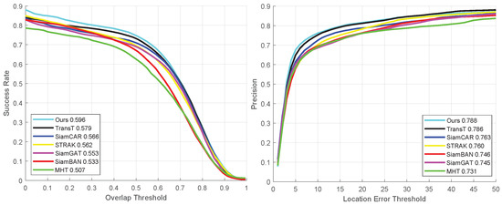
Figure 8.
Quantitative experimental results of all sequences in the VIS dataset.
To better quantify and visualize the advantages of our algorithms, Table 3 details the specific scores of each algorithm under the 19 challenging scenarios faced by the VIS dataset. Our tracker demonstrates superior tracking results against the complex challenges of BC, IPR, LR, OCC, OPR, and SV, fully proving its robustness and adaptability. It ranks second among trackers in DEF, FM, and LL challenges. Our algorithm demonstrated excellent performance in the BC challenge, achieving a success rate of 60.2%. In comparison, SiamCAR ranks second with a success rate of 59.2%, mainly in the interference processing of target information in the BC challenge. It is worth noting that our algorithm demonstrates its unique advantages in complex scenarios such as IPR, OCC, OPR, and SV. Unlike the TransT algorithm, which only relies on contextual information, we fuse the background information of historical frames with the spectral features of the target. This strategy allows us to achieve significant performance improvements of 1.8%, 0.7%, 2.1%, and 1.3%, respectively, when facing the above challenges. However, under the DEF and LL challenges, the TransT algorithm is able to capture detail changes more acutely due to its built-in attention mechanism. Our algorithm faced a certain degree of challenge in DEF and LL, with a slight decrease in success rate of 0.1% and 1.1%. When faced with the FM challenge, our algorithm was unable to accurately capture the background due to its large variations, and the success rate only reached second place. This suggests that we need to further optimize the algorithm to better adapt to complex and changing environmental conditions in future research.
Table 3.
The AUC comparison on hyperspectral/false-color videos. The highest and second-highest values are marked in red italics and blue bold, respectively.
To demonstrate the broad applicability of the proposed algorithm, we performed cross-dataset validation using the VOT-NIR dataset and evaluated it using the same metrics as the HOT2023 dataset. Table 4 shows the accuracy, success rate, and running speed (FPS) of all comparative algorithms on all video sequences in the VOT-NIR dataset.
Table 4.
The success rate and precision rate of all sequences in VOT-NIR. The highest and second-highest values are marked in red italics and blue bold, respectively.
As shown in Table 4, the proposed algorithm achieves the best success rate and accuracy, with a success rate of 0.699 and a precision of 0.872, which are 5.8% and 1.5% higher than the second-place method, respectively. Compared to the latest Siamese network-based tracker, SiamGAT, the proposed algorithm improves the success rate by 6.2% and the precision by 1.5%. SiamGAT enhances the Siamese framework by introducing a graph attention mechanism that establishes part-to-part correspondence between the target and search regions, effectively overcoming the limitations of traditional cross-correlation methods. However, it does not fully exploit spectral information. In contrast, our algorithm fully leverages the spectral dimension and background information through a series of carefully designed modules. Compared to the Transformer-based tracker TransT, the proposed algorithm improves the success rate by 5.8% and the precision by 4.9%. TransT replaces traditional correlation methods with attention-based modules, alleviating the issue of semantic information loss and overcoming the limitations of local matching. However, TransT performs poorly when handling OCC or SV. The SIP module we designed utilizes the position and spectral information of neighboring frames and the current frame to determine the search area for the next frame, effectively addressing the challenges of OCC and SV. Despite the inherent complexity of the proposed capsule network algorithm, which results in a higher computational load, its running speed reaches 42.6 FPS, meeting the real-time requirements of 25 FPS in typical video scenarios.
4.2. Ablation Experiments
To validate the performance of this proposed algorithm for each module, we conducted ablation experiments using the NIR dataset. The experimental results are shown in Table 5: (i) When all three modules of this algorithm are used, the tracking algorithm achieves a success rate of 70.3% and an accuracy of 88.4%, running at 40.5 FPS. (ii) Removing the SIP and not predicting the search region results in a decrease in success rate, with the tracking operating at 13.8 FPS; this demonstrates the efficacy of the Spectral Information Position Prediction in reducing computational complexity. Due to the fact that the entire capsule network of tracking is complete, few targets are lost, which also suggests that predicting the search area for the next frame is something that is practical for this algorithm. In addition, (iii) uses a normal capsule network to capture the correlation that exists among the object and backdrop without the use of BT, which shows that the importance of the spectral information is very significant, with a reduction of 19% compared to (i) and a tracking run speed of 50.2 FPS. The (iv) uses only the HFBE module and employing a detection-based capsule network framework for the remaining tracking tasks results in a success rate of 50.1% at 36.7 FPS. The (v) algorithm does not use HFBE and the success rate reaches 56.3% at 69.0 FPS, which is 4% lower than (i), indicating that BT is useful for this algorithm. (vi) Our algorithm uses only BT and achieves a success rate of 52.6% at 39.3 FPS, which compares favorably with the algorithm of (iv), in which the importance of using spectacular spectral information to distinguish between different capsule weights can be seen. (vii) demonstrates the case when SIP is used in a detection-based capsule network framework for prediction of the search area, the success rate is only 32.6% at 112.6 FPS. (viii). We replaced the BT routing algorithm with the lightweight architecture MobileNetV4. MobileNetV4 combines efficient design in deep learning models with Neural Architecture Search (NAS), achieving higher performance and computational efficiency. The experimental results show that replacing BT routing algorithm with MobileNetV4 led to a 20.5% decrease in success rate, a 27.4% decrease in Precision, and a 92.3 increase in fps. The decrease in success rate and precision can be attributed to the fact that MobileNetV4 primarily optimizes computational efficiency and memory usage, aiming to provide a lightweight network architecture, while capsule networks excel in modeling spatial relationships, particularly in handling dynamic and deformable objects. However, MobileNetV4 is more advantageous for real-time deployment.
Table 5.
Ablation study on NIR. ✓ indicates that the module is enabled, while ✗ indicates that the module is disabled.
5. Conclusions
This work presents a novel near-infrared hyperspectral video tracking methodology grounded in capsule-based architecture, integrating background modeling with spectral-spatial to achieve robust target localization. The method distinguishes between the target and background in the current frame using spatial and spectral information. Additionally, the background target routing algorithm effectively handles rapid target movement and scale changes. Finally, a spectral information position prediction module is introduced to reduce the sensitivity of the network to search region selection, thereby enhancing tracking accuracy. The effectiveness of the proposed algorithm is validated by experimental results, with an accuracy of 88.4% and a success rate of 70.3% in NIR tests. However, our proposed algorithm currently underperforms when faced with BC in the NIR dataset. In the future, we aim to further improve the algorithm to overcome this challenge. In addition, due to the inherent complexity of capsule networks, which may hinder their real-time deployment, we plan to combine lightweight network architectures with capsule networks in the future to maintain high accuracy while improving speed and real-time deployment efficiency.
Author Contributions
Conceptualization, L.W. and M.W.; substantial contributions to the conception, M.W.; interpretation of data for the work, M.W., K.H. and W.Z.; drafting the work or reviewing it critically for important intellectual content, M.W. and W.Z.; final approval of the version to be published, M.W., K.H., W.J. and W.Z.; investigation, M.W., K.H., W.J. and W.Z.; resources, M.W.; data curation, M.W., K.H. and W.Z.; writing—original draft preparation, M.W.; writing—review and editing, L.W., W.Z. and J.L.; visualization, M.W., K.H. and W.Z.; supervision, D.Z., L.W. and J.L.; project administration, D.Z., L.W. and J.L.; funding acquisition, D.Z. All authors have read and agreed to the published version of the manuscript.
Funding
This work was supported in part by the Wuxi Innovation and Entrepreneurship Fund “Taihu Light” Science and Technology (Fundamental Research) Project under Grant K20221046, and in part by the 111 Project under Grant B17035.
Data Availability Statement
The raw data supporting the conclusions of this article will be made available by the authors on request.
Acknowledgments
Thanks are due to Xuguang Zhu and Jialu Cao for the valuable discussions.
Conflicts of Interest
The authors declare no conflicts of interest.
References
- Chen, X.; Yan, B.; Zhu, J.; Wang, D.; Yang, X.; Lu, H. Transformer tracking. In Proceedings of the IEEE/CVF Conference on Computer Vision and Pattern Recognition (CVPR), Nashville, TN, USA, 20–25 June 2021; pp. 8126–8135. [Google Scholar]
- Chen, X.; Peng, H.; Wang, D.; Lu, H.; Hu, H. Seqtrack: Sequence to sequence learning for visual object tracking. In Proceedings of the IEEE/CVF Conference on Computer Vision and Pattern Recognition (CVPR), Vancouver, BC, Canada, 17–24 June 2023; pp. 14572–14581. [Google Scholar]
- Yu, Y.; Xiong, Y.; Huang, W.; Scott, M.R. Deformable siamese attention networks for visual object tracking. In Proceedings of the IEEE/CVF Conference on Computer Vision and Pattern Recognition (CVPR), Seattle, WA, USA, 13–19 June 2020; pp. 6728–6737. [Google Scholar]
- Feng, W.; Meng, F.; Yu, C.; You, A. Fusion of Multiple Attention Mechanisms and Background Feature Adaptive Update Strategies in Siamese Networks for Single-Object Tracking. Appl. Sci. 2024, 14, 8199. [Google Scholar] [CrossRef]
- Kristan, M.; Leonardis, A.; Matas, J.; Felsberg, M.; Pflugfelder, R.; Kämäräinen, J.K.; Danelljan, M.; Zajc, L.Č.; Lukežič, A.; Drbohlav, O.; et al. The eighth visual object tracking VOT2020 challenge results. In Proceedings of the European Conference on Computer Vision (ECCV), Glasgow, UK, 23–28 August 2020; pp. 547–601. [Google Scholar]
- Zheng, L.; Tang, M.; Chen, Y.; Zhu, G.; Wang, J.; Lu, H. Improving multiple object tracking with single object tracking. In Proceedings of the IEEE/CVF Conference on Computer Vision and Pattern Recognition (CVPR), Nashville, TN, USA, 20–25 June 2021; pp. 2453–2462. [Google Scholar]
- Voulodimos, A.; Doulamis, N.; Doulamis, A.; Protopapadakis, E. Deep learning for computer vision: A brief review. Comput. Intell. Neurosci. 2018, 2018, 7068349. [Google Scholar] [CrossRef]
- Bolme, D.S.; Beveridge, J.R.; Draper, B.A.; Lui, Y.M. Visual object tracking using adaptive correlation filters. In Proceedings of the IEEE/CVF Conference on Computer Vision and Pattern Recognition (CVPR), San Francisco, CA, USA, 13–18 June 2010; pp. 2544–2550. [Google Scholar]
- Kim, C.; Fuxin, L.; Alotaibi, M.; Rehg, J.M. Discriminative appearance modeling with multi-track pooling for real-time multi-object tracking. In Proceedings of the IEEE/CVF Conference on Computer Vision and Pattern Recognition(CVPR), Nashville, TN, USA, 20–25 June 2021; pp. 9553–9562. [Google Scholar]
- Olabintan, A.B.; Abdullahi, A.S.; Yusuf, B.O.; Ganiyu, S.A.; Saleh, T.A.; Basheer, C. Prospects of polymer Nanocomposite-Based electrochemical sensors as analytical devices for environmental Monitoring: A review. Microchem. J. 2024, 204, 111053. [Google Scholar] [CrossRef]
- Miranda, V.R.; Rezende, A.M.; Rocha, T.L.; Azpúrua, H.; Pimenta, L.C.; Freitas, G.M. Autonomous navigation system for a delivery drone. J. Control Autom. Electr. Syst. 2022, 33, 141–155. [Google Scholar] [CrossRef]
- Shamshad, F.; Khan, S.; Zamir, S.W.; Khan, M.H.; Hayat, M.; Khan, F.S.; Fu, H. Transformers in medical imaging: A survey. Med. Image Anal. 2023, 88, 102802. [Google Scholar] [CrossRef]
- Kiani Galoogahi, H.; Sim, T.; Lucey, S. Correlation filters with limited boundaries. In Proceedings of the IEEE/CVF Conference on Computer Vision and Pattern Recognition (CVPR), Boston, MA, USA, 7–12 June 2015; pp. 4630–4638. [Google Scholar]
- Fan, H.; Ling, H. Siamese cascaded region proposal networks for real-time visual tracking. In Proceedings of the IEEE/CVF Conference on Computer Vision and Pattern Recognition (CVPR), Long Beach, CA, USA, 15–20 June 2019; pp. 7952–7961. [Google Scholar]
- Chen, Z.; Zhong, B.; Li, G.; Zhang, S.; Ji, R. Siamese box adaptive network for visual tracking. In Proceedings of the IEEE/CVF Conference on Computer Vision and Pattern Recognition (CVPR), Seattle, WA, USA, 13–19 June 2020; pp. 6668–6677. [Google Scholar]
- Liu, H.; Zhao, Y.; Dong, P.; Guo, X.; Wang, Y. IOF-Tracker: A Two-Stage Multiple Targets Tracking Method Using Spatial-Temporal Fusion Algorithm. Appl. Sci. 2025, 15, 107. [Google Scholar] [CrossRef]
- Uzkent, B.; Rangnekar, A.; Hoffman, M. Aerial vehicle tracking by adaptive fusion of hyperspectral likelihood maps. In Proceedings of the IEEE/CVF Conference on Computer Vision and Pattern Recognition (CVPR), Honolulu, HI, USA, 21–26 July 2017; pp. 39–48. [Google Scholar]
- Jiang, X.; Wang, X.; Sun, C.; Zhu, Z.; Zhong, Y. A channel adaptive dual Siamese network for hyperspectral object tracking. IEEE Trans. Geosci. Remote Sens. 2024, 62, 5403912. [Google Scholar] [CrossRef]
- Wan, X.; Chen, F.; Liu, W.; He, Y. Artificial gorilla troops optimizer enfolded broad learning system for spatial-spectral hyperspectral image classification. Infrared Phys. Technol. 2024, 138, 105220. [Google Scholar] [CrossRef]
- Hameed, A.A.; Jamil, A.; Seyyedabbasi, A. An optimized feature selection approach using sand Cat Swarm optimization for hyperspectral image classification. Infrared Phys. Technol. 2024, 141, 105449. [Google Scholar] [CrossRef]
- Liu, C.; Chen, H.; Deng, L.; Guo, C.; Lu, X.; Yu, H.; Zhu, L.; Dong, M. Modality specific infrared and visible image fusion based on multi-scale rich feature representation under low-light environment. Infrared Phys. Technol. 2024, 140, 105351. [Google Scholar] [CrossRef]
- Xiong, J.; Liu, G.; Tang, H.; Gu, X.; Bavirisetti, D.P. SeGFusion: A semantic saliency guided infrared and visible image fusion method. Infrared Phys. Technol. 2024, 140, 105344. [Google Scholar] [CrossRef]
- Xiong, C.; Hu, M.; Lu, H.; Zhao, F. Distributed Multi-Sensor Fusion for Multi-Group/Extended Target Tracking with Different Limited Fields of View. Appl. Sci. 2024, 14, 9627. [Google Scholar] [CrossRef]
- Jia, L.; Yang, F.; Chen, Y.; Peng, L.; Leng, H.; Zu, W.; Zang, Y.; Gao, L.; Zhao, M. Prediction of wetland soil carbon storage based on near infrared hyperspectral imaging and deep learning. Infrared Phys. Technol. 2024, 139, 105287. [Google Scholar] [CrossRef]
- An, R.; Liu, G.; Qian, Y.; Xing, M.; Tang, H. MRASFusion: A multi-scale residual attention infrared and visible image fusion network based on semantic segmentation guidance. Infrared Phys. Technol. 2024, 139, 105343. [Google Scholar] [CrossRef]
- Shao, Y.; Kang, X.; Ma, M.; Chen, C.; Wang, D. Robust infrared small target detection with multi-feature fusion. Infrared Phys. Technol. 2024, 139, 104975. [Google Scholar] [CrossRef]
- Zhao, D.; Tang, L.; Arun, P.V.; Asano, Y.; Zhang, L.; Xiong, Y.; Tao, X.; Hu, J. City-scale distance estimation via near-infrared trispectral light extinction in bad weather. Infrared Phys. Technol. 2023, 128, 104507. [Google Scholar] [CrossRef]
- Amiri, I.; Houssien, F.M.A.M.; Rashed, A.N.Z.; Mohammed, A.E.N.A. Temperature effects on characteristics and performance of near-infrared wide bandwidth for different avalanche photodiodes structures. Results Phys. 2019, 14, 102399. [Google Scholar] [CrossRef]
- Renaud, D.; Assumpcao, D.R.; Joe, G.; Shams-Ansari, A.; Zhu, D.; Hu, Y.; Sinclair, N.; Loncar, M. Sub-1 Volt and high-bandwidth visible to near-infrared electro-optic modulators. Nat. Commun. 2023, 14, 1496. [Google Scholar] [CrossRef]
- Zhao, D.; Zhou, L.; Li, Y.; He, W.; Arun, P.V.; Zhu, X.; Hu, J. Visibility estimation via near-infrared bispectral real-time imaging in bad weather. Infrared Phys. Technol. 2024, 136, 105008. [Google Scholar] [CrossRef]
- Liu, Z.; Wang, X.; Zhong, Y.; Shu, M.; Sun, C. SiamHYPER: Learning a hyperspectral object tracker from an RGB-based tracker. IEEE Trans. Image Process. 2022, 31, 7116–7129. [Google Scholar] [CrossRef]
- Sarker, I.H. Deep learning: A comprehensive overview on techniques, taxonomy, applications and research directions. SN Comput. Sci. 2021, 2, 420. [Google Scholar] [CrossRef] [PubMed]
- Zhang, Z.; Hu, B.; Wang, M.; Arun, P.V.; Zhao, D.; Zhu, X.; Hu, J.; Li, H.; Zhou, H.; Qian, K. Hyperspectral Video Tracker Based on Spectral Deviation Reduction and a Double Siamese Network. Remote Sens. 2023, 15, 1579. [Google Scholar] [CrossRef]
- Li, Z.; Liu, F.; Yang, W.; Peng, S.; Zhou, J. A Survey of Convolutional Neural Networks: Analysis, Applications, and Prospects. IEEE Trans. Neural Netw. Learn. Syst. 2021, 33, 6999–7019. [Google Scholar] [CrossRef]
- Li, Z.; Xiong, F.; Zhou, J.; Lu, J.; Qian, Y. Learning a deep ensemble network with band importance for hyperspectral object tracking. IEEE Trans. Image Process. 2023, 32, 2901–2914. [Google Scholar] [CrossRef] [PubMed]
- Tang, Y.; Liu, Y.; Huang, H. Target-aware and spatial-spectral discriminant feature joint correlation filters for hyperspectral video object tracking. Comput. Vis. Image Underst. 2022, 223, 103535. [Google Scholar] [CrossRef]
- Wei, X.; Bai, Y.; Zheng, Y.; Shi, D.; Gong, Y. Autoregressive visual tracking. In Proceedings of the IEEE/CVF Conference on Computer Vision and Pattern Recognition (CVPR), Vancouver, BC, Canada, 17–24 June 2023; pp. 9697–9706. [Google Scholar]
- Zhu, Z.; Wu, W.; Zou, W.; Yan, J. End-to-end flow correlation tracking with spatial-temporal attention. In Proceedings of the IEEE/CVF Conference on Computer Vision and Pattern Recognition (CVPR), Salt Lake City, UT, USA, 18–23 June 2018; pp. 548–557. [Google Scholar]
- Li, W.; Hou, Z.; Zhou, J.; Tao, R. SiamBAG: Band attention grouping-based Siamese object tracking network for hyperspectral videos. IEEE Trans. Geosci. Remote Sens. 2023, 61, 5514712. [Google Scholar] [CrossRef]
- Sabour, S.; Frosst, N.; Hinton, G.E. Dynamic routing between capsules. In Advances in Neural Information Processing Systems; MIT Press: Cambridge, MA, USA, 2017; Volume 30, pp. 3859–3869. [Google Scholar]
- Ma, D.; Wu, X. Capsule-based regression tracking via background inpainting. IEEE Trans. Image Process. 2023, 32, 2867–2878. [Google Scholar] [CrossRef]
- Paoletti, M.E.; Haut, J.M.; Fernandez-Beltran, R.; Plaza, J.; Plaza, A.; Li, J.; Pla, F. Capsule networks for hyperspectral image classification. IEEE Trans. Geosci. Remote Sens. 2018, 57, 2145–2160. [Google Scholar] [CrossRef]
- Mei, Z.; Yin, Z.; Kong, X.; Wang, L.; Ren, H. Cascade residual capsule network for hyperspectral image classification. IEEE J. Sel. Top. Appl. Earth Obs. Remote Sens. 2022, 15, 3089–3106. [Google Scholar] [CrossRef]
- Ma, D.; Wu, X. Cascaded Tracking via Pyramid Dense Capsules. In Proceedings of the European Conference on Computer Vision (ECCV), Glasgow, UK, 23–28 August 2020; pp. 683–696. [Google Scholar]
- Guo, D.; Wang, J.; Cui, Y.; Wang, Z.; Chen, S. SiamCAR: Siamese fully convolutional classification and regression for visual tracking. In Proceedings of the IEEE/CVF Conference on Computer Vision and Pattern Recognition (CVPR), Seattle, WA, USA, 13–19 June 2020; pp. 6269–6277. [Google Scholar]
- Guo, D.; Shao, Y.; Cui, Y.; Wang, Z.; Zhang, L.; Shen, C. Graph attention tracking. In Proceedings of the IEEE/CVF Conference on Computer Vision and Pattern Recognition (CVPR), Nashville, TN, USA, 20–25 June 2021; pp. 9543–9552. [Google Scholar]
- Yan, B.; Peng, H.; Fu, J.; Wang, D.; Lu, H. Learning spatio-temporal transformer for visual tracking. In Proceedings of the Proceedings of the IEEE/CVF International Conference on Computer Vision, Montreal, QC, Canada, 10–17 October 2021; pp. 10448–10457. [Google Scholar]
- Wang, Y.; Huo, L.; Fan, Y.; Wang, G. A thermal infrared target tracking based on multi-feature fusion and adaptive model update. Infrared Phys. Technol. 2024, 139, 105345. [Google Scholar] [CrossRef]
- Xiong, F.; Zhou, J.; Qian, Y. Material based object tracking in hyperspectral videos. IEEE Trans. Image Process. 2020, 29, 3719–3733. [Google Scholar] [CrossRef] [PubMed]
- Zhu, Z.; Wang, Q.; Li, B.; Wu, W.; Yan, J.; Hu, W. Distractor-aware siamese networks for visual object tracking. In Proceedings of the European Conference on Computer Vision (ECCV), Munich, Germany, 8–14 September 2018; pp. 101–117. [Google Scholar]
- Bhat, G.; Danelljan, M.; Van Gool, L.; Timofte, R. Know your surroundings: Exploiting scene information for object tracking. In Proceedings of the European Conference on Computer Vision (ECCV), Glasgow, UK, 23–28 August 2020; pp. 205–221. [Google Scholar]
- Yang, Z.; Wei, Y.; Yang, Y. Collaborative video object segmentation by multi-scale foreground-background integration. IEEE Trans. Pattern Anal. Mach. Intell. 2021, 44, 4701–4712. [Google Scholar] [CrossRef] [PubMed]
- Yang, Z.; Wei, Y.; Yang, Y. Associating objects with transformers for video object segmentation. In Advances in Neural Information Processing Systems; MIT Press: Cambridge, MA, USA, 2021; Volume 34, pp. 2491–2502. [Google Scholar]
- Hu, J.; Shen, L.; Sun, G. Squeeze-and-excitation networks. In Proceedings of the IEEE/CVF Conference on Computer Vision and Pattern Recognition (CVPR), Salt Lake City, UT, USA, 18–23 June 2018; pp. 7132–7141. [Google Scholar]
- Chen, Y.; Yuan, Q.; Tang, Y.; Xiao, Y.; He, J.; Liu, Z. SENSE: Hyperspectral video object tracker via fusing material and motion cues. Inf. Fusion 2024, 109, 102395. [Google Scholar] [CrossRef]
- Chen, Y.; Yuan, Q.; Tang, Y.; Xiao, Y.; He, J.; Han, T.; Liu, Z.; Zhang, L. SSTtrack: A unified hyperspectral video tracking framework via modeling spectral-spatial-temporal conditions. Inf. Fusion 2025, 114, 102658. [Google Scholar] [CrossRef]


Disclaimer/Publisher’s Note: The statements, opinions and data contained in all publications are solely those of the individual author(s) and contributor(s) and not of MDPI and/or the editor(s). MDPI and/or the editor(s) disclaim responsibility for any injury to people or property resulting from any ideas, methods, instructions or products referred to in the content. |
© 2025 by the authors. Licensee MDPI, Basel, Switzerland. This article is an open access article distributed under the terms and conditions of the Creative Commons Attribution (CC BY) license (https://creativecommons.org/licenses/by/4.0/).