Article

Monocular Vision-Based Depth Estimation of Forward-Looking Scenes for Mobile Platforms

1
School of Information Engineering, Nanhang Jincheng College, Nanjing 211156, China
2
College of Civil Aviation, Nanjing University of Aeronautics and Astronautics, Nanjing 211106, China
*
Author to whom correspondence should be addressed.
Appl. Sci. 2025, 15(8), 4267; https://doi.org/10.3390/app15084267
Submission received: 27 February 2025 / Revised: 10 April 2025 / Accepted: 11 April 2025 / Published: 12 April 2025

Abstract

:
The depth estimation of forward-looking scenes is one of the fundamental tasks for an Intelligent Mobile Platform to perceive its surrounding environment. In response to this requirement, this paper proposes a self-supervised monocular depth estimation method that can be utilized across various mobile platforms, including unmanned aerial vehicles (UAVs) and autonomous ground vehicles (AGVs). Building on the foundational framework of Monodepth2, we introduce an intermediate module between the encoder and decoder of the depth estimation network to facilitate multiscale fusion of feature maps. Additionally, we integrate the channel attention mechanism ECANet into the depth estimation network to enhance the significance of important channels. Consequently, the proposed method addresses the issue of losing critical features, which can lead to diminished accuracy and robustness. The experiments presented in this paper are conducted on two datasets: KITTI, a publicly available dataset collected from real-world environments used to evaluate depth estimation performance for AGV platforms, and AirSim, a custom dataset generated using simulation software to assess depth estimation performance for UAV platforms. The experimental results demonstrate that the proposed method can overcome the adverse effects of varying working conditions and accurately perceive detailed depth information in specific regions, such as object edges and targets of different scales. Furthermore, the depth predicted by the proposed method is quantitatively compared with the ground truth depth, and a variety of evaluation metrics confirm that our method exhibits superior inference capability and robustness.

1. Introduction

An Intelligent Mobile Platform (IMP) is an advanced robotic system that operates autonomously without the need for direct human control. It is capable of autonomous sensing, decision-making, and task execution [1,2]. Unmanned aerial vehicles (UAVs) and autonomous ground vehicles (AGVs) are the primary examples of IMPs [3,4,5]. With the rapid advancement of artificial intelligence, IMPs have found extensive applications across various domains. Their high level of automation and strong adaptability to diverse environments provide them with a significant advantage over manned systems, especially in challenging working conditions. IMPs can effectively replace humans in hazardous tasks, thereby significantly reducing safety risks.
Environmental sensing is a fundamental task for ensuring the safe operation of IMPs [6]. Sensing technology equips IMPs with the capability to continuously detect potential obstacles, other traffic participants, terrain changes, and other factors that may jeopardize operational safety. This technology enables IMPs to take timely measures to avoid collisions or other hazardous situations [7,8]. A crucial component of environmental sensing is depth information, which refers to the distance of objects or points in the scene relative to the IMP’s sensor. Depth information is essential for IMPs to understand the spatial relationships between objects in the environment [9]. Therefore, the primary objective of this paper is to obtain depth information from the forward-looking scene during the operation of an IMP, thereby mitigating the risk of conflicts and eliminating potential hazards to operational safety.
The sensors used for depth measurement can be broadly categorized into two types: active and passive sensors. Active sensors, such as LIDAR and millimeter-wave radar, actively emit energy outward and rely on the reflection of this energy to directly obtain three-dimensional information about the scene [10,11]. However, each laser point can only capture the depth of a single point on the object’s surface, and as the measurement distance increases, the point cloud containing depth information becomes increasingly sparse. Additionally, the high cost of active sensors may hinder their widespread adoption in certain applications. Consequently, active sensors have limitations regarding their applicability to IMPs. In contrast, RGB cameras, which are representative of passive sensors, offer a low-cost and low-power solution while providing rich, detailed, and semantic information [12]. With advancements in computer vision technology and deep learning, it is now entirely feasible to extract depth information from images. Therefore, to address the challenge of obstacle perception for IMPs, this paper employs deep learning and neural network models to explore a method for estimating the depth of forward-looking scenes based on RGB sensors.
Generally, vision-based depth estimation methods can be categorized into traditional methods and deep learning-based methods. The former relies on multiple-view geometry techniques, such as Structure from Motion (SfM) [13] and Visual Simultaneous Localization and Mapping (VSLAM) [14]. However, due to the high computational complexity associated with feature extraction and matching (including points, lines, and planes), traditional methods struggle to perform effectively in scenarios that demand high real-time performance. Furthermore, these approaches typically provide only sparse depth information, making it challenging to accurately estimate the dense depth of forward-looking scenes. The limitations of traditional depth estimation methods hinder their practical application in IMPs. In contrast, deep learning-based methods, particularly Convolutional Neural Networks (CNNs), demonstrate a remarkable capacity for feature representation, allowing for the extraction of depth information from images and the generation of pixel-level dense depth values [15]. Consequently, this paper focuses on a CNN-based approach for dense depth estimation.
Depending on the training sample, depth estimation methods can be categorized into monocular and binocular systems [16]. In a binocular system, provided that the left and right cameras capture identical scenes, both cameras must acquire images simultaneously as training samples. The depth information of the scene can then be inferred through the parallax between the left and right views. However, this approach inevitably increases both computational complexity and hardware costs, making it less optimal for certain IMPs. Additionally, some IMPs, such as UAVs, are relatively small in size, which restricts the baseline length between the binocular cameras and limits the range of depth measurement. In contrast, the monocular system is not constrained by baseline length; the neural network only needs to compare differences between multiple frames captured by a moving monocular camera to obtain depth information, making it more suitable for IMPs with high maneuverability.
Monocular depth estimation methods based on deep learning can be categorized into three types: supervised, unsupervised (self-supervised), and semi-supervised learning [17,18]. Notable examples of supervised and semi-supervised approaches include the coarse-to-fine method [19], the deep convolutional neural field model [20], and Generative Adversarial Networks (GANs) [21]. Both supervised and semi-supervised methods require the integration of pixel-level ground truth depth during model training, which necessitates high-precision instruments for accurate ground truth data acquisition. Furthermore, for semi-supervised approaches, the use of high-precision instruments such as LIDAR can lead to significant cost increases. These limitations present challenges in applying these methods to certain IMPs. In contrast, depth estimation methods based on self-supervised learning combine deep learning with geometric vision, allowing for the extraction of supervised information and the construction of data labels from inherent geometric relationships without the need for ground truth data. This approach circumvents the issues associated with supervised and semi-supervised learning methods. Consequently, the method presented in this paper falls within the more cost-effective category of self-supervised learning methods.
In the realm of self-supervised monocular depth estimation, Monodepth2 stands out as a representative and exceptional algorithm, providing an end-to-end solution for depth estimation that does not rely on additional sensors or preprocessing steps [22]. The fundamental framework of Monodepth2 is based on a U-Net architecture with an encoder–decoder structure. The encoder extracts detailed and semantic features from the input image, while the decoder transforms these features into pixel-level depth values. However, the lack of a multi-layer feature fusion mechanism between the encoder and decoder in Monodepth2, combined with its simplistic network architecture, leads to the loss of critical semantic and detailed information. Experimental results across various datasets indicate that the depth maps generated by Monodepth2 exhibit blurring and lack detail in local regions with significant gradients. Moreover, its predictive performance is further diminished under low-light conditions, making it challenging to maintain robustness across diverse lighting scenarios. It is well known that IMPs are commonly employed in various operational environments, particularly when faced with poor conditions. Consequently, Monodepth2 may produce substantial depth estimation errors, making it difficult to apply directly to IMPs [23]. This paper proposes a novel self-supervised monocular depth estimation method that enhances Monodepth2, with the contributions summarized as follows:
(1)
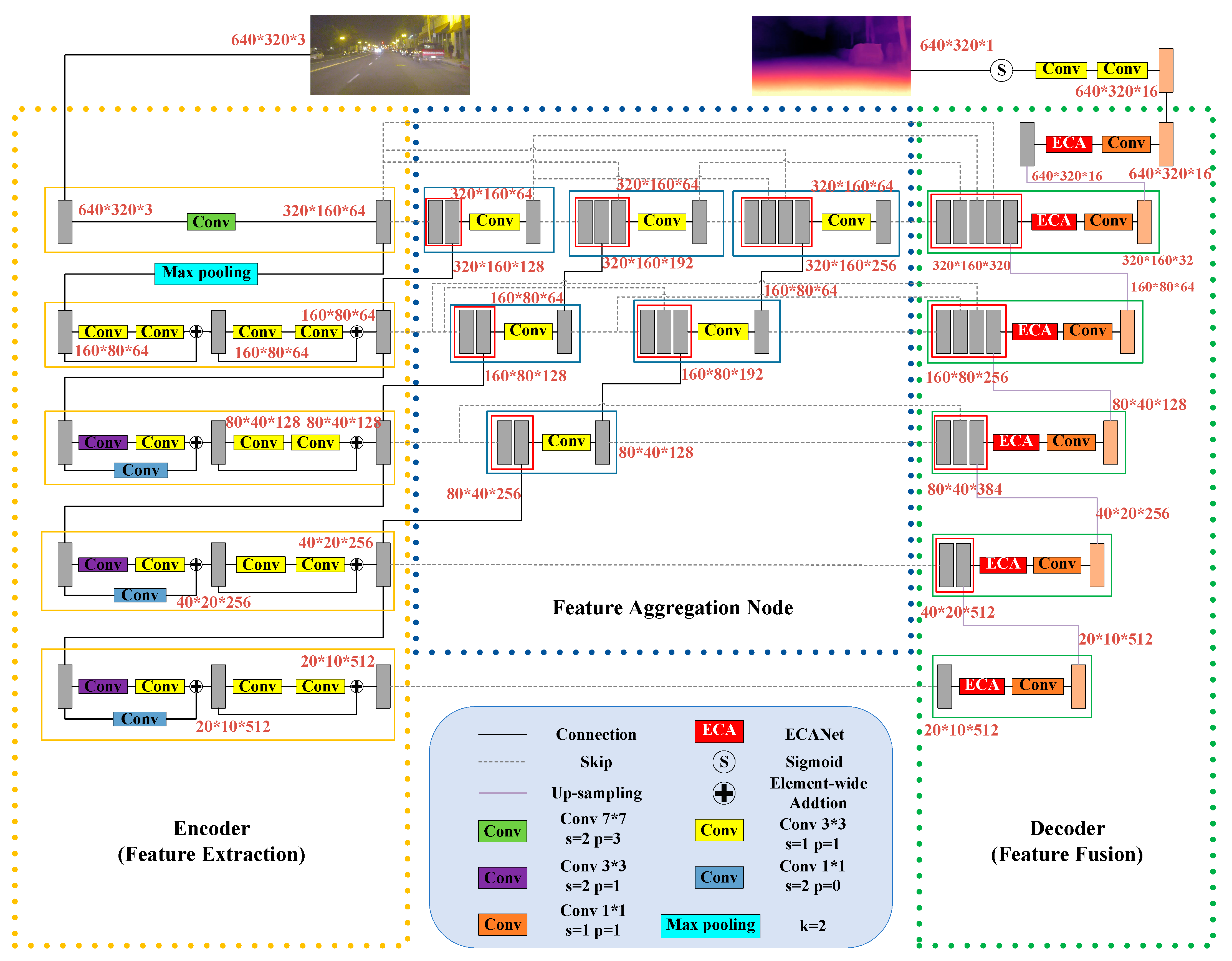
An intermediate module that incorporates multi-layer feature aggregation nodes is proposed to further integrate feature maps with varying resolutions. This module enhances the multiscale fusion effects of feature maps at different levels and helps prevent the loss of important semantic and detailed information.
(2)
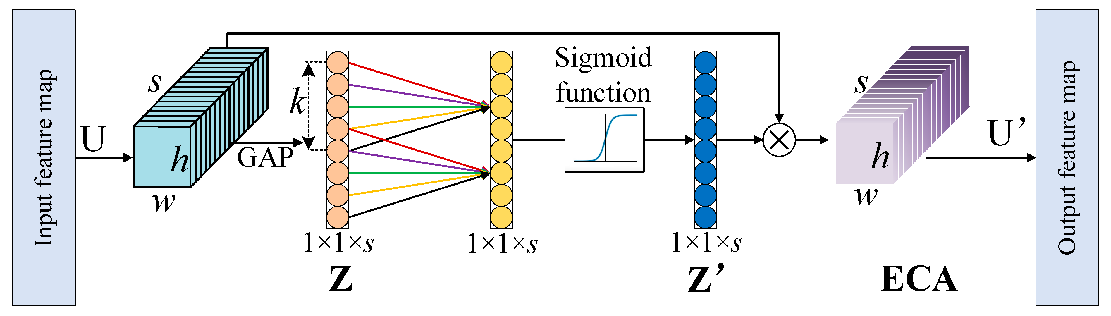
To enhance the weights of significant channels for extracting more prominent features and thereby improving the accuracy of depth estimation, the Efficient Channel Attention Module (ECANet) is integrated into the proposed network.
(3)
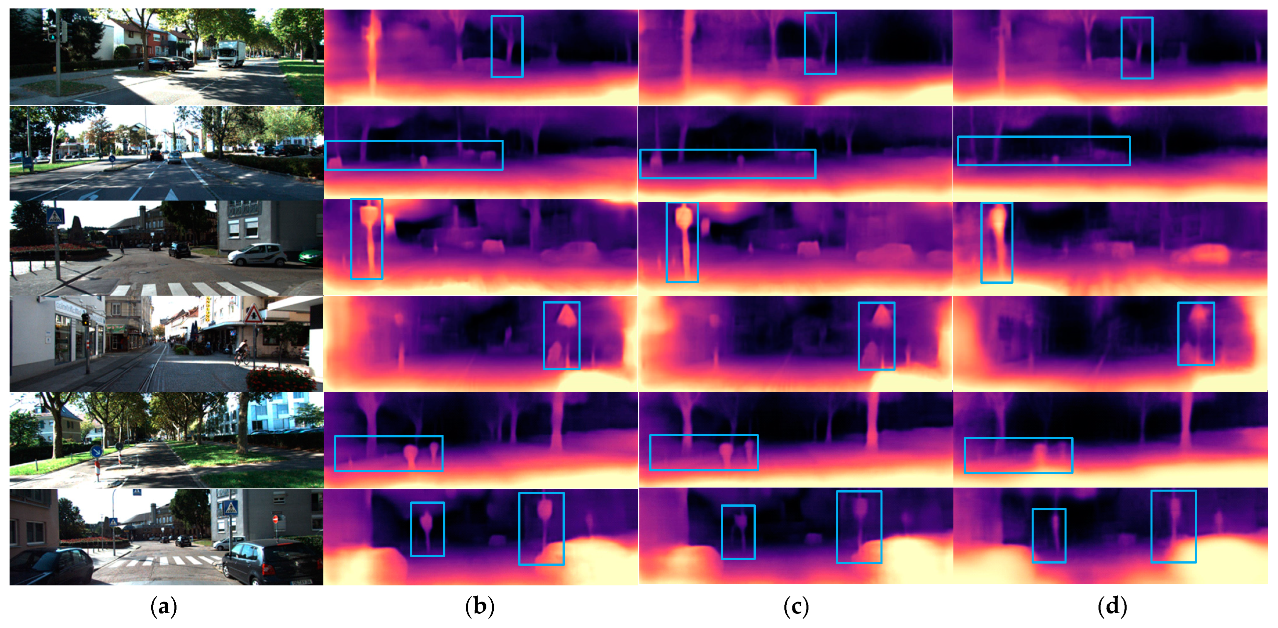
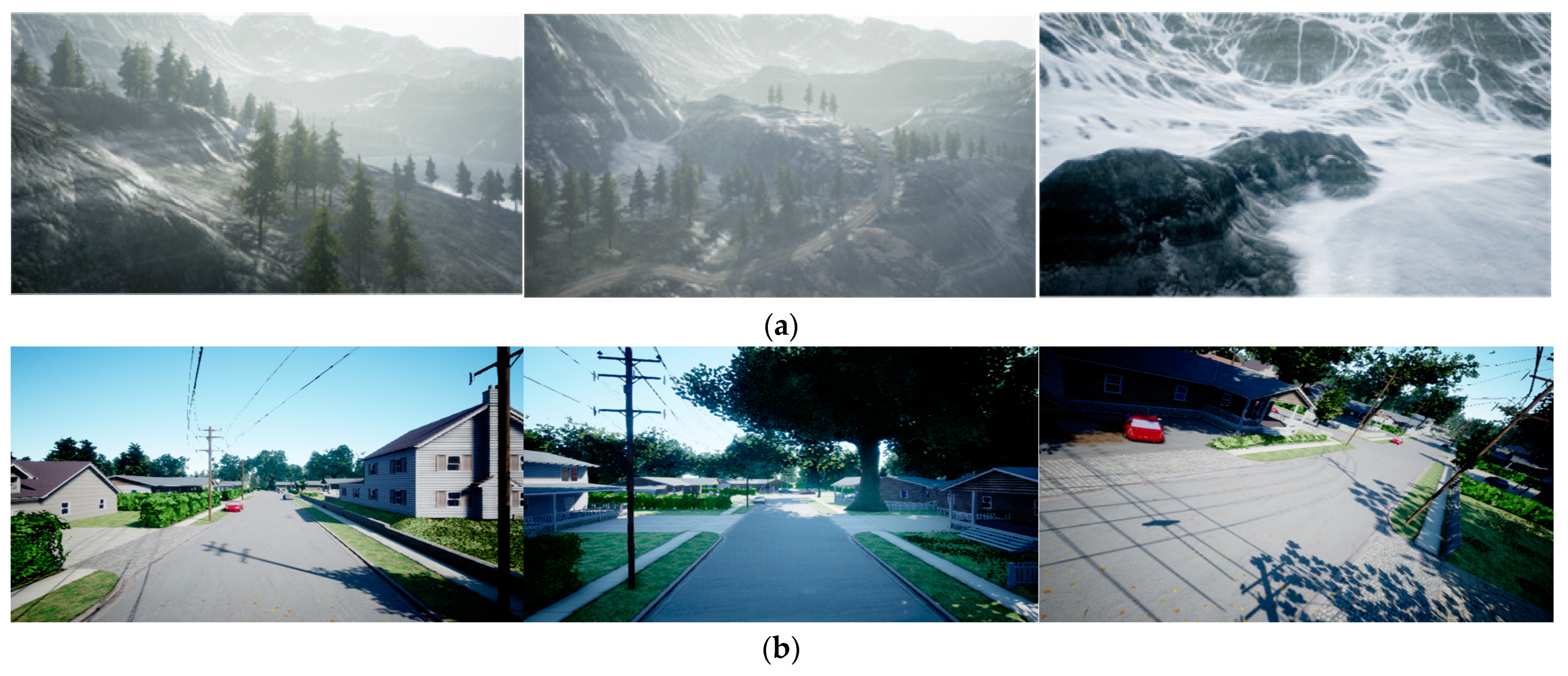
We conducted experiments using both the KITTI dataset, which was a public dataset and constructed in a real environment, and the virtual simulation dataset based on the AirSim simulation environment. These datasets encompass various lighting conditions and application scenarios. The related experimental results demonstrate that the proposed method has been initially validated and shows promising performance when compared to the original Monodepth2.
The remainder of this article is structured as follows: Section 2 presents the network architecture and innovations of our method. Section 3 outlines the experimental design and results. Finally, Section 4 concludes the article and suggests directions for future improvements.

2. Methodology

According to the pinhole camera model and stereo geometric projection, monocular depth estimation using a self-supervised learning method captures the relationships within image sequences and constructs supervised information through geometric constraints between adjacent frames. The proposed method is grounded in the principle of re-projection, with the supervisory information derived from the re-projection error, which can reveal the relationship between depth and the pose transformation of adjacent frames. Consequently, the proposed depth estimation method is a multi-task learning model that integrates both a depth estimation network and a pose estimation network.

2.1. Re-Projection

Assuming that It−1 and It are two adjacent frames, the positions of the space point P in the two camera coordinate systems are (X1, Y1, Z1) and (X2, Y2, Z2). The mathematical relation between the two position coordinates can be established by the transformation relationship existing between the two camera coordinate systems.
X 2 Y 2 Z 2 1 = R T 0 1 × 3 1 X 1 Y 1 Z 1 1
where R 3 × 3 is the rotation matrix and T 3 × 1 is the translation vector, which together is called the pose transformation matrix of the spatial point from the moment t − 1 to the moment t. The position of the spatial point P in the pixel coordinate systems in It−1 and It are denoted as (u1, v1) and (u2, v2), respectively. Based on the principle of pinhole imaging and camera intrinsic matrix K, the relationships between (u1, v1) and (X1, Y1, Z1), as well as (u2, v2) and (X2, Y2, Z2), can be established as Equation (2).
Z i u i v i 1 = [ K 0 3 × 1 ] X i Y i Z i 1 .
With the utilization of Equations (1) and (2), two equations can be derived by means of a sequence of mathematical transformations.
Z 2 u 2 v 2 1 = K R X 1 Y 1 Z 1 + K T and   X 1 Y 1 Z 1 = Z 1 K 1 u 1 v 1 1 .
According to Equation (3), (u2, v2) and Z2 can be represented as a function of K, R, T, and Z1.
Z 2 u 2 v 2 1 = Z 1 K R K 1 u 1 v 1 1 + K T .
Equation (4) is the re-projection formula. From this re-projection formula, we can find that a new image I ^ t can be reconstructed based on Equation (4) and image It-1 if the pose transformation matrix (R, T) and camera intrinsic matrix K are known. The discrepancy between the reconstructed image I ^ t and the original image It can be utilized to generate supervisory information. Therefore, the method in this paper necessitates the establishment of two separate networks for estimating the depth map and pose transformation matrix (shown in Figure 1).

2.2. Depth Estimation Network

The proposed depth estimation network is built upon the UNet++ architecture with an encoder–decoder structure [24]. The encoder extracts the detailed and semantic features by improving the model of ResNet-18. Meanwhile, the decoder transforms these features into a pixel-level depth map. Additionally, the attention mechanism ECANet is integrated into the decoder, allowing for the adjustment of weights assigned to different feature channels. This mechanism enhances the significance of important channels, facilitating the extraction of more prominent features. The overall structure of the proposed depth estimation network is illustrated in Figure 2.
In the encoder, the input image undergoes multiple down-sampling operations, as illustrated in Figure 3a, leading to a continuous reduction in the dimensions of the feature maps. During this down-sampling process, the number of channels is sequentially increased from 3 to 64, then to 128, 256, and finally 512, allowing the model to extract the high-level features. However, this process often results in the loss of crucial information that is equally important for depth estimation, such as object edges and small target regions. These areas typically suffer from low brightness and blurred textures, which makes it challenging for the model to accurately extract their feature information. The proposed method addresses this issue by incorporating multiple Feature Aggregation Nodes (FANs), as illustrated in Figure 3b, and replacing the skip connection between the encoder and decoder with FANs. This modification results in improved model performance in complex and challenging visual environments. The primary function of the FAN is to integrate multiscale features extracted from the encoder, facilitating the fusion and reuse of low-level and high-level features through intermediate nodes. This module effectively minimizes the loss of critical feature information during both down-sampling and up-sampling.
In the decoder, the high-level features extracted by the encoder are up-sampled multiple times to reduce the number of channels from 512 to 256, 128, 64, 32, and finally to 16, ultimately generating a single-channel depth map with the same resolution as the input image. The up-sampling operation of the decoder is illustrated in Figure 3c. The feature maps in the decoder are derived from the previous layer, the corresponding encoder layer, and the outputs of the FAN. Multiscale feature fusion is achieved through ECANet, which plays a crucial role in accurately extracting depth information under challenging visual conditions.

2.3. Attention Mechanism

As an effective strategy to enhance the performance of CNNs, the channel attention mechanism adjusts the weight of each channel according to its importance in relation to the features. This adjustment improves the significance of the relevant channels. The channel attention module aids the depth estimation network in extracting salient features while suppressing irrelevant ones, thereby enhancing overall performance. Currently, SENet [25] and ECANet [26] are two typical channel attention mechanisms. The primary operations of SENet involve Squeeze and Excitation, which enhance the model’s ability to perceive salient features. However, the inclusion of two fully connected layers within the SENet architecture leads to a significant increase in parameters and computational costs, as well as a heightened risk of overfitting. Additionally, the attention mechanism of SENet is based on global features, which limits its adaptability to small datasets and results in considerable performance fluctuations depending on dataset size. In contrast, ECANet addresses the limitations of SENet and has been widely adopted across various visual tasks.
The benefits of ECANet are evident in three key aspects: (1) ECANet replaces fully connected layers with multiple 1D convolutions, leading to a significant reduction in network parameters while enhancing computational efficiency. (2) ECANet employs a local cross-channel interaction strategy without dimensionality reduction, effectively capturing the interactive relationships between feature channels through 1D convolutions. This approach mitigates the negative effects of dimensionality reduction and improves the network’s feature extraction capabilities. (3) ECANet utilizes an adaptive method to adjust the size of the convolution kernel, allowing the network to accommodate feature maps of varying scales and enhancing the model’s generalization ability. Consequently, the proposed method integrates ECANet into each layer of the decoder to improve overall network performance.
As shown in Figure 4, ECANet primarily consists of global average pooling (GAP), a 1D convolution with a kernel size of 1×k, the sigmoid activation function, and other related operations. If the input feature map of ECANet is denoted as U = [ u 1 , u 2 , , u s ] h × w × s , ECANet initially conducts independent GAP on each channel.
z n = G A P ( u n ) = 1 h × w i = 1 h j = 1 w u n ( i , j )
where u n h × w represents the feature map of the channel n, GAP(·) denotes the GAP operation, and Z = [z1, z2,…, zs] 1 × 1 × s .
To capture the local cross-channel interactions, we focus on the interactions between each channel and its nearest neighbors. The channel attention weight for each channel can then be calculated using Equation (6).
Z = σ C k 1 D Z
where C k 1 D is the 1D convolution operation with a kernel size of k, σ ( ) denotes the sigmoid activation function, and Z = [ z 1 , z 2 , , z s ] is the corresponding weights of different channels.
Each element z i of the weight vector Z is multiplied by the corresponding channel ui of the input feature map U to generate a new feature map U = [ u 1 , u 2 , , u s ] . Generally, the value of k is determined by the channel number of the feature map s and can be calculated as follows [26]:
k = log 2 ( s ) + 1 2 o d d
where |·|odd means to obtain the nearest odd number from the value in parentheses.

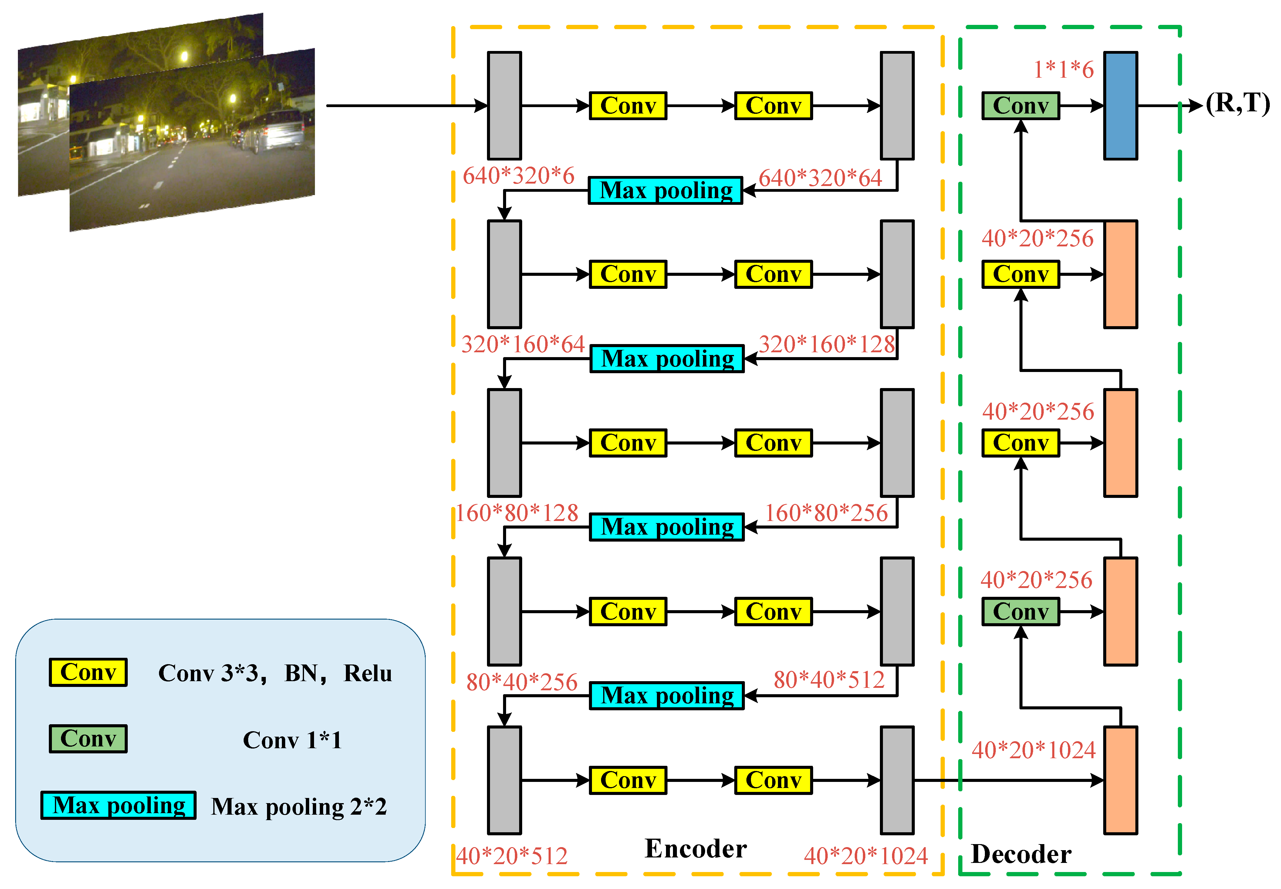
2.4. Pose Estimation Network

The pose estimation network illustrated in Figure 5 employs a CNN-based model to regress the six degrees of freedom (6-DOF) pose transformation information between two adjacent frames. This network extracts the pose transformation matrix by generating an input feature map through the superimposition of the two frames. Initially, the pose estimation network increases the number of feature map channels sequentially from 6 to 128, 256, 512, and finally 1024. It then reduces the number of feature map channels to 256 and applies two convolutional layers to extract high-level semantic features pertinent to pose transformation. Ultimately, a convolutional layer is utilized to convert the feature map into a pose transformation matrix.

2.5. Loss Function

The network model proposed in this paper consists of two processes: forward propagation and backpropagation. During the forward propagation process, the input image is reconstructed based on the output results from the depth estimation network and the pose estimation network. In the backpropagation process, the error between the reconstructed image and the original image is calculated using a loss function, which is then employed to train the network parameters. The loss function L is a weighted sum of the re-projection loss Lrep and the edge smoothing loss Lsmooth and can be expressed as follows:
L = μ L r e p + λ L s m o o t h
where μ and λ represent the weights assigned to the re-projection loss and edge smoothing loss, respectively. In the proposed method, their values are set to μ = 1 and λ = 0.04 according to the values taken by Monodepth2.
The re-projection loss Lrep can be presented as follows [27]:
L r e p = α 2 1 2 u I u J + C 1 u I 2 + u J 2 + C 1 × 2 σ I J + C 2 σ I 2 + σ J 2 + C 2 + ( 1 α ) i = 1 N j = 1 M I ( i , j ) J ( i , j )
where I is the input image, J is the image reconstructed based on the re-projection principle, and I and J have the same resolution of M × N pixels. uI and uJ denote the mean pixel value of the images I and J, respectively. σ I J is the covariance of the images I and J, and σ I and σ J are the standard deviation of pixel values of the images I and J, respectively. The constant α is generally taken to be 0.85 [27].
Using the edge smoothing loss Lsmooth can effectively mitigate depth discontinuities, suppress noise, and enhance the clarity of edges in the depth map [28]. Its mathematical formulation is presented as follows:
L s m o o t h = 1 M N i = 1 N j = 1 M D ( i , j ) e I ( i , j ) T
The number of pixels in the input image is denoted by M × N. The equation above reveals that the edge smoothing loss consists of two components: the depth smoothing term ∇D, which mitigates local singular noise in the depth map and enhances its smoothness, and the edge perception term ∇I, which promotes feature learning at edges with significant depth gradients to produce clearer contours. During the training phase, a smaller sum of ∇D and a greater amount of edge information ∇I yield better results. Consequently, Equation (10) employs negative exponential functions to ensure that both the depth smoothing term ∇D and the edge perception term ∇I change in the same direction.

3. Experiment

In this section, we conduct a series of comparative experiments to achieve the following objectives: (1) We evaluate the proposed method using the public KITTI dataset to validate its depth estimation performance for AGVs. (2) We assess the performance of the proposed method in the context of UAVs by utilizing a custom dataset generated from AirSim simulation software(https://microsoft.github.io/AirSim/, accessed on 10 April 2025), which provides ground truth for scene depth.
In our paper, performance evaluation encompasses both quantitative and qualitative comparisons. The depth estimation results at the pixel level are quantitatively assessed using seven metrics, as shown in Table 1. The variable di represents the ground truth, while d i * represents the estimated depth value. N refers to the total number of pixels in the input image.

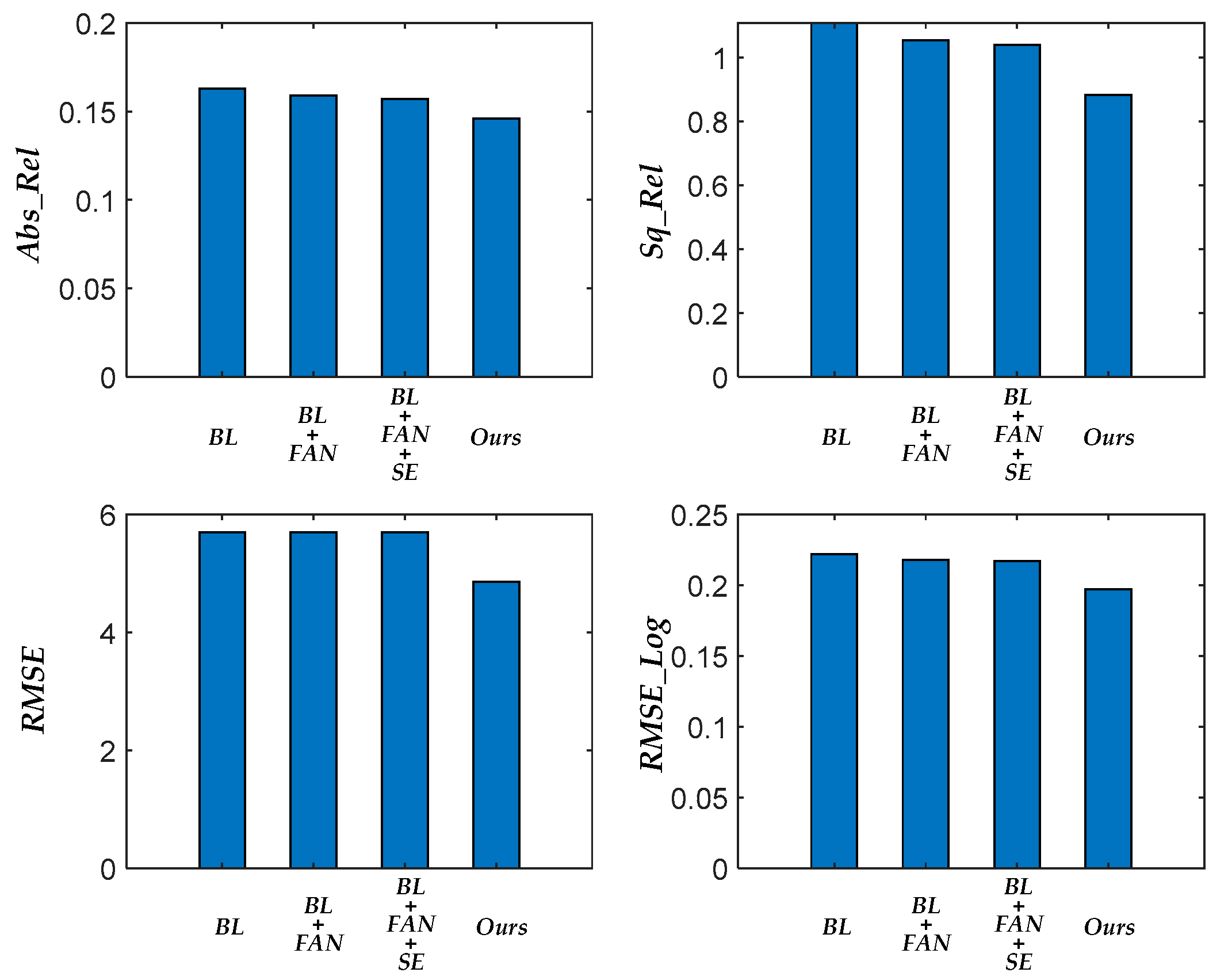
3.1. Performance Evaluation for AGVs

Dataset: The KITTI dataset is widely recognized as the most extensively utilized publicly available dataset for depth estimation. Since the videos in this dataset are captured by AGVs, we use it to test and evaluate the proposed method applied to AGVs. In this experiment, we adopt the data-splitting method proposed by Eigen et al. [19] and manually exclude the static frames, following the approach of Zhou et al. [29]. Ultimately, the training set consists of 39,810 images, the validation set contains 4424 images, and the test set comprises 697 images.
Implementation Details: The experimental platform operates on Ubuntu 20.04.5, while the neural network models are built using the PyTorch 1.7 open-source framework. The camera intrinsic matrix K is presented in Equation (11), derived from the intrinsic parameters of the acquisition used in the KITTI dataset. The workstation is equipped with an RTX 3090 Ti graphics card, and during the training process, we employ the Adam optimizer for gradient descent optimization. The model is trained for 20 epochs, with a batch size of 8 determined by the workstation’s performance. The learning rate is set to 10−4 for the first 15 epochs and is subsequently adjusted to 10−5 for the remaining 5 epochs.
K = 718.8560 0 607.1928 0 718.8560 185.2157 0 0 1
Quantitative Comparison and Evaluation: The proposed method and two other baseline methods, HR-Depth and Monodepth2, are compared using the same test sets, and the results of the comparative experiment are presented in Table 2. It can be seen that the proposed method demonstrated superior performance on the test set due to structural upgrades and the addition of ECANet, as evidenced by most indexes outperforming the two other methods.
To evaluate the impact of the first and second contributions on depth estimation performance, we conducted ablation experiments on the KITTI dataset. As previously mentioned, the contributions of this paper consist of two main components: the design of feature aggregation nodes (FANs) and the incorporation of ECANet in the decoder. Consequently, we tested four algorithms in the ablation experiments: Baseline (BL), Baseline with integrated feature aggregation nodes (BL+FAN), Baseline+FAN with the introduction of SENet in the decoder (Baseline+FAN+SE), and our proposed approach (Baseline+FAN+ECA). The results of the ablation experiments are presented in Figure 6. Based on the changes observed in the four evaluation metrics presented in Figure 6, we can draw the following conclusions: (1) Integrating feature aggregation nodes into the baseline model improves depth estimation performance to some extent; (2) the algorithm’s performance can be significantly enhanced by utilizing ECANet instead of SENet within the Baseline+FAN framework.
Qualitative Comparison and Evaluation: The depth maps of Figure 7 utilize distinct color variations to delineate the relative spatial relationships within the scene. Lighter hues indicate proximity, while darker shades signify greater distance. From Figure 7, we can observe that the proposed approach effectively captures comprehensive depth information of the scene with a relatively high degree of accuracy and accurately portrays specific targets’ spatial characteristics through color differentiation. The proposed method benefits from the optimized structure of the depth estimation network and the incorporation of ECANet, a channel attention mechanism. By comparing the regions in the blue bounding boxes in Figure 7, we can find that our method achieves more accurate retention and extraction of detailed features, leading to clearer and more precise contours and boundaries in the depth map.

3.2. Performance Evaluation for UAVs

The objective of this paper is to propose a methodology for addressing the challenge of forward-looking depth estimation in IMPs, including UAVs and AGVs. The experiment described in Section 3.1 was conducted using AGVs. Consequently, the experiments in this section will evaluate the depth estimation performance of the proposed method in UAV application scenarios. The image sequences utilized in this section were captured using AirSim, an open-source simulation platform developed by Microsoft. This platform is capable of simultaneously acquiring visible video sequences as input data and corresponding high-resolution depth information as ground truth. The experimental scenarios encompass two distinct environments: the snowy mountain scenario and the urban neighborhood scenario, with the aim of verifying the usability and robustness of the proposed method across different settings.
Dataset: The UAV flight forward-looking simulation dataset is divided into two groups based on different scenarios: (1) The sub-dataset from the snowy mountain scenario, referred to as AirSim_Mountain, contains 3986 images for training and 1453 images for testing. AirSim_Mountain features a diverse array of environmental elements, such as trees, mountains, and rivers, which contribute to its highly complex terrain characteristics. This complexity presents various challenges for the proposed method, including issues related to occlusion, height variations, and terrain irregularities. (2) In contrast to AirSim_Mountain, the UAVs in the AirSim_CityRoad sub-dataset primarily navigate along city roads, exhibiting relatively simple motion states that include only straight-line flight and turning. This sub-dataset comprises 3174 images for training and 1206 images for testing. Some samples from the UAV flight dataset are illustrated in Figure 8.
Implementation Details: Similar to the previous experiment, the experimental platform utilizes Ubuntu 20.04.5 as the operating system, while the neural network models are constructed using the PyTorch 1.7 open-source framework. The camera intrinsic matrix K of the AirSim is presented in Equation (12). During the training process, we also employ the Adam optimizer for gradient descent optimization. The model is trained for 20 epochs with a batch size of 8. The learning rate is initially set to 10−4 for the first 15 epochs and is subsequently adjusted to 10−5 for the remaining 5 epochs.
K = 320 0 320 0 359.185 240 0 0 1
Quantitative Comparison and Evaluation: Since the AirSim_Mountain and AirSim_CityRoad sub-datasets were generated with pixel-level depth labeling, the performance of depth estimation methods on the AirSim dataset can be evaluated quantitatively by directly comparing the predicted depth of each pixel with the true depth. As shown in Table 3, all assessment criteria for the proposed method significantly outperform those of the other two methods. The prediction accuracy also demonstrates a high level of performance; for instance, using Abs_Rel and thr Acc (where thr = 1.25) as examples, the proposed method reduces the error by a maximum of 7.9% and improves the accuracy by a maximum of 1.3% compared to Monodepth2, which serves as the baseline method. Therefore, the quantitative comparison results clearly demonstrate the significant performance advantage of our method in the depth estimation task, as well as the validity of the improvements and optimizations made to the network architecture in the proposed approach.
Qualitative Comparison and Evaluation: For the test results of the samples from the AirSim_Mountain dataset shown in Figure 9a, when the UAV is flying in a mountainous area, the proposed method can accurately distinguish the relative distances and proximity of obstacle targets in its path, such as trees, peaks, and rocks. Additionally, compared to the other two methods, our approach provides a more detailed analysis of contours and edge regions. Furthermore, due to the complexity of mountainous environments, texture information often introduces visual interference, such as the varying shapes of snow bands and rivers, which can easily lead to errors in judgment and negatively impact the overall accuracy of depth estimation. However, the method presented in this paper can effectively address these challenges by focusing solely on the spatial relationships within the scene while disregarding the adverse effects of texture information, thereby yielding more precise depth prediction results. It is important to note that the distant targets in the depth map have blended into the background, making it difficult to estimate their depth accurately. For the AirSim_CityRoad dataset, using four samples from Figure 9b as examples, the depth estimation method proposed in this paper demonstrates a comprehensive understanding of road structure and analyzes the geometric features of intersections. It exhibits strong depth perception capabilities in urban road scenes. Furthermore, our method accurately captures and interprets the environmental features on both sides of the road, particularly objects such as trees, lampposts, and road signs. It effectively represents the spatial locations and distances of these targets in depth maps, thereby addressing the visual challenges presented by complex road scenes.
Under the same experimental conditions, we have evaluated the inference speed of the proposed method using images at two resolutions. For images sized 384 × 192 pixels and 640 × 320 pixels, the inference speeds were 56.3 frames per second (FPS) and 40.8 FPS, respectively. For real-time applications, the proposed method achieves a reasoning speed exceeding 40 FPS for images sized 640 × 320 pixels. However, the majority of civil IMPs currently in use support a video frame rate of approximately 30 FPS. Consequently, our method can achieve real-time inference for depth estimation.

4. Conclusions

To address the demands of depth estimation in various environments for IMPs, we propose a novel method for monocular depth estimation based on self-supervised learning. Our approach incorporates an intermediate module between the encoder and decoder of the depth estimation network, facilitating cross-level feature fusion. Additionally, we integrate ECANet into the depth estimation network to enhance accuracy by increasing the weights of significant channels, allowing for the extraction of more prominent features and improving the retention of semantic information in the results. Experimental results demonstrate that our method is well-suited for depth estimation across diverse environmental conditions. Furthermore, it shows that the proposed approach outperforms baseline methods in both real-world and simulated scenarios.
Nevertheless, some challenges persist regarding our method. Firstly, the model exhibits limited generalization ability due to the absence of large-scale training and testing datasets. Currently, the available datasets for depth estimation are primarily sourced from ground platforms and lack pixel-level dense ground truth, which poses a challenge for achieving quantitative evaluation. Secondly, there remains a significant gap when compared to active sensors such as LIDAR. Therefore, it is beneficial to explore the joint application of vision sensors with other technologies, such as inertial navigation and radar, to facilitate mutual learning. Moreover, integrating the depth map generated by the depth estimation algorithm with semantic or instance segmentation algorithms can complete distance measurements to specific targets within an image. This is one of the key areas we are currently exploring.

Author Contributions

Conceptualization, L.W. and M.D.; methodology, L.W.; software, S.L.; validation, L.W. and S.L.; data curation, S.L.; writing—original draft preparation, L.W.; writing—review and editing, L.W. and S.L.; visualization, L.W.; supervision, M.D.; project administration, M.D.; funding acquisition, M.D. All authors have read and agreed to the published version of the manuscript.

Funding

This work was supported by the National Natural Science Foundation of China (No. U2433207 and U2033201), the Aeronautical Science Foundation of China (No. 20220058052001), and the School-level Research Fund Project of Nanhang Jincheng College (No. XJ202307).

Institutional Review Board Statement

Not applicable.

Informed Consent Statement

Not applicable.

Data Availability Statement

The proposed algorithm and datasets in this paper can be obtained by contacting the corresponding author of this paper (nuaa_dm@nuaa.edu.cn).

Acknowledgments

All individuals included in this section have consented to the acknowledgement.

Conflicts of Interest

The authors declare no conflict of interest.

References

  1. Wang, Y.; Wang, J.; Zhang, W.; Zhan, Y.; Guo, S.; Zheng, Q.; Wang, X. A survey on deploying mobile deep learning applications: A systemic and technical perspective. Digit. Commun. Netw. 2022, 8, 1–7. [Google Scholar] [CrossRef]
  2. Gong, T.; Zhu, L.; Yu, F.R.; Tang, T. Edge intelligence in intelligent transportation systems: A survey. IEEE Trans. Intell. Transp. Syst. 2023, 24, 8919–8944. [Google Scholar] [CrossRef]
  3. Raj, R.; Kos, A. A comprehensive study of mobile robot: History, developments, applications, and future research perspectives. Appl. Sci. 2022, 12, 6951. [Google Scholar] [CrossRef]
  4. Yeong, D.J.; Velasco-Hernandez, G.; Barry, J.; Walsh, J. Sensor and sensor fusion technology in autonomous vehicles: A review. Sensors 2021, 21, 2140. [Google Scholar] [CrossRef] [PubMed]
  5. Milburn, L.; Gamba, J.; Fernandes, M.; Semini, C. Computer-Vision Based Real Time Waypoint Generation for Autonomous Vineyard Navigation with Quadruped Robots. In Proceedings of the 2023 IEEE International Conference on Autonomous Robot Systems and Competitions, Tomar, Portugal, 26–27 April 2023; pp. 239–244. [Google Scholar]
  6. Chen, L.; Li, Y.; Huang, C.; Li, B.; Xing, Y.; Tian, D.; Li, L.; Hu, Z.; Na, X.; Li, Z.; et al. Milestones in autonomous driving and intelligent vehicles: Survey of surveys. IEEE Trans. Intell. Veh. 2022, 8, 1046–1056. [Google Scholar] [CrossRef]
  7. Lu, Y.; Xue, Z.; Xia, G.S.; Zhang, L. A survey on vision-based UAV navigation. Geo-Spat. Inf. Sci. 2018, 21, 21–32. [Google Scholar] [CrossRef]
  8. Opromolla, R.; Fasano, G. Visual-based obstacle detection and tracking, and conflict detection for small UAS sense and avoid. Aerosp. Sci. Technol. 2021, 119, 107167. [Google Scholar] [CrossRef]
  9. Zhang, C.; Cao, Y.; Ding, M.; Li, X. Object depth measurement and filtering from monocular images for unmanned aerial vehicles. J. Aerosp. Inf. Syst. 2022, 19, 214–223. [Google Scholar] [CrossRef]
  10. Wang, Y.; Chao, W.L.; Garg, D.; Hariharan, B.; Campbell, M.; Weinberger, K.Q. Pseudo-lidar from visual depth estimation: Bridging the gap in 3d object detection for autonomous driving. In Proceedings of the 2019 IEEE/CVF Conference on Computer Vision and Pattern Recognition (CVPR), Long Beach, CA, USA, 15–20 June 2019; pp. 8445–8453. [Google Scholar]
  11. Fan, L.; Wang, J.; Chang, Y.; Li, Y.; Wang, Y.; Cao, D. 4D mm Wave radar for autonomous driving perception: A comprehensive survey. IEEE Trans. Intell. Veh. 2024, 9, 4606–4620. [Google Scholar] [CrossRef]
  12. Zhao, C.; Sun, Q.; Zhang, C.; Tang, Y.; Qian, F. Monocular depth estimation based on deep learning: An overview. Sci. China Technol. Sci. 2020, 63, 1612–1627. [Google Scholar] [CrossRef]
  13. Deliry, S.I.; Avdan, U. Accuracy of unmanned aerial systems photogrammetry and structure from motion in surveying and mapping: A review. J. Indian Soc. Remote Sens. 2021, 49, 1997–2017. [Google Scholar] [CrossRef]
  14. Zhang, Y.; Wu, Y.; Tong, K.; Chen, H.; Yuan, Y. Review of visual simultaneous localization and mapping based on deep learning. Remote Sens. 2023, 15, 2740. [Google Scholar] [CrossRef]
  15. Mertan, A.; Duff, D.J.; Unal, G. Single image depth estimation: An overview. Digit. Signal Process. 2022, 123, 103441. [Google Scholar] [CrossRef]
  16. Poggi, M.; Tosi, F.; Batsos, K.; Mordohai, P.; Mattoccia, S. On the synergies between machine learning and binocular stereo for depth estimation from images: A survey. IEEE Trans. Pattern Anal. Mach. Intell. 2021, 44, 5314–5334. [Google Scholar] [CrossRef] [PubMed]
  17. Masoumian, A.; Rashwan, H.A.; Cristiano, J.; Asif, M.S.; Puig, D. Monocular depth estimation using deep learning: A review. Sensors 2022, 22, 5353. [Google Scholar] [CrossRef] [PubMed]
  18. Dong, X.; Garratt, M.A.; Anavatti, S.G.; Abbass, H.A. Towards real-time monocular depth estimation for robotics: A survey. IEEE Trans. Intell. Transp. Syst. 2022, 23, 16940–16961. [Google Scholar] [CrossRef]
  19. Eigen, D.; Puhrsch, C.; Fergus, R. Depth map prediction from a single image using a multi-scale deep network. In Proceedings of the 2014 Advances in Neural Information Processing Systems, Montreal, QC, Canada, 8–13 December 2014; p. 27. [Google Scholar]
  20. Liu, F.; Shen, C.; Lin, G. Deep convolutional neural fields for depth estimation from a single image. In Proceedings of the 2015 IEEE Conference on Computer Vision and Pattern Recognition (CVPR), Boston, MA, USA, 7 June 2015; pp. 5162–5170. [Google Scholar]
  21. Huang, B.; Zheng, J.Q.; Nguyen, A.; Tuch, D.; Vyas, K.; Giannarou, S.; Elson, D.S. Self-supervised generative adversarial network for depth estimation in laparoscopic images. In Proceedings of the 24th International Conference on Medical Image Computing and Computer Assisted Intervention, Strasbourg, France, 27 September–1 October 2021; pp. 227–237. [Google Scholar]
  22. Godard, C.; Mac Aodha, O.; Firman, M.; Brostow, G.J. Digging into self-supervised monocular depth estimation. In Proceedings of the 2019 IEEE/CVF International Conference on Computer Vision, Seoul, Republic of Korea, 27 October–2 November 2019; pp. 3828–3838. [Google Scholar]
  23. Liu, J.; Kong, L.; Yang, J.; Liu, W. Towards better data exploitation in self-supervised monocular depth estimation. IEEE Robot. Autom. Lett. 2023, 9, 763–770. [Google Scholar] [CrossRef]
  24. Zhou, Z.; Rahman Siddiquee, M.M.; Tajbakhsh, N.; Liang, J. Unet++: A nested u-net architecture for medical image segmentation. In Proceedings of the Deep Learning in Medical Image Analysis and Multimodal Learning for Clinical Decision Support: 4th International Workshop, Granada, Spain, 20 September 2018; pp. 3–11. [Google Scholar]
  25. Hu, J.; Shen, L.; Sun, G. Squeeze-and-excitation networks. In Proceedings of the 2018 IEEE Conference on Computer Vision and Pattern Recognition, CVPR 2018, Salt Lake City, UT, USA, 18–22 June 2018; pp. 7132–7141. [Google Scholar]
  26. Wang, Q.; Wu, B.; Zhu, P.; Li, P.; Zuo, W.; Hu, Q. ECA-Net: Efficient channel attention for deep convolutional neural networks. In Proceedings of the 2020 IEEE/CVF Conference on Computer Vision and Pattern Recognition, Seattle, WA, USA, 14–19 June 2020; pp. 11534–11542. [Google Scholar]
  27. Wang, Z.; Bovik, A.C.; Sheikh, H.R.; Simoncelli, E.P. Image quality assessment: From error visibility to structural similarity. IEEE Trans. Image Process. 2004, 13, 600–612. [Google Scholar] [CrossRef] [PubMed]
  28. Seif, G.; Dimitrios, A. Edge-Based Loss Function for Single Image Super-Resolution. In Proceedings of the 2018 IEEE International Conference on Acoustics, Speech and Signal Processing (ICASSP), Calgary, AB, Canada, 15–20 April 2018; pp. 1468–1472. [Google Scholar]
  29. Zhou, T.; Brown, M.; Snavely, N.; Lowe, D.G. Unsupervised learning of depth and ego-motion from video. In Proceedings of the 2017 IEEE Conference on Computer Vision and Pattern Recognition, Honolulu, HI, USA, 21–26 July 2017; pp. 1851–1858. [Google Scholar]
Figure 1. The framework of the proposed approach.
Applsci 15 04267 g001
Figure 2. The structure of the depth estimation network proposed in this paper.
Applsci 15 04267 g002
Figure 3. Components of the depth estimation network. (a) Down-sampling operations with convolution in the encoder. (b) Feature aggregation nodes. (c) Up-sampling operations with ECA in the decoder.
Applsci 15 04267 g003
Figure 4. The structure of ECANet.
Applsci 15 04267 g004
Figure 5. The structure of the pose estimation network.
Applsci 15 04267 g005
Figure 6. Comparison of the four evaluation metrics in ablation experiments on the KITTI dataset.
Applsci 15 04267 g006
Figure 7. The results of qualitative comparison based on the KITTI dataset. (a) Test images. (b) The proposed method. (c) HR-Depth. (d) Monodepth2.
Applsci 15 04267 g007
Figure 8. Samples from the Airsim datasets. (a) AirSim_Mountain. (b) AirSim_CityRoad.
Applsci 15 04267 g008
Figure 9. The results of qualitative comparison based on the AirSim datasets. (a) Results from AirSim_Mountain. (b) Results from AirSim_CityRoad.
Applsci 15 04267 g009
Table 1. Quantitative evaluation metrics.
Evaluation IndexFormula
Absolute relative error
Abs Rel
1 N i = 1 N d i d i d i
Square relative error
Sq Rel
1 N i = 1 N d i d i 2 d i
Root mean square error
RMSE
1 N i = 1 N d i d i 2
Root mean square logarithmic error
RMSE log
1 N i = 1 N log d i log d i 2
Threshold
accuracy
max d i d i , d i d i = δ < t h r
thr Accthr = 1.25, 1.252, 1.253
Table 2. The results of quantitative comparison based on the KITTI dataset (The best result in each column is shown in bold).
MethodAbs_RelSq_RelRMSERMSE_LogThr Acc (thr = 1.25)Thr Acc (thr = 1.252)Thr Acc (thr = 1.253)
Proposed0.1460.8834.8570.1970.7920.9540.988
HR-Depth0.1571.0395.6980.2170.7510.9410.985
Monodepth20.1631.1085.6990.2220.7500.9310.982
Table 3. The results of quantitative comparison based on the AirSim simulation dataset. (The best result in each column in each sub-dataset is shown in bold).
Test SampleMethodAbs_RelSq_RelRMSERMSE_LogThr Acc (thr = 1.25)Thr Acc (thr = 1.252)Thr Acc (thr = 1.253)
AirSim_MountainProposed0.2111.2415.4930.3210.7830.9430.982
HR-Depth0.2181.3925.8640.3950.7710.9400.979
Monodepth20.2291.5036.1040.4610.7730.9240.978
AirSim_CityRoadProposed0.2421.3645.7900.3550.7790.9420.980
HR-Depth0.2531.4725.9410.4320.7760.9410.978
Monodepth20.2561.5776.0770.5150.7720.9390.977
Disclaimer/Publisher’s Note: The statements, opinions and data contained in all publications are solely those of the individual author(s) and contributor(s) and not of MDPI and/or the editor(s). MDPI and/or the editor(s) disclaim responsibility for any injury to people or property resulting from any ideas, methods, instructions or products referred to in the content.

