Article

An Artificial Plant Community Algorithm for Collision-Free Multi-Robot Aggregation

Hubei Province Engineering Technology Research Center for Construction Quality Testing Equipments, College of Computer and Information Technology, China Three Gorges University, Yichang 443002, China
*
Author to whom correspondence should be addressed.
Appl. Sci. 2025, 15(8), 4240; https://doi.org/10.3390/app15084240
Submission received: 20 February 2025 / Revised: 8 April 2025 / Accepted: 9 April 2025 / Published: 11 April 2025

Abstract

:
Multi-robot aggregation is an important application for emergent robotic tasks, in which multiple robots are aggregated to work collaboratively. In this context, the collision-free problem poses a significant challenge, which is complicated to resolve, as aggregated robots are prone to collision. This study attempts to use robotic edge intelligence technology to solve this problem. First, a multiple objective function is built for the collision-free multi-robot aggregation problem, considering the characteristics of robotic aggregation and collision-free constraints. Second, a heuristic artificial plant community algorithm is proposed to obtain an optimal solution to the developed problem model, which is lightweight and can be deployed on edge robots to search for the optimal route in real-time. The proposed algorithm utilizes the swarm learning capability of edge robots to produce a set of collision-free aggregation assignments for all robots. Finally, a benchmark test set is developed, based on which a series of benchmark tests are conducted. The experimental results demonstrate that the proposed method is effective and its computational performance is suitable for robot edge computing.

1. Introduction

Due to their good mobility and fatigue resistance, various robots and unmanned aerial/ground vehicles—such as robotic arms, auto-guided vehicles (AGVs), unmanned aerial vehicles (UAVs), and unmanned surface vehicles (USVs)—have been widely used to replace humans in carrying out dangerous and complex tasks [1]. Collaboration and aggregation among multiple robots often provide advantages that cannot be achieved with a single robot [2]. However, collisions are also prone to occur during the aggregation of various robots. The collision-free multi-robot aggregation problem (CMAP) is a significant challenge that arises in many real-world applications. To address the CMAP, multiple robots must be assigned in an optimal manner to implement geographically distributed tasks collaboratively while avoiding collisions and ensuring a minimal makespan (i.e., the completion time of the last task) [3]. In many security and rescue applications, multiple robots are often required, and consideration of the CMAP can allow for optimized assignments, instructing the robots to aggregate to achieve important goals while simultaneously avoiding collisions. For example, when facing a fire, it is often necessary for a swarm of robots to aggregate and carry out firefighting tasks on important fire sources, as serious fires can cause huge losses of life and property [1,3].
However, finding the global optimal solution to the CMAP is not an easy task, making the CMAP a challenging issue. For example, the emergence of a task is random, chaotic, and unpredictable [1,4], and it is generally impossible to know in advance where the next emergency task will appear in large-scale firefighting and disaster rescue situations. Popular methods often divide the CMAP into two sub-problems: the multi-robot aggregation problem [5] and the collision-free multi-robot problem [6]. In each sub-problem, collaboration between multiple robots allows each task to be assigned to various robots, expanding the search space to that of non-collaborative task assignment problems [7]. In a dynamic scenario, multiple robots search for the goals to complete tasks, and more robots can dynamically aggregate to execute the emergent missions. A tiny disturbance in the solution process may produce a different makespan; therefore, the CMAP is NP-hard and requires too high of a computational cost to be effectively solved in real time.
To address this complicated problem, researchers have developed many methods to guide the activities of robots. Heuristic algorithms often achieve near-optimal results in a very short time and are considered promising for the execution of multi-robot system missions; such algorithms include grey wolf optimization (GWO) [2], the genetic algorithm (GA) [3], particle swarm optimization (PSO) [4], fuzzy logic (FL) [5,6], ant colony optimization (ACO) [7], deep learning (DL) [8], and reinforcement learning (RL) [9]. In the CMAP context, any delay in a task may result in a large aggregation of emergent tasks, making the solution space very rugged. The following emergent tasks are not yet detected by most robots, as they have not arrived at this point. Artificial intelligence-based approaches [10] can effectively help to allocate the task to a suitable robot through the analysis and synthesis of environmental information and task data.
However, most studies focused on the CMAP have separately focused on aggregation or collision, where the aggregation and collision information are not integrated [11]. If only an optimal solution for the aggregation problem or collision problem is obtained, it may be impossible to obtain an optimal solution to the global problem [12,13]. Additionally, traditional solution methods and heuristic algorithms cannot efficiently search for all solutions in uncertain environments [14,15]. When an emergent task is detected, it is difficult to modify the pre-planned solution to re-assign all tasks. Our research motivation is to solve the CMAP efficiently. For this purpose, a robotic edge intelligence (REI) architecture [10] is established, a multi-objective CMAP function is designed, a novel swarm search algorithm is proposed, and a CMAP benchmark test set is developed.
This article provides the following contributions:
First, a multi-objective CMAP function is designed that integrates the makespan, collision time, energy consumption, and total distance with battery capacity constraints for collision-free multi-robot aggregation problems. The aggregation problem and the collision-free problem are integrated while considering time-varying tasks, collaboration between robots, and dynamic environments.
Second, a novel heuristic algorithm is proposed, which can be deployed on edge robots to efficiently handle the dynamic relationships between robots and tasks. The algorithm is improved on the basis of an artificial plant community (APC) [16,17], has low hardware requirements and simple parameters, and can be run on the embedded robotic platforms.
Third, a CMAP benchmark set is developed and investigated based on references [18] and [19], which takes the characteristics of the collision-free multi-robot aggregation problem into consideration, including the number of robots and tasks, dynamic processing time, and travel time.
The remainder of this article is organized as follows. Section 2 reviews the related work. Section 3 illustrates the REI architecture. Section 4 builds a multi-objective model for solving the CMAP. Afterward, the proposed APC algorithm is introduced in Section 5. Section 6 presents the benchmark set and experimental studies. Finally, the conclusions are drawn in Section 7.

2. Related Work

This section introduces the related work on the collision-free multi-robot aggregation problem. In automated production lines for complex products, multiple robots often need to gather together to simultaneously complete collaborative processing tasks that cannot be completed by a single robot [8]. In a smart warehousing system, different logistics robots often aggregate in a certain area for simultaneous loading and unloading. In a benchmark test, we also demonstrated a scenario of multi-robot collaborative processing in a real factory [11]. The CMAP is a kind of combinational optimization problem that integrates various factors in relation to both robots and tasks. The related literature can be divided into two categories, namely, studies focused on the multi-robot aggregation problem or studies on the collision-free multi-robot problem.

2.1. Multi-Robot Aggregation Problem

Due to the fact that collaboration between multiple robots can greatly improve work efficiency and allows for the completion of tasks that a single robot cannot handle, multi-robot systems have begun to be widely applied, leading to the emergence of the multi-robot aggregation problem. An aggregation of multiple robots can form swarm intelligence that a single robot does not possess, while the failure of one or several of the robots will not affect the normal operation of the entire multi-robot system [2].
To solve the multi-robot aggregation problem, one must determine how to assign multiple robots to multiple tasks in a way that optimizes the scheduling performance of the multi-robot system. Many researchers have proposed a variety of methods to address the multi-robot aggregation problem, which can be categorized into static coordination strategies and dynamic methods.
First, static coordination strategies involve pre-arranging multiple robots to coordinate and execute each task simultaneously. A recruitment coordination strategy is a commonly used method to address the multi-robot aggregation problem through robot recruitment. If the business increment of a task is greater than the ability of the assigned robot and the robot cannot complete the task alone, more robots will be aggregated to complete the task collaboratively. In [20], a mobile federated learning approach with unreliable participants and selective aggregation was proposed. Static coordination strategies often require an integrated coordination center to provide a theoretically optimal task assignment for the small-scale static multi-robot aggregation problem, where many factors are ignored. Integrated coordination strategies allow for the pre-generation of a task assignment within a short time [21]. As these strategies do not consider the dynamic task environment during the task implementation process, they may become ineffective in many dynamic scenarios, such as fire extinguishing and earthquake rescue. Therefore, the quality of the pre-planned solutions under static coordination strategies may not meet the actual dynamic needs.
Therefore, dynamic methods employ real-time searches to obtain a good balance between makespan and the workloads of robots. The multi-man–robot problem is often modeled as a mixed-integer programming (MIP) model [22], which cannot be solved in advance. Dynamic algorithms do not require manual intervention during the task scheduling process and can obtain near-optimal solutions in a relatively limited time; such algorithms include the GA [3], FL [5,6], RL [9], and flocking-based self-organized aggregation [15]. Dynamic methods can be applied in many uncertain scenarios, where each distributed node can dynamically produce a feasible task assignment to balance the makespan of all tasks. These dynamic algorithms often employ a heuristic search mechanism to obtain good performance when solving the multi-robot aggregation problem [23]. However, the search behaviors of heuristic algorithms often lead to their premature limitation to local optimal solutions. As such, it is difficult to apply them to adjust the solution according to the dynamic task environment in real time.

2.2. Collision-Free Multi-Robot Problem

The collision-free multi-robot problem is another major challenge for multi-robot systems. When a large number of robots work together in collaboration, due to their high mobility, the avoidance of collisions and conflicts is a problem that must be considered.
One method involves installing various sensors, video surveillance devices, and radars on robots, thus enhancing their ability to perceive the environment and reduce collisions and conflicts [11,24]. With the help of various sensors, the IoT, and remote communication technologies, multiple robots can be applied to carry out tasks in unknown environments and high-risk instances.
Another method involves performing path planning and re-planning for robots, ensuring that the running routes or topologies of different robots do not collide or conflict [19]. In a dynamic environment, the obstacles or robots cannot be known until they are detected. Then, a re-planned route is generated for the robot in order to adaptively avoid obstacles, with this process being carried out in real time. In [25], a model-free visual servo swarming method for manned USVs considering visibility maintenance and collision avoidance was proposed. Heuristic algorithms—such as the artificial bee colony (ABC) algorithm [18], model–reference reinforcement learning [24], the A*-based co-evolutionary approach [26], the whale optimization algorithm (WOA) [27], and PSO [4]—can efficiently generate new routes to prevent collision and conflicts in a swarm of robots. Due to the inherent flaws of various algorithms, scholars have proposed hybrid algorithms that integrate the characteristics of different algorithms and demonstrate significant advantages, such as the fuzzy adaptive WOA [27], an ACO–ABC hybrid algorithm [28], and the WOA-AGA algorithm [29].

2.3. Collision-Free Multi-Robot Aggregation

The collision-free multi-robot aggregation problem has become a popular and interesting challenge over the past few years, with it integrating both the multi-robot aggregation problem and the collision-free multi-robot problem. The difficulty of solving this problem is higher than solving any of its sub-problems [30].
Some researchers have modeled the CMAP as a job–shop scheduling problem (JSP) with transportation [18,21]; however, there are some differences between these problem types, as shown in Table 1. As the complex relationships among robots and tasks are time-varying and dynamic, coordinated aggregation execution and collision avoidance are challenging to achieve.
As we can see from Table 1, the JSP is a scheduling problem for fixed machines and moving vehicles, while the CMAP is a scheduling problem involving fixed tasks and moving robots. In JSP with transportation, aggregation and collision issues exist between vehicles instead of machines; however, in CMAP, aggregation and collision issues between robots must be considered. In real applications, the movement of robots is dynamic and random, such that aggregation problems often lead to collision problems (and vice versa). Therefore, the optimal solutions to each of the sub-problems are generally not the optimal solution to the global problem, while dynamic task arrivals make aggregation and collision problems intertwined and difficult to separate. This problem is NP-hard and, so, manually solving the CMAP is very difficult.
In the existing literature on the CMAP, there are some research gaps. First, there is no suitable model that can effectively integrate the two sub-problems [31,32]. High expertise and domain knowledge are required to solve the CMAP, but different scenarios may produce different requirements. Second, there is no solution algorithm that can be efficiently run on embedded robotic platforms for edge computing; furthermore, the existing solution algorithms easily fall into local optima. Third, the performance of existing approaches often deteriorates sharply as the scale of the problem increases. In particular, a tiny delay in a task may lead to a much larger makespan for the other tasks, which may lead to serious issues in large-scale multi-robot systems [31]. Fourth, there is no appropriate benchmark set that can be used to test the performance of methods designed to assess the CMAP.
Our research work aims to help fill these gaps. To the best of our knowledge, no similar method has been developed to solve the collision-free multi-robot aggregation problem.

3. A Robotic Edge Intelligence Architecture

This section first describes the robotic edge intelligence architecture for the collision-free multi-robot aggregation problem, including the state transition diagrams of tasks and robots.

3.1. System Architecture

The proposed robotic edge intelligence architecture for collision-free multi-robot aggregation is depicted in Figure 1. There are two layers: the edge server layer (ESL) and the edge robot layer (ERL). In the edge server layer, there is a cloud center with many cloud servers that act as the edge servers; meanwhile, in the edge robot layer, there are many tasks and robots (e.g., robotic arms, AGVs, UAVs, and USVs).
The edge server layer provides top-layer optimization for the edge robot layer, with various edge servers integrated into the cloud center. Each robot entity in the ERL can be mapped to a virtual objective in the ESL, ensuring efficient task scheduling. Each edge server has a strong capability to perform edge computing, edge storage, communication, and artificial intelligence-based operations. It assigns all tasks to suitable robots when the tasks are accepted. In REI-based multi-robot systems, the ESL determines the fitness function and performs route planning, collision avoidance, robot aggregation, and performance optimization. When assigning tasks to a robot swarm, users need to specify the fitness function of the task in the ESL. Users can also interact with the robots in real-time and adjust the fitness function in a timely manner, based on the actual needs and progress during task execution. The edge servers can pre-arrange the robots’ routes to avoid collisions, balance the tasks between different robot swarms, and optimize operational performance before aggregation of the edge robots. The edge servers can communicate with edge robots and offload computing tasks between them, and the cloud center can complete more complex tasks that an edge robot cannot implement.
The edge robot layer includes many edge robots with edge computing and edge storage capabilities, including sensing, communication, motion control, and artificial intelligence. Each robot (e.g., robotic arm, unmanned aerial vehicle, auto guided vehicle, and unmanned surface vehicle) possesses an on-board processor as an embedded processing center. They can be mapped to the cloud center for task scheduling and can offload edge computing tasks to each other. Multiple robots can work in a coordinated manner to implement more complex tasks, such as collision avoidance and aggregation. Multiple robots perceive and share the external environment through a variety of sensors and communication technology and upload task and vehicle states to the ESL. Artificial intelligence on edge servers and edge robots allows for the formation of swarm intelligence, enabling the efficient processing of state information and optimized collision-free multi-robot aggregation.
Regarding engineering applications, some suggestions have been made for the robotic edge intelligence architecture in order to solve the collision-free multi-robot aggregation problem.
First, the edge servers and edge robots can be isomorphic or heterogeneous. The edge servers can be existing servers in production management systems, providing stronger edge computing capacity, operation rules, and objective functions. The edge robots utilize embedded platforms and on-board sensors to provide context awareness.
Second, the robotic edge intelligence architecture can be decentralized for the implementation of various tasks. Edge servers and edge robots have equal status and can offload computing tasks to each other. To fully utilize their powerful computing capacity, edge servers are often allocated to more complex computing tasks that an edge robot cannot complete.
Third, the distributed collaboration of edge servers and robots allows for the formation of swarm intelligence. The edge computing capacity and the artificial intelligence module are designed to ensure that the REI system can solve the collision-free multi-robot aggregation problem in real time. The computational cost and delay can be greatly reduced, and the computing power increases as the number of robots increases.
Fourth, the edge server layer serves as the virtual layer in the REI architecture, while the edge robot layer serves as the physical layer. They are connected by communication devices and protocols, such that a physical robot in the ERL can be mapped to a virtual robot in the ESL, while a virtual robot in the ESL can schedule a physical robot in the ERL. Task and robot scheduling is carried out based on the state transition diagrams described in the following subsection.

3.2. State Transition Diagram of Tasks

As mentioned above, an accurate scheduling model is important to apply an REI-based multi-robot system, where the design of the model depends on the states of the tasks and robots. The state transitions can help to instruct the REI-based multi-robot system, allowing it to assign tasks to appropriate robots. The state transition diagrams should be universal and applicable to all kinds of multi-robot systems, where each state can be effectively detected by the edge robots. Then, the REI architecture can perceive state information and optimize the scheduling schemes based on the state transition information, thus realizing collision-free multi-robot aggregation.
There are two primary state transition diagrams: the task state transition diagram and the robot state transition diagram.
A task state transition diagram for REI-based multi-robot systems is shown in Figure 2. There are five task states and five state transition processes (corresponding to the ellipses and arrows in the figure, respectively). The ellipses indicate the state of tasks, while the text on the arrows determines the action to trigger the task state transition. The five states are defined as follows, which can be detected and implemented by servers or robots:
  • New—This is the initial state of a task. If a task is detected to demand robots, it will be initialized to a new state in the REI system before an assignment.
  • Assignment—This is the second state of a task, which involves a new task being assigned to an idle robot. A task can be assigned and scheduled to suitable robots before task processing. The robotic edge intelligence is designed to optimize the assignment scheme in a multi-robot system.
  • Processing—If a task is scheduled according to the optimized assignment and corresponding robots are allocated, then the task can be processed by the assigned robots.
  • Waiting—During the task processing on a robot, an interruption (i.e., collisions resulting in collaborative robots not reaching the gathering point in time) will break off it. Then, the interrupted task will be in a waiting state. If the interruption is completed, all waiting tasks need to be returned to the assignment state, in order to further check whether the original assignment is available and whether it needs to be reassigned.
  • End—If a task is completed, it will be eliminated from the REI system and, at the same time, the assigned robot is considered to be idle again.

3.3. State Transition Diagram of Robots

A robot state transition diagram for robotic edge computing is shown in Figure 3. There are five robot states and five state transition processes in total (corresponding to the ellipses and arrows in the figure, respectively). The ellipses indicate the states of the robots, while the text on the arrows determines the action to trigger the robot state transition. The five states are described as follows:
  • Idle—A robot will first be initialized to the idle state, which means that it has not been assigned any tasks.. Only an idle robot can be assigned to a task in REI systems.
  • Occupied—When a robot is assigned to a task, the idle robot is occupied by the task and cannot be occupied by other tasks.
  • Aggregation—If an occupied robot is scheduled, then it begins to move and aggregate to the destination.
  • Collision avoidance—If a collision event is predicted, the robot begins to adjust its motion control to avoid collisions, including deceleration, acceleration, stopping, and detouring. When the collision is avoided, the robot will continue aggregation.
  • Processing—After the robot reaches the aggregation destination, the robot will process the assigned task. If all tasks are completed, the robot will be set to the idle state again and can be allocated to the next task.

4. The Collision-Free Multi-Robot Aggregation Problem

This section describes the collision-free multi-robot aggregation problem, which integrates the multi-robot aggregation problem and collision-free multi-robot problem. The notations and their descriptions are given first, followed by the multi-objective function of the CMAP. Then, the constraints of the proposed CMAP model are discussed.

4.1. Notation and Description

The notations used in this article are described in Table 2.
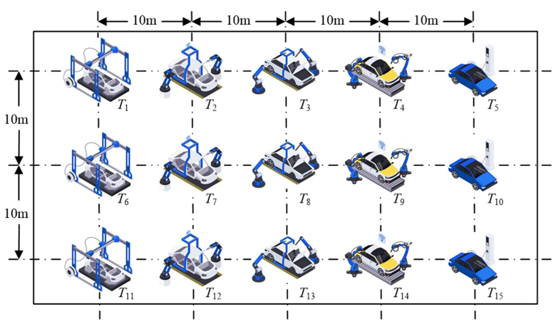
The CMAP can be defined as an undirected assignment graph G   ( T ,   E ) . In the undirected graph, the set of vertices is a task set T = { T 0 ,   T 1 , , T T m a x } , while the set of edges is an assignment set E = { E 01 ,   E 02 , , E n 1 , n } . T 0 indicates the task depot, and each edge E a b = T a , T b E is associated with a travel time k T a , T b t r a v e l from T a to T b . In the aggregation process, different robots gather on the same task to perform different operations, where these different operations occur at different times or locations to avoid collisions when robots aggregate. The set of operations is O = { O T 1 ,   O T 2 , , O T m a x } , and each task T a has a set of operations O T a = { O T a 1 ,   O T a 2 , , O T a m a x } . Hence, each task can be divided into several operations and assigned to a set of robots R = { R 0 ,   R 1 , , R R m a x } for aggregation and implementation. The robots are initially located at task T 0 , and each robot R i has a load ability B R i , which denotes the amount of demand that the robot can reduce per time unit. Additionally, each robot R i has a battery capacity C R i for energy consumption in processing and travel.
A collision-free multi-robot aggregation problem contains four elements C M A P = [ T , O , R , E ] . For a set of solutions X = { x 0 ,   x 1 , , x x m a x } , there is a set of candidate solution x * = { x a b R i } , where the robot selection bit x a b R i = 1 if R i goes from T a to T b and 0 otherwise. In CMAP, the position of each task is fixed, and a swarm of robots can aggregate on a task to complete different operations separately. Different robots do not repeat the same operation. During the aggregation process, collisions between robots also need to be prevented.

4.2. Problem Definition

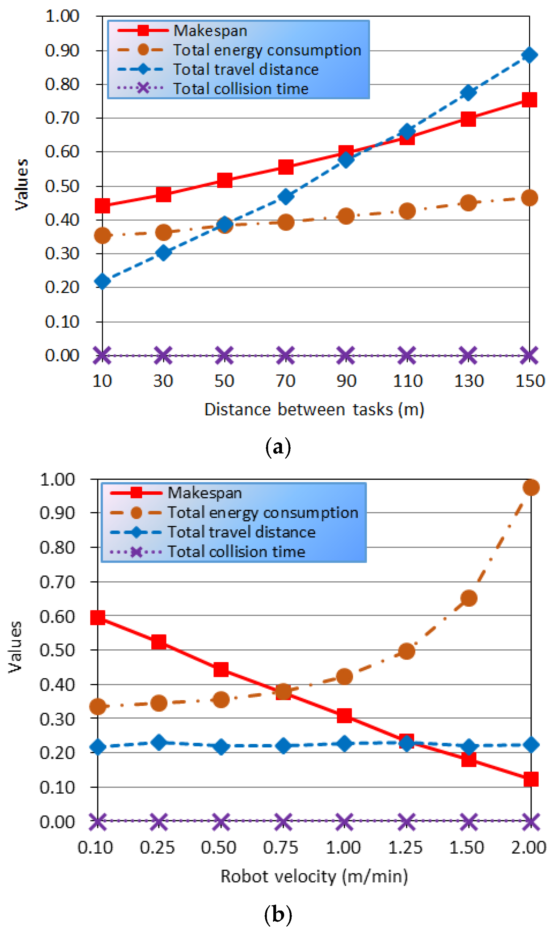
To address the collision-free multi-robot aggregation problem, robots need to be arranged to complete all tasks as soon as possible while, at the same time, ensuring that there is no collision. Therefore, the main objectives include the maximum completion time (makespan) k T m a k e and the collision time k T c o l l of T .
The first objective is the maximum completion time (makespan) k T m a k e of T , which is determined by the difference between the earliest start time k T s t a r t and the latest completion time k T e n d of T , where
k T s t a r t = m i n { k R i , T a s t a r t | T a T , R i R }
k T e n d = m a x { k R i , T a e n d | T a T , R i R }
According to Equations (1) and (2), the maximum completion time (makespan) k T m a k e of T can be obtained as follows:
k T m a k e = k T e n d k T s t a r t
The second objective is the collision time k T c o l l of T , where collision is defined as different robots arriving at the same position at the same time. During the aggregation process, different robots gather on the same task to perform different operations. In order to avoid collisions, different robots handle the same task at different positions or different times. Therefore, the collision time can be calculated based on the time it takes for different aggregation robots to reach and leave the same position when processing the same task, and we have
k T c o l l = T 0 T T m a x | k R i + 1 , O T a j s t a r t k R i , O T a j e n d |
The third objective is the total energy consumption e T t o t a l of T , including the processing energy consumption e T p r o c e of T and the travel energy consumption e T t r a v e l . Considering the processing power p O T a j p r o c e of O T a j , the processing energy consumption e O T a j p r o c e of O T a j can be calculated as follows:
e O T a j p r o c e = p O T a j p r o c e ( k R i , O T a j e n d k R i , O T a j s t a r t ) ; T a [ 1 , T m a x ] ; R i [ 1 , R m a x ] ;
Thus, the processing energy consumption e T a p r o c e of T a can be obtained as follows:
e T a p r o c e = O T a j = 1 O T a m a x e O T a j p r o c e ;   T a [ 1 , T m a x ]
Then, the processing energy consumption e T p r o c e of T can be described as follows:
e T p r o c e = T a T m a x e T a p r o c e ;   T a [ 1 , T m a x ]
Considering the travel power p T a , T b t r a v e l from T a to T b , the travel energy consumption e T a , T b t r a v e l can be calculated as follows:
e T a , T b t r a v e l = p T a , T b t r a v e l ( k R i , T b s t a r t k R i , T a e n d ) ; T a [ 1 , T m a x ] ; R i [ 1 , R m a x ] ;
Then, the travel energy consumption e T t r a v e l of T is
e T t r a v e l = T 0 T m a x e T a , T b t r a v e l ;   T a , T b [ 1 , T m a x ]
According to the processing energy consumption e T p r o c e of T in Equation (7) and the travel energy consumption e T t r a v e l of T in Equation (9), the total energy consumption e T t o t a l of T can be calculated as follows:
e T t o t a l = e T p r o c e + e T t r a v e l
The fourth objective is the total travel distance D T t r a v e l of T , which can be calculated using the travel distance D T a , T b t r a v e l from T a to T b ; that is,
D T t r a v e l = T 0 T m a x D T a , T b t r a v e l ;   T a , T b [ 1 , T m a x ]
Then, the collision-free multi-robot aggregation problem can be described as a four-objective function, considering the maximum completion time (makespan) k T m a k e in Equation (3), the collision time k T c o l l in Equation (4), the total energy consumption e T t o t a l in Equation (10), and the total travel distance D T t r a v e l in Equation (11):
O b j = min ( k T m a k e , min k T c o l l ,   min ( e T t o t a l ) ,   min ( D T t r a v e l ) }
To address the collision-free multi-robot aggregation problem, we need to arrange the aggregation plan of robots to complete all tasks subject to a series of constraints. Whenever a new task is assigned, the robots executing the assigned task form an undirected graph G   ( T ,   E ) . A complex task can be divided into a series of sub-tasks T = { T 0 ,   T 1 , , T T m a x } , enabling each idle robot to aggregate without collision.
As each vertex T a T   is a task, it is associated with three factors: the detection/arrival time k T a ( 0 ) , the inherent increment rate c T a , and the initial demand d T a ( 0 ) . Then, a set of constraints can be obtained.
The first constraint is that a task is unknown by the REI system until it is detected. The emergent demand d T a k of the candidate tasks can be detected by the robotic edge intelligence architecture. The detected demand d T a k of T a accumulated at time k can be obtained as follows:
d T a k = d T a 0 + c T a × ( k k T a 0 ) d T a 0
Each edge E a b = T a , T b E is associated with a travel time k T a , T b t r a v e l from T a to T b . We have
k T a , T b t r a v e l k = k R i , T b e n d k R i , T a s t a r t
where k R i , T b e n d represents the completion time of T b .
The second constraint is that a task cannot be executed before it is detected. Therefore,
k R i , T b s t a r t k T b 0 ; T b [ 1 , T m a x ] ; R i [ 1 , R m a x ]
where k R i , T b s t a r t is the start time of R i at T b .
In particular, the start time k R i , T b s t a r t of R i at T b is determined by the completion time k R i , T a e n d of R i at T a and the travel time k T a , T b t r a v e l from T a to T b ; that is,
k R i , T b s t a r t = a = 0 T m a x   k T a e n d + k T a , T b t r a v e l x a b R i ; T b [ 1 , T m a x ] ; R i [ 1 , R m a x ]
where x a b R i is a robot selection bit ( x a b R i = 1 if R i goes from T a to T b and x a b R i = 0 otherwise). Equation (16) indicates that a robot immediately aggregates to the next task after the completion of the current task.
The third constraint is that a task cannot be executed before the former task is completed; that is,
k R i , T a + 1 s t a r t k R i , T a s t a r t + k R i , T a p r o c e ; T a [ 1 , T m a x ] ; R i [ 1 , R m a x ]
The fourth constraint is that a task cannot be completed before processing is completed; that is,
k R i , T a e n d k R i , T a s t a r t + k R i , T a p r o c e ; T a [ 1 , T m a x ] ; R i [ 1 , R m a x ]
Then, the fifth constraint for the robot selection bit can be described as follows:
x a b R i 0,1 ; a b ; T a , T b [ 1 , T m a x ] ; R i [ 1 , R m a x ]  
The sixth constraint is that the number of incoming paths should equal the number of outgoing paths for each robot at each task; that is,
b = 0 T m a x x a b R i = a = 0 T m a x x b a R i ; T a , T b [ 1 , T m a x ] ; R i [ 1 , R m a x ] ;
where the binary decision variable x b a R i takes a value of 1 if there is a path for R i to go from T b to T a , and 0 otherwise.
The seventh constraint is that each task can be assigned to each robot at most once; that is,
a = 0 T m a x x a b R i 1 ; T a , T b [ 1 , T m a x ] ; R i [ 1 , R m a x ]
The eighth constraint is that the start time and completion time of all the robots at the depot are 0:
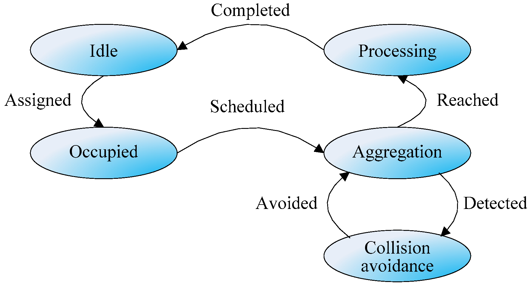
k R i , T a s t a r t 0 = k T a e n d 0 = 0 ; R i [ 1 , R m a x ]
At the final time k R i , T b e n d , all tasks are completed and exit the REI system, and the aggregated robots return to the depot to be reset to an idle state for the next task assignment. It should be noted that all completed tasks should be cleared and all robots should be set as idle again.
The ninth constraint is that the demand for each task must decrease to 0 if it is completed:
d T b ( 0 ) + c T b k T b e n d k T b ( 0 ) = 1 T m a x i = 1 R m a x x a b R i B R i ( k T b e n d k R i , T b s t a r t ) T a , T b [ 1 , T m a x ]
Equation (23) indicates the constraint of load ability B R i . When the task is completed, the accumulated demand at k T b e n d equals the total demand fulfilled by the robots executing until k T b e n d .
The tenth constraint is that the inherent increment rate c T b of T b should be limited in the ability B R i of R i ; that is,
c T b < i = 1 R m a x a = 0 T m a x ( x a b R i B R i ) ; T b [ 1 , T m a x ]
Equation (24) indicates that, for every task, the inherent increment rate of a task must be lower than the total ability of the available robots executing the task, thus ensuring the completion of the task.
The 11th constraint is that the total energy consumption e R i t o t a l of a robot R i should not surpass its battery capacity C R i ; that is,
e R i t o t a l C R i , R i [ 1 , R m a x ]
The total energy consumption e R i t o t a l of R i includes the processing energy consumption e R i p r o c e of R i and the travel energy consumption e R i t r a v e l of R i . According to the robot selection bit x a b R i , which is 1 if R i goes from T a to T b , and 0 otherwise, we have
e R i t o t a l = e R i p r o c e + e R i t r a v e l
e R i p r o c e = O T a j = 1 O T a m a x x a b R i p O T a j p r o c e ( k R i , O T a j e n d k R i , O T a j s t a r t ) ;   T a , T b [ 1 , T m a x ] ; R i [ 1 , R m a x ]
e R i t r a v e l = T a T m a x x a b R i p T a , T b t r a v e l ( k R i , T b s t a r t k R i , T a e n d ) ;   T a , T b [ 1 , T m a x ] ; R i [ 1 , R m a x ]
The objective of the proposed CMAP model is to search for the optimal solution to minimize the objective function in Equation (12) on a set of solutions satisfying Equations (13)–(28).
It is challenging to search for all solutions to the CMAP. Given a solution x = { x 0 ,   x 1 , , x x m a x } and its solution y x for all of the x a b R i values, the makespan can be calculated as follows:
k T m a k e x , y x = m a x T b [ 1 , T m a x ] k R i , T b e n d m i n T a [ 1 , T m a x ] k R i , T a s t a r t
where k R i , T a s t a r t and k R i , T b e n d are calculated from x and y x . In the proposed CMAP model, each code y x is represented as a binary string of robot selection bits for a solution x .
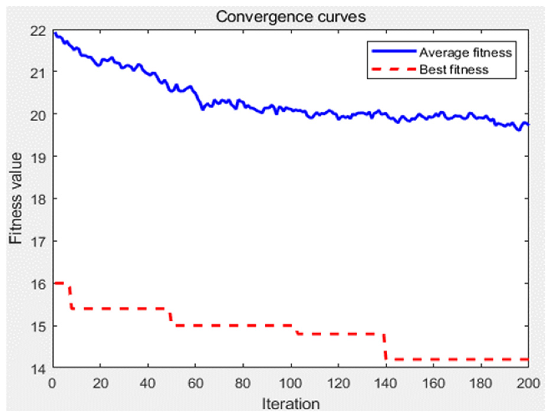
In the aggregation process, the maximum completion time (makespan) k T m a k e and the collision time k T c o l l are evaluated as a value O b j . A task with a shorter processing time, a smaller travel time, and a smaller demand tends to be completed earlier. As the maximum completion time (makespan) k T m a k e and the collision time k T c o l l are often conflicting, and as there are a lot of constraints, it is very difficult to solve the CMAP. In the following section, a novel artificial plant community algorithm is explored in order to help us address the CMAP.

5. An Artificial Plant Community Algorithm

To solve the collision-free multi-robot aggregation problem, this section exploits an artificial plant community algorithm running on a swarm of edge robots. The APC algorithm, proposed in [16,17], is lightweight and has few parameters. It is improved here to enable it to effectively run on the embedded platforms of edge robots and to be suitable under a variable population size. With the edge computing capability of a large number of robots, the improved APC algorithm can help us to search for the optimal solution to the collision-free multi-robot aggregation problem.

5.1. APC-Based REI

The APC algorithm is based on the growth process of a real plant community, which searches for optimal solutions through the heuristic learning of a swarm of plant individuals. For engineering applications, some suggestions for APC-based REI have been proposed, as detailed below.
First, the APC algorithm can be deployed as a local computing method. This refers to running the APC algorithm directly on edge robots or other terminal devices, which enables the data processing and convergence computation of the APC algorithm to be completed locally on the edge robots without the need for network transmission of data. The advantage of this approach is its high efficiency and real-time performance, making it suitable for scenarios with extremely high real-time requirements, such as fire monitoring.
Second, the APC algorithm can also be deployed as an edge computing method. This involves deploying the APC algorithm on edge computing devices in the user’s local area network environment, such as edge boxes or edge routers. The advantages of this approach include fast data processing speed, reduced transmission time of data in the network, and reduced network burden and bandwidth pressure. The APC algorithm uses simple and/or/not operators and is thus suitable for the embedded platforms on edge computing devices.
Third, the APC algorithm can also be deployed as a cloud computing method. In this approach, the APC algorithm is run on the cloud servers for remote access through the Internet, where the cloud servers run the APC algorithm for scheduling and convergence. The associated advantages are strong computing power and ensuring the security and privacy of data. Hence, the APC algorithm may perform better in dynamic aggregation and collision environments, and each edge robot can join or leave the REI system at any time. However, the APC calculation process may result in certain delays and higher costs. If the network is interrupted, the system may not function properly.
Finally, the APC algorithm can also be deployed in a hybrid manner, using a combination of the three methods described above. The advantages of this approach include easy management and expansion, as well as the ability to dynamically adjust the computing resources according to needs; however, it increases the complexity of the APC system. The artificial plant community is randomly distributed on all edge robots or edge servers, and searches for feasible solutions to the collision-free multi-robot aggregation problem.

5.2. Solution Steps of the APC

According to the APC-based REI architecture, the solution steps of the APC algorithm are illustrated in this section in detail. The solution process is composed of five primary steps: initialization, seeding, growing, fruiting, and checking for the end condition. An artificial plant individual can be present in three forms in different solution steps: a seed, an individual, or a fruit. Each artificial plant form can be changed into each other, and the continuous transformation of APC individuals can help us to solve the CMAP.

5.2.1. Initialization

The initialization step includes three sets of parameters: The parameters of the collision-free multi-robot aggregation problem, the APC parameters, and the parameters of the solution system.
The parameters of the collision-free multi-robot aggregation problem include four elements C M A P = [ T , O , R , E ] , including a task set T = { T 0 , T 1 , , T T m a x } , the operation set O = { O T 1 , O T 2 , , O T m a x } , a set of robots R = { R 0 , R 1 , , R R m a x } , and the assignment edge set E = { E 01 , E 02 , , E n 1 , n } . Each task T a has a set of operations O T a = { O T a 1 , O T a 2 , , O T a m a x } . The robots are initially located at task T 0 , and each robot R i has a load ability B R i and a battery capacity C R i .
The APC parameters include the population size S , the selection bits of a robot set { x a b R i } , the seeding probability p s e e d , the growing probability p g r o w , and the fruiting probability p f r u i t . Hence, as a candidate solution set, X = { x 1 , x 2 , , x s , , x S } represents an artificial plant community, where x s ={ x a b R i } . The objective function O b j in Equation (12) can be introduced as a fitness function for the APC algorithm:
f i t = C o n s t O b j
where C o n s t is a sufficiently large positive constant. Here, the higher the fitness f i t is, the better the artificial plant individuals. The fitness function f i t in Equation (30) can help the APC algorithm to choose the best individuals.
The parameters of the solution system are composed of the error threshold e t h and the maximum number of iterations I t e m a x , where the iteration counter I t e is initially set to be zero.

5.2.2. Seeding of the APC

The seeding process endows the APC with a global search capability, where all APC individuals are in the form of seeds randomly generated in the whole candidate solution space. The random search capability can help to search for more candidate solutions to the collision-free multi-robot aggregation problem, which is defined by a seeding probability p s e e d . There are two scenarios to produce the seeds in the seeding stages.
The first seeding scenario is in the first iteration after initialization. There are no individuals or fruits generated in previous iterations, and initial seeds with a population size S will be randomly generated in the edge robots.
The second seeding scenario occurs in the following iterations. Therefore, fruits generated in the previous fruiting steps with a population size of S can be selected as a part of the seeds, and another part of random seeds with a population size of p s e e d × S is also produced. These two types of seeds contain elites and random solutions and have a greater population size of ( 1 + p s e e d ) × S .
An artificial plant seed x s can be encoded as a binary string for robot assignment, as shown in Equation (31):
x s = { x a b R i }
A binary bit x s = 1 indicates that a task edge E a b = T a , T b E from tasks T a to T b is selected as the candidate solution of robot R i , while x s = 0 represents that a task edge E a b = T a , T b E is not chosen as the candidate solution.
Therefore, the lower the seeding probability p s e e d , the weaker the global search ability, but the faster the convergence rate, possibly even resulting in premature convergence to a local optimum, and vice versa.

5.2.3. Growth of the APC

The survived seeds are determined by the growing probability p g r o w and a fitness function. The artificial plant seeds with high fitness can grow to generate more fruits, while the other seeds with low fitness do not survive and are removed. Hence, the population size of the APC in the growing stage is reduced to a small value of p g r o w × S , with the size of the removed population being (1 − p g r o w ) × S . On some edge robots with population size (1 − p g r o w ) × S , there may be no artificial plant individual; however, other edge robots with a population size p g r o w × S may contain elite individuals. Based on the fitness function f i t in Equation (30), the growing individuals x s * can be calculated as follows:
x s * = { x s * | f i t x s * S p g r o w f i t ( x s S ( 1 p g r o w ) ) }
To choose the best candidate solution in the growing operation, various sorting methods can be employed, such as the direct sort, bubble sort, merge sort, select sort, quick sort, and so on. Different sorting algorithms may have different advantages in terms of temporal and spatial performance. Now, the plant individual with the highest fitness can be selected as the optimal solution. Based on the growing individuals x s * selected using Equation (32), the best candidate solution can be defined as x s # in Equation (33):
x s # ( t ) = { x s # | f i t x s # = m a x [ f i t x s * ] }
The local search ability of the APC is determined by the growing probability p g r o w . The lower the growing probability p g r o w , the higher the convergence rate, but the lower the global search ability; as such, a low growing probability p g r o w may result in a premature convergence to local optima and vice versa.

5.2.4. Fruiting of the APC

The fruiting operation endows the APC with a social learning capability, where the elite plant individuals with high fitness can learn from each other to generate more offspring fruits. This social learning process allows the swarm intelligence of edge robots to search for more candidate solutions, such that the population size increases to its original value S .
For the best individual x s # with the highest fitness, the fruiting operation will generate identical offspring to preserve the elite information, as shown in Equation (34):
x s ( k + 1 ) = x s # ( k )
For all individuals, social learning occurs between different individuals to generate more feasible solutions, with a population size of S 1 .
A cross-factor C f r u i t can help us decide how many parents exchange information each time to produce offspring. If C f r u i t = 1 , parthenogenesis is considered and it is suitable to preserve the best candidate solution (i.e., there is no social learning, only self-learning).
If C f r u i t = 2 , two individuals are employed to generate an offspring each time, and each offspring is composed of social learning information from two parents. If it is assumed that there are two parents x s ( k 1 ) = { x s 1 ( k 1 ) , , x s l ( k 1 ) , x s l + 1 ( k 1 ) , } and x s ( k 1 ) = { x s 1 ( k 1 ) , , x s l ( k 1 ) , x s l + 1 ( k 1 ) , } , a fruit with C f r u i t = 2 is shown in Equation (35):
x s ( k ) = { x s 1 ( k 1 ) , x s 2 ( k 1 ) , , x s l ( k 1 ) , x s l + 1 ( k 1 ) , k Or   x s ( k ) = { x s 1 ( k 1 ) , x s 2 ( k 1 ) , , x s l ( k 1 ) , x s l + 1 ( k 1 ) , }
If C f r u i t 3 , three or more individuals are employed to learn from each other, but it also makes the calculation process more complex. Assuming the three parents x s ( k 1 ) = { , x s l k 1 , } , x s ( k 1 ) = { , x s l k 1 , } , and x s ( k 1 ) = { , x s l k 1 , } , a possible offspring is shown in Equation (36).
x s ( k ) = { x s 1 k 1 , , x s l k 1 , , x s ( l + 1 ) ( k 1 ) , }
In particular, the social learning process helps the APC to recover the population size to the initial value S .
In summary, a higher p f r u i t can retain more information about elites and accelerate the convergence performance. On the contrary, a lower p f r u i t makes it easier to destroy the information obtained from elites, making it less likely to converge to local optima early.

5.2.5. Checking for the End Condition

The robotic edge devices search for the optimal candidate solutions to the collision-free multi-robot aggregation problem through iterative edge computing of the artificial plant community algorithm. Therefore, a series of end conditions should be preset to instruct the edge robots to justify whether the iteration will be stopped before the optimal candidate solution is output to assign the robots to various tasks and avoid collisions.
The best candidate solution x s # ( t ) at time t has the fitness f i t [ x s # t ] according to Equation (33), and the best candidate solution x s # ( k 1 ) at the previous time step ( k 1 ) has fitness f i t [ x s # k 1 ] . Hence, the error between two adjacent moments k and ( k 1 ) can be calculated as follows:
e r r o r ( k ) = | f i t x s # k f i t [ x s # k 1 ] |
Then, an error threshold e t h can be introduced to determine whether the iterative calculation process can be completed.
i f   e r r o r ( k ) e t h , t h e n   g o   t o   e n d . e l s e ,   t h e n   r e t u r n   t o   t h e   s e e d i n g   s t e p .
If the edge robots determine that the e r r o r ( k ) in Equation (36) is not higher than the predefined threshold e t h , then the iteration can be completed, and the optimal candidate solution x s # t can be output for assignment. Otherwise, the fruits obtained from this calculation will serve as the seeds for the next iteration, starting a new round of iteration until the end conditions are met.

5.3. Algorithm Flow

As shown the APC algorithm flow shown in Figure 4, based on the iterative execution of the seeding, growing, and fruiting operations, the edge robots can search for the optimal candidate solution to the collision-free multi-robot aggregation problem through the swarm intelligence of multi-robot systems.
The algorithm flow in Figure 4 is composed of five primary steps and a big loop, including initialization, seeding operation, growing operation, the fruiting operation, and checking for the end condition. During initialization, the parameters of CMAP, the APC parameters, and the solution system parameters—that is, the fitness function in Equation (30)—are defined. In the seeding operation, random seeds are generated according to the seeding probability pseed, and seeds are produced from the previous fruits. In the growing operation, fitness calculation and comparison are conducted in order to determine the optimal seeds to grow according to the growing probability pgrow, selecting the seeds with the highest fitness. In the fruiting operation, fruits are generated according to the fruiting probability pfruit, and optimal fruits are generated via parthenogenesis. After checking for the end condition, the APC will decide to continue the calculation loop or output the optimal candidate solution to the CMAP.
According to the APC algorithm flowchart shown in Figure 4, the pseudo-code for robotic edge implementation is shown in Algorithm 1. This algorithm describes the solution process of the APC algorithm with respect to the collision-free multi-robot aggregation problem, where the candidate solution is encoded using Equation (31), the fitness function is that given in Equation (30), and the constraints are Equations (13)–(28). The task state transition process is shown in Figure 2, and the robot state transition process is shown in Figure 3.
Algorithm 1: The APC to solve the CMAP
Applsci 15 04240 i001
Then, the best candidate solution to the CMAP will be output for robot assignment. Algorithm 1 depicts the solution process for a collision-free multi-robot aggregation problem, where the APC individuals are encoded as a feasible solution via Equation (31). The fitness function in Equation (30) and constraints in Equations (13)–(28) are employed to instruct the APC to search for the optimal candidate solutions. When implementing the optimal candidate solution, the robots will be assigned to a suitable task, and the state transitions of tasks and robots will change during assignment. In Algorithm 1, after a task is completed, the completed task disappears from the REI system and will no longer be reused, while the robot that completed the task can be reused for the next task. Overall, when the number of robots is N, the computational complexity of this algorithm is O ( N 2 ) .

6. Benchmark Data and Experiments

This section describes the design of a series of benchmark data used to test the proposed REI-based method in order to solve the collision-free multi-robot aggregation problem, including the benchmark data set, experimental results, and performance comparison.

6.1. Benchmark Test Set

To test the collision-free multi-robot aggregation problem solution process, the benchmark data used in [18,19] are introduced and modified herein, which were collected in a production workshop scenario. Based on the proposed REI model, the benchmark data were modified to reflect a scenario with 15 fixed tasks, 15 operations, and 15 robots, which is more complex than the benchmark tests detailed in [18,19]. In [18], 15 flowing jobs and 15 fixed machines were considered but not transportation; meanwhile, in [19], 15 flowing jobs, 8 fixed machines, and 15 AGVs were considered. Due to the more complex obstacle placements and higher robot densities, we designed a unidirectional loop consisting of 15 fixed tasks with a total length of 140 m and an equal distance between consecutive tasks of 10 m, as shown in Figure 5. Based on the layout of the actual production systems used in [18,19], Figure 5 provides the benchmark test roadmap of the 15 fixed tasks to simplify the calculations and as a benchmark comparison for international peers.
In Figure 5, there is a 10 m interval between adjacent pairs of the 15 fixed tasks T = { T 1 , T 2 , , T 15 }, where the considered distance is the Manhattan distance between tasks. For example, the travel distance D 1,8 between T 1   a n d   T 8 can be obtained as 30 m. Hence, the travel distances [ D i j ] between consecutive tasks can be represented as follows (in m):
[ D i j ] = 10 20 10 10 20 10 30 40 10 20 30 20 10 20 30 20 30 40 10 20 30 20 10 20 50 20 30 40 30 20 30 40 30 40 50 60 30 40 50 20 30 40 30 20 10 40 30 20 10 20 30 10 40 10 50 40 50 30 20 10 40 30 20 10 20 30 20 50 40 10 60 50 40 10 20 30 20 30 40 30 20 30 40 50 20 10 20 30 20 10 40 30 20 50 40 30 20 30 40 30 20 30 40 30 40 50 40 30 60 50 40 30 40 10 20 30 20 10 20 30 20 10 40 50 60 10 40 50 20 60 80 60 20 30 40 30 20 50 10 20 10 10 20 10 30 20 10 20 30 40 10 20 30 40 20 40 30 20 10 40 30 20 30 20 10 20 30 20 10 40 30 50 40 50 10 40 10 60 40 20 20 30 20 10 40 30 20 30 40 10 20 30 20 10 20 30 20 10 20 30 40 10 20 30 10 20 10 10 20 10
Our modified benchmark test has an entrance at task 1, where 15 robots are allowed to be in task 1 initially and can enter or exit the task at any time. The robot speed is limited to between 0.2 m/s and 2 m/s, divided into five different speed levels.
Table 3 shows the processing times k O T a j p r o c e for the 15 tasks T = T 1 , T 2 , , T 15 , about twice the number of machines in [19]. This modification is more suitable for our complex multi-robot system and the benchmark data are consistent with real-world cases [18]. Comparing with the travel distances in [ D i j ] and the average speed of the robots of about 0.5 m/s, the processing times in Table 3 are greater. As adjusted data referring to the existing literature [18,19] were developed to meet the requirements of multi-robot systems and serve as a proxy to a real-world multi-robot aggregation problem, this adjustment was considered more suitable for our benchmark tests with robot travel.
Table 4 lists the processing power p O T a j p r o c e for each task, which was modified from the setup power in [19]. Hence, the processing energy consumption e T a p r o c e and e O T a j p r o c e can be obtained by the product of the processing power values and the processing times in Equations (6) and (7).
The travel power p T a , T b t r a v e l of the robots with different speed rates is shown in Table 5 after modifying the travel power in the benchmark test data [19]. The energy consumption can be obtained by multiplying the travel power values by the travel times using Equations (8) and (9). Compared with the benchmark data [19], there was no apparent modification in the average robot power, as robots only need to walk during the aggregation process, without the need to move goods or transport. Therefore, a robot was considered to consume 0.90–1.22 kW of energy for each operation of a task and 82.8 W to travel at a speed of 0.5 m/s.
Some assumptions were made to simplify the experimental analysis, as follows:
Assumption 1.
It is assumed that the battery carried by the robot has sufficient capacity; there is no need to consider the charging caused by insufficient battery capacity. As the battery of a robot is sufficient to finish multiple tasks after being fully charged, it is reasonable not to consider additional charging during the execution of each task.
Assumption 2.
It is assumed that there is no difference between robots, machines, tasks, or cargo, and human interference, environmental disturbances, malfunctions, and accidents are not considered.
Assumption 3.
It is assumed that different tasks are independent, and different robots are also independent. The intrinsic connections between different tasks are not considered, nor the connections between different robots.
Assumption 4.
It is assumed that different robots perform the same operation without considering any differences in operational details, including different robot walking methods, different manipulating arms, and different levels of power consumption caused by various operations.

6.2. Benchmark Test Results

This section provides the benchmark test results for the proposed APC algorithm. The multi-objective function in Equation (30) is employed for natural selection, which includes the maximum completion time (makespan) k T m a k e in Equation (3), the collision time k T c o l l in Equation (4), the total energy consumption e T t o t a l in Equation (10), and the total travel distance D T t r a v e l in Equation (11). The fitness function is Equation (30). The APC simulation parameters include the population size = 80, the seeding probability p s e e d = 0.2 , the growing probability p g r o w = 0.7 , the fruiting possibility p f r u i t = 0.1 , and the cross-factor C f r u i t = 2 .
The end conditions included the maximum number of iterations I t e m a x = 200 and the maximum computation time = 1.0 h. The simulation system was characterized by an AMD Ryzen 3 4300U with Radeon Graphics 2.70 GHz CPU, 8.00 GB RAM, 64-bit Windows 10 operating system, and the MATLAB R2018a simulation software.
Figure 6 presents the processing time for the collision-free multi-robot aggregation problem. The horizontal axis gives the processing time, the vertical axis shows the number of tasks, and the right side presents the travel time, processing time, and makespan of each robot (in fractional form). Each progress bar in Figure 6 is labeled with three numbers enclosed in parentheses, denoting the task number T a , operation number O T a j , and processing time k O T a j p r o c e . The Gantt chart shows the robot aggregation results and processing time under the minimum makespan, with different tasks marked with different colors. The makespan value in Figure 6 is k T m a k e = 14.0280 h, and the processing power consumption can be calculated to be e T p r o c e = 123.404 kWh, according to the corresponding processing time. Although the travel time value is given on the right, it is not visible in the graph.
Figure 7 shows the travel time for collision-free multi-robot aggregation. The horizontal axis shows the travel time, the vertical axis lists the number of robots, and the right side indicates the travel time and makespan of each robot (in fractional form). All progress bars in Figure 7 are labeled with three numbers enclosed in parentheses, including the task number, operation number, and travel time. Figure 7 verifies the robot aggregation results and travel Gantt chart in accordance with the makespan shown in Figure 6. The total collision time was k T c o l l = 0.0 h and, so, the proposed scheduling method realized the collision-free objective. The makespan of the travel time in Figure 7 is k T a , T b t r a v e l = 13.9280 h, and the corresponding travel energy consumption of T can be obtained as e T t r a v e l = 0.2670 kWh. Therefore, the total energy consumption of all tasks was calculated as e T t o t a l = 123.6710 kWh. The maximum travel distance in Figure 7 is m a x D T a , T b t r a v e l = 440 m, and the minimum travel distance is m i n D T a , T b t r a v e l = 300 m, while the total travel distance D T t r a v e l is 5800 m.
After 300 tests, the statistics of the benchmark test are summarized in Table 6, where the results demonstrate that the proposed APC algorithm can help us to search for the optimal solution to the collision-free multi-robot aggregation problem. It can be seen that the minimum value of makespan k T m a k e presented an increase of about 14.55% compared to the maximum value, the total travel distance D T t r a v e l (m) had an increase of about 6.90% compared to the maximum value, and the minimum value of travel energy consumption e T t r a v e l had an increase of 6.90% compared to the maximum value. There is a positive correlation between the total robot energy consumption (kWh) and the maximum travel distance (m) and the travel speed (m/s) in Table 5, where the total processing energy (kWh) of robots was 430.33–462.24 times greater than the travel energy consumption (kWh). The statistical data indicate the total collision time k T c o l l = 0.0 h, verifying that the collision-free objective was satisfied in the multi-robot aggregation problem.
Figure 8 shows the convergence curves of the proposed APC algorithm, including the average fitness of the APC population and the best fitness of the optimal solution. The benchmark test results in Figure 6 and Figure 7 were calculated with a maximum number of iterations equal to 200. It can be observed, from Figure 8, that the optimal solution can be obtained by the proposed APC algorithm after about 140 iterations, showing the good convergence performance of the proposed APC algorithm in solving the collision-free multi-robot aggregation problem.
To delve deeper into the entangled factors affecting the collision-free multi-robot aggregation problem, the benchmark results under changing parameters are shown in Figure 9a,b, describing how variations in the parameters affected the main metrics (i.e., the makespan k T m a k e , total collision time k T c o l l , total travel distance D T t r a v e l , and total energy consumption e T t o t a l ). To present the different variation curves in the same graph, all data were normalized.
The trends of the four main metrics with different distances between tasks are shown in Figure 9a. It can be observed that the the collision-free goal of k T c o l l = 0.0 h is reached, where a greater distance between tasks increased the makespan k T m a k e , total travel distance D T t r a v e l , and the total energy consumption e T t o t a l . When the distance between tasks was in the range of 90–150 m, the makespan k T m a k e rapidly increased. Maintaining the distance between tasks in the range of 50–90 m is helpful to balance the makespan k T m a k e and the energy consumption e T t o t a l , as the total travel distance D T t r a v e l will decrease and less time will be consumed for aggregation.
The trends of the four main metrics under different robot velocities are shown in Figure 9b. It can be seen that a greater robot velocity is helpful to decreasing the makespan k T m a k e when the collision-free goal of k T c o l l = 0.0 h is achieved. However, a greater robot velocity will increase the total energy consumption e T t o t a l , while the total travel distance D T t r a v e l remains stable. When the robot velocity is in the range of 1.0–2.0 m/s, the total energy consumption e T t o t a l will rapidly increase. Therefore, maintaining the robot velocity in the range of 0.5–1.0 m/s helps to balance the makespan k T m a k e and the energy consumption e T t o t a l , as less time will be consumed for robot aggregation and collision avoidance.
Considering Figure 6, Figure 7, Figure 8 and Figure 9, the travel energy consumption is less than the processing energy consumption, and more robots are helpful to improving task efficiency while maintaining a low makespan k T m a k e . To the contrary, fewer robots will tend to increase the makespan k T m a k e and reduce task efficiency. Additionally, the energy conservation effect caused by fewer robots is less than the increase in the makespan value k T m a k e . For engineering applications, performing tasks at an economical speed helps to conserve energy, and more robots and more energy consumption at faster aggregation velocity can help to improve task efficiency.

6.3. Performance Comparison

Some state-of-the-art algorithms were employed for comparison, including the proposed APC algorithm, grey wolf optimization (GWO) [2], the genetic algorithm (GA) [3], particle swarm optimization (PSO) [4], ant colony optimization (ACO) [7], and deep learning (DL) [8].
All of these SOTA algorithms adopted the same benchmark data described in Section 6.1 and the multi-objective function in Equation (12). Each technique uses a basic version and the same population size. The APC algorithm used the same parameters as detailed above. For GWO, the population size of the gray wolves was set to S = 80, the upper bound of the variables was set as ub = [10, 10], the lower bound of variables was set as lb = [−10, −10], and the dimension of the problem was set as dim = 2. For the GA, the population size was S = 80, the chromosome length was Lind = 20, the crossover probability was px = 0.7, and the mutation probability was pm = 0.01. For the PSO, the population size was set as S = 80, the location limitation was 0.5, the speed limitation was [−0.5, 0.5], the self-learning factor was c1 = 1.5, and the social learning factor was c2 = 1.5. The ACO parameters were set as follows: pheromone importance = 1.0, importance of heuristic factors = 5.0, pheromone volatilization factor = 0.1, and S = 80 ants. For the DL models, a convolutional neural network with six convolution cores, six input channels (cin = 6), and six output channels (cout = 6) was used. The learning rate of the offset item was twice that of the weight. The extension edge was set to 0, the weight was initialized to Gaussian, and the value of the constant offset item was 0.
Two scenarios were employed for comparison, i.e., different task numbers and different robot numbers, as detailed in Table 7 and Table 8. The number of tasks was increased from T m a x = 1,3 , 5 , to T m a x = 15 , and the number of robots was increased from R m a x = 1,3 , 5 , to R m a x = 15 . All algorithms run with the same number of iterations and the same computation time. For all algorithms, the maximum number of iterations was set to I t e m a x = 200 , and the maximum computation time was 1.0 h. Five main metrics were used for the benchmark comparison: the makespan k T m a k e , total collision time k T c o l l , total energy consumption e T t o t a l , total travel distance D T t r a v e l , and the solution time. As these metrics are differently scaled, the results of all metrics were normalized into the range from 0 to 1. The solution time is provided in seconds. Note that the optimal results in Table 7 and Table 8 are highlighted in bold.
Table 7 shows the comparison results of benchmark tests using the six heuristic algorithms with different numbers of tasks. The first line of Table 7 presents the total number of tasks, with nine scenarios in total, including the mean value. The first column lists the APC, GWO, GA, PSO, ACO, and DL. It can be observed that more tasks tended to increase the makespan for all algorithms, as well as the energy consumption. Table 7 indicates that the makespan k T m a k e , total energy consumption e T t o t a l , and total travel distance D T t r a v e l improved differently with the algorithms used. In summary, the proposed APC algorithm could more easily obtain better mean values for makespan and energy consumption, as highlighted in bold in the table. Compared with the other SOTA algorithms, the proposed APC algorithm improved the makespan k T m a k e by up to 3.09%, total energy consumption e T t o t a l by up to 3.38%, and total travel distance D T t r a v e l by up to 3.42% while maintaining no collisions ( k T c o l l = 0).
Table 8 presents a comparison of the results obtained using the six heuristic algorithms with different numbers of robots, where the first line of Table 8 lists the considered number of robots. The first column lists the APC, GWO, GA, PSO, ACO, and DL algorithms, where each adopted the same parameters as above. The comparative results in Table 8 indicate that the metrics were optimized by the different algorithms to various degrees, whereby the proposed APC algorithm obtained the best mean values for each metric (highlighted in bold). For the main metrics, the proposed APC algorithm improved the makespan k T m a k e by up to 3.06%, total energy consumption e T t o t a l by up to 3.15%, and total travel distance D T t r a v e l by up to 2.68% while maintaining no collisions ( k T c o l l = 0). Regarding solution speed, the APC had a great advantage over the DL model, as the latter required more computational time to search for comparable solutions. In summary, under a varying number of robots, the APC algorithm can search for the optimal solutions with fast convergence while effectively avoiding local optima.
According to the performance comparison in Table 7 and Table 8, the most efficient algorithm was the APCbefore DL and GA. To achieve an optimal makespan without collision, robots must be assigned to aggregate on different tasks and complete operations as soon as possible. Considering the collision-free multi-robot aggregation problem, the proposed APC algorithm demonstrated clear advantages in searching for optimal solutions over the other SOTA algorithms.

6.4. Discussion

First, in our benchmark experiment, 15 robots were employed to implement the edge computing architecture detailed in Section 3. The success of the experiment also proved the feasibility of the proposed edge intelligence approach. When the number of robots increases, the APC algorithm can even improve edge computing capabilities.
Second, our benchmark experiment used the objective function and constraints established in Section 4, including the maximum completion time (makespan) k T m a k e , the collision time k T c o l l , the total energy consumption e T t o t a l , and the total travel distance D T t r a v e l . The experimental results indicate that the established problem model effectively describes the CMAP.
Third, from Figure 6, Figure 7, Figure 8 and Figure 9 and Table 6 in Section 6.2, as well as Table 7 and Table 8 in Section 6.3, it can be seen that simple parameters and fast calculation ability make the APC algorithm very suitable for deployment on robotic edge computing platforms. Compared with other heuristic optimization methods, including ACO, GA, PSO, or standard APC, the improved APC algorithm uses random seeding in each iteration to increase its global search capability and enhance its local convergence ability through an increased probability of crossing growing individuals. When the number of robots is N, the computational complexity of this algorithm is O ( N 2 ) . The same parameters were used to develop the SOTA methods used for comparison; however, this does not mean that the algorithms will perform similarly under the same conditions, as each has specific functioning characteristics.
Fourth, our benchmark test data took into account the collision problem during multi-robot aggregation, and all data have been accurately presented in the manuscript (i.e., Figure 5, Table 3, Table 4 and Table 5 in Section 6.1). Therefore, international peers can reproduce the data themselves and conduct further research.
Fifth, the experimental results presented in this section also demonstrated that the combination of robotic edge computing platforms and artificial intelligence in engineering applications is feasible and promising. The developed robotic edge intelligence approach can be expected to help in solving many engineering problems in the context of industrial automation, autonomous transportation, and search-and-rescue operations without the need to upgrade expensive hardware and software.
Finally, there are some differences between running algorithm on systems with edge computing and without edge computing. In an edge computing system, the response time of algorithms is significantly reduced, making such a system especially suitable for latency-sensitive applications, such as real-time autonomous driving, industrial automation, and so on. In a system without edge computing, algorithms are easily affected by single points of failure and may have difficulty in performing large-scale data processing.

7. Conclusions

This study first attempted to survey the collision-free multi-robot aggregation problem and, consequently, developed a novel robotic edge intelligence model to address the CMAP. Our work includes four main contributions, as follows: First, four metrics of the collision-free multi-robot aggregation problem were considered, including the minimum makespan, collision avoidance, energy consumption, and total travel distance. Second, a novel heuristic algorithm is designed to search for the optimal solution, namely, the artificial plant community algorithm. Third, a newly developed benchmark test set based on the existing literature was explored. The experimental results demonstrated that the proposed APC algorithm presents improved global and local search capabilities, and is superior to some state-of-the-art methods in solving the CMAP. Regarding the efficiency of task execution, the proposed APC algorithm improved makespan k T m a k e by up to 3.06%, the total energy consumption e T t o t a l by up to 3.15%, and the total travel distance D T t r a v e l by up to 2.68%, while maintaining no collisions ( k T c o l l = 0). At the same time, the proposed APC method is lightweight; as such, it can be easily deployed on the embedded platforms of edge robots. The performance comparison demonstrated that the APC algorithm can efficiently instruct the edge robots to aggregate and handle tasks without collision.
However, there are still some shortcomings that need to be further resolved. First, while this work built a multi-objective function for the CMAP, it was based on a certain environment and assumptions. For engineering applications, it is required to consider more factors and uncertain environments to ensure collision avoidance. Second, our edge intelligence approach was not deployed in real-world scenarios and, in future research, how to deploy and validate edge intelligence in real-world scenarios is an important direction. This work investigated some main metrics, but other metrics were not considered—such as the collision rate, path efficiency, convergence time, and resource utilization—which should be further surveyed in the future. Third, there may be differences between running the proposed algorithm in systems characterized by edge computing and those without edge computing, potentially leading to hardware limitations, communication delays, sensor inaccuracies, and environmental uncertainties, which are not considered in this manuscript. In the future, it will be necessary to further study the developed mathematical model and working processes, as well as conducting further comparative experiments. Finally, even though the proposed APC can efficiently handle the collision-free multi-robot aggregation problem, it will be important to test and analyze the impacts of environment size, obstacle density, and computational resources on performance in the future, using more real-world benchmark data and statistical tools.

Author Contributions

Conceptualization, Z.C.; Methodology, Z.C.; Software, Z.L. (Zhuimeng Lu); Validation, Z.L. (Zhuimeng Lu) and Z.L. (Zeya Liu); Investigation, Z.L. (Zhuimeng Lu); Data curation, Q.Y. and Z.L. (Zeya Liu); Writing – original draft, Q.Y.; Writing – review & editing, Q.Y.; Project administration, Z.C. and G.G.; Funding acquisition, Z.C. and G.G. All authors have read and agreed to the published version of the manuscript.

Funding

This work was supported in part by the National Natural Science Foundation of China (No. 71471102), Major Science and Technology Projects in Hubei Province of China (Grant No. 2020AEA012), and Yichang University Applied Basic Research Project in China (Grant No. A17-302-a13).

Institutional Review Board Statement

Not applicable.

Informed Consent Statement

Not applicable.

Data Availability Statement

The original contributions presented in the study are included in the article, further inquiries can be directed to the corresponding author.

Conflicts of Interest

The authors declare no conflict of interest.

Abbreviations

AbbreviationsFull forms
ABCArtificial bee colony
ACOAnt colony optimization
APCArtificial plant community
AGVAuto-guided vehicle
CMAPCollision-free multi-robot aggregation problem
DLDeep learning
ERLEdge robot layer
ESLEdge server layer
FLFuzzy logic
GAGenetic algorithm
GWOGrey wolf optimization
JSPJob–shop scheduling problem
PSOParticle swarm optimization
RLReinforcement learning
REIRobotic edge intelligence
UAVUnmanned aerial vehicle
USVUnmanned surface vehicle
WOAWhale optimization algorithm

References

  1. Hao, Z.; Mayya, S.; Notomista, G.; Hutchinson, S.; Egerstedt, M.; Ansari, A. Controlling collision-induced aggregations in a swarm of micro bristle robots. IEEE Trans. Robot. 2023, 39, 590–604. [Google Scholar] [CrossRef]
  2. Tang, H.W.; Sun, W.; Lin, A.P.; Xue, M.; Zhang, X. A GWO-based multi-robot cooperation method for target searching in unknown environments. Expert Syst. Appl. 2021, 186, 115795. [Google Scholar] [CrossRef]
  3. Gao, G.; Mei, Y.; Xin, B.; Jia, Y.-H.; Browne, W.N. Automated coordination strategy design using genetic programming for dynamic multipoint dynamic aggregation. IEEE Trans. Cybern. 2021, 52, 13521–13535. [Google Scholar] [CrossRef]
  4. Liu, X.F.; Fang, Y.C.; Zhan, Z.H.; Zhang, J. Strength learning particle swarm optimization for multiobjective multirobot task scheduling. IEEE Trans. Syst. Man Cybern.-Syst. 2023, 53, 4052–4063. [Google Scholar] [CrossRef]
  5. Misir, O.; Gökrem, L.; Can, M.S. Fuzzy-based self organizing aggregation method for swarm robots. Biosystems 2020, 196, 104187. [Google Scholar] [CrossRef]
  6. Wu, W.; Tong, S.C. Collision-free adaptive fuzzy formation control for stochastic nonlinear multiagent systems. IEEE Trans. Syst. Man Cybern.-Syst. 2023, 53, 5454–5465. [Google Scholar] [CrossRef]
  7. Gao, G.; Mei, Y.; Jia, Y.-H.; Browne, W.N.; Xin, B. Adaptive coordination ant colony optimization for multipoint dynamic aggregation. IEEE Trans. Cybern. 2021, 52, 7362–7376. [Google Scholar] [CrossRef]
  8. Le, H.C.; Saeedvand SHsu, C.C. A comprehensive review of mobile robot navigation using deep reinforcement learning algorithms in crowded environments. J. Intell. Robot. Syst. 2024, 110, 158. [Google Scholar] [CrossRef]
  9. Sadeghi Amjadi, A.; Bilaloğlu, C.; Turgut, A.E.; Na, S.; Şahin, E.; Krajník, T.; Arvin, F. Reinforcement learning-based aggregation for robot swarms. Adapt. Behav. 2023, 32, 265–281. [Google Scholar] [CrossRef]
  10. Deng, S.G.; Zhao, H.L.; Fang, W.J.; Yin, J.W.; Dustdar, S.; Zomaya, A.Y. Edge intelligence: The confluence of edge computing and artificial intelligence. IEEE Internet Things J. 2020, 7, 7457–7469. [Google Scholar] [CrossRef]
  11. Haddadin, S.; De Luca, A.; Albu-Schäffer, A. Robot collisions: A survey on detection, isolation, and identification. IEEE Trans. Robot. 2017, 33, 1292–1312. [Google Scholar] [CrossRef]
  12. Qin, X.; Yang, Y.; Pan, M.; Cui, L.; Liu, L. Morphobot: A platform for morphogenesis in robot swarm. IEEE Robot. Autom. Lett. 2023, 8, 7440–7447. [Google Scholar] [CrossRef]
  13. Garg, V. E2RGWO: Exploration enhanced robotic GWO for cooperative multiple target search for robotic swarms. Arab. J. Sci. Eng. 2022, 48, 9887–9903. [Google Scholar] [CrossRef]
  14. Misir, O.; Gökrem, L. Dynamic interactive self organizing aggregation method in swarm robots. Biosystems 2021, 207, 104451. [Google Scholar] [CrossRef]
  15. Misir, O.; Gökrem, L. Flocking-based self-organized aggregation behavior method for swarm robotics. Iran. J. Sci. Technol.-Trans. Electr. Eng. 2021, 45, 1427–1444. [Google Scholar] [CrossRef]
  16. Cai, Z.; Ma, Z.; Zuo, Z.; Xiang, Y.; Wang, M. An image edge detection algorithm based on an artificial plant community. Appl. Sci. 2023, 13, 4159. [Google Scholar] [CrossRef]
  17. Cai, Z.; Du, J.; Huang, T.; Lu, Z.; Liu, Z.; Gong, G. Energy-efficient collision-free machine/AGV scheduling using vehicle edge intelligence. Sensors 2024, 24, 8044. [Google Scholar] [CrossRef]
  18. Gu, X. Application research for multiobjective low-carbon flexible job-shop scheduling problem based on hybrid artificial bee colony algorithm. IEEE Access 2021, 9, 135899–135914. [Google Scholar] [CrossRef]
  19. Boufellouh, R.; Belkaid, F. Multi-objective optimization for energy-efficient flow shop scheduling problem with blocking and collision-free transportation constraints. Appl. Soft Comput. 2023, 148, 110884. [Google Scholar] [CrossRef]
  20. Esteves, L.; Portugal, D.; Peixoto, P.; Falcao, G. Towards mobile federated learning with unreliable participants and selective aggregation. Appl. Sci. 2023, 13, 3135. [Google Scholar] [CrossRef]
  21. Cai, Z.; Du, X.; Huang, T.; Lv, T.; Cai, Z.; Gong, G. Robotic edge intelligence for energy-efficient human–robot collaboration. Sustainability 2024, 16, 9788. [Google Scholar] [CrossRef]
  22. Yin, T.; Zhang, Z.Q.; Liang, W.; Zeng, Y.Q.; Zhang, Y. Multi-man–robot disassembly line balancing optimization by mixed-integer programming and problem-oriented group evolutionary algorithm. IEEE Trans. Syst. Man Cybern.-Syst. 2024, 54, 1363–1375. [Google Scholar] [CrossRef]
  23. Li, R.G.; Wu, H.N. Multi-robot source location of scalar fields by a novel swarm search mechanism with collision/obstacle avoidance. IEEE Trans. Intell. Syst. 2022, 23, 249–264. [Google Scholar] [CrossRef]
  24. Zhang, Q.; Pan, W.; Reppa, V. Model-reference reinforcement learning for collision-free tracking control of autonomous surface vehicles. IEEE Trans. Intell. Transp. Syst. 2022, 23, 8770–8781. [Google Scholar] [CrossRef]
  25. Wang, N.; He, H.; Hou, Y.; Han, B. Model-free visual servo swarming of manned-unmanned surface vehicles with visibility maintenance and collision avoidance. IEEE Trans. Intell. Transp. Syst. 2023, 25, 697–709. [Google Scholar] [CrossRef]
  26. Kiadi, M.; García, E.; Villar, J.R.; Tan, Q. A*-based co-evolutionary approach for multi-robot path planning with collision avoidance. Cybern. Syst. 2022, 54, 339–354. [Google Scholar] [CrossRef]
  27. Zhou, B.; Wang, Y.; Zi, B.; Zhu, W. Fuzzy adaptive whale optimization control algorithm for trajectory tracking of a cable-driven parallel robot. IEEE Trans. Autom. Sci. Eng. 2023, 21, 5149–5160. [Google Scholar] [CrossRef]
  28. Li, G.; Liu, C.; Wu, L.; Xiao, W. A mixing algorithm of ACO and ABC for solving path planning of mobile robot. Appl. Soft Comput. 2023, 148, 110868. [Google Scholar] [CrossRef]
  29. Jin, Z.X.; Luo, G.M.; Wen Ran Huang, J.L. WOA-AGA algorithm design for robot path planning. Int. J. Comput. Commun. Control 2023, 18, 5518. [Google Scholar] [CrossRef]
  30. Yu, Y.; Chen, X.; Lu, Z.; Li, F.; Zhang, B. Obstacle avoidance behavior of swarm robots based on aggregation and disaggregation method. Simul. Trans. Soc. Model. Simul. Int. 2017, 93, 885–898. [Google Scholar] [CrossRef]
  31. Pan, Z.; Xia, Y.; Sun, Z.; Yu, T. Multilayer self-organized aggregation control for large-scale unmanned aerial vehicle swarms. Int. J. Robust Nonlinear Control 2023, 33, 5420–5436. [Google Scholar] [CrossRef]
  32. Ben Hazem, Z.; Guler, N.; Altaif, A.H. A study of advanced mathematical modeling and adaptive controlstrategies for trajectory tracking in the Mitsubishi RV-2AJ 5-DOF Robotic Arm. Discov. Robot. 2025, 1, 2. [Google Scholar] [CrossRef]
Figure 1. A robotic edge intelligence architecture for collision-free multi-robot aggregation.
Applsci 15 04240 g001
Figure 2. The task state transition diagram.
Applsci 15 04240 g002
Figure 3. The robot state transition diagram.
Applsci 15 04240 g003
Figure 4. The APC algorithm flowchart for the collision-free multi-robot aggregation problem.
Applsci 15 04240 g004
Figure 5. Benchmark test roadmap for a multi-robot system.
Applsci 15 04240 g005
Figure 6. The processing time for the collision-free multi-robot aggregation problem solution (the same color is used for the same operations in each task, and different operations are randomly assigned different colors).
Applsci 15 04240 g006
Figure 7. The travel time for the collision-free multi-robot aggregation problem solution (the same color is used for the same tasks of different operations, and different tasks are randomly assigned different colors).
Applsci 15 04240 g007
Figure 8. The convergence curves of the proposed APC algorithm.
Applsci 15 04240 g008
Figure 9. Parameter comparisons: (a) the trends of the four main metrics under different distances between tasks and (b) the trends of the four main metrics under different robot velocities.
Applsci 15 04240 g009
Table 1. Difference between the CMAP and JSP with transportation.
MetricsCMAPJSP
Fixed objectivesA set of tasksA set of machines
Moving objectivesA set of robotsA set of jobs
AssignmentRobots to tasksJobs to machines
ProcessRobot processMachine process
TransportationRobotsVehicles
AggregationRobot aggregationVehicle aggregation
CollisionRobot collisionVehicle collision
Table 2. Notations and description.
NotationDescription
G An undirected graph
T The set of tasks
O The set of operations
O T a The   set   of   operations   in   task   T a
E The set of assignment edges
R The set of robots
T a Each   vertex   T a T is a task
T m a x The number of tasks
O T a j The   operation   in   task   T a
O T a m a x The   number   of   operations   in   task   T a
E a b Each assignment edge
R i The   robot   with   index   R i R
R m a x The number of robots
B R i The   load   ability   of   R i
C R i The   battery   capacity   of   R i
X The set of solutions
x A solution
x a b R i The robot selection bit
y x The code value of a solution
f i t A set of objective values
d T a k The   demand   of   T a   accumulated   at   time   k
d T a 0 The initial demand
c T a The   inherent   increment   rate   of   T a
D T t r a v e l The   total   travel   distance   of   T
D T a , T b t r a v e l The   travel   distance   from   T a   to   T b
k T a ( 0 ) The   detection   time   T a
k R i , T a s t a r t The   start   time   of   R i   at   T a
k R i , O T a j s t a r t The   start   time   of   R i   at   O T a j
k R i , T a e n d The   completion   time   of   R i   at   T a
k R i , O T a j e n d The   completion   time   of   R i   at   O T a j
k T a e n d ( 0 ) The   completion   time   of   T a at the depot
k T a p r o c e The   processing   time   of   T a
k O T a j p r o c e The   processing   time   of   O T a j
k T a , T b t r a v e l The   travel   time   from   T a   to   T b
k T s t a r t The   earliest   start   time   of   T
k T e n d The   latest   completion   time   of   T
k T m a k e The   maximum   completion   time   ( makespan )   of   T
k T c o l l The   collision   time   of   T
k T m a k e x , y x The   completion   time   of   the   solution   y x
e T t o t a l The   total   energy   consumption   of   T
e T p r o c e The   processing   energy   consumption   of   T
e T a p r o c e The   processing   energy   consumption   of   T a
e O T a j p r o c e The   processing   energy   consumption   of   O T a j
p O T a j p r o c e The   processing   power   of   O T a j
e T t r a v e l The   travel   energy   consumption   of   T
e T a , T b t r a v e l The   travel   energy   consumption   from   T a   to   T b
p T a , T b t r a v e l The   travel   power   from   T a   to   T b
e R i t o t a l The   total   energy   consumption   of   R i
e R i p r o c e The   processing   energy   consumption   of   R i
e R i t r a v e l The   travel   energy   consumption   of   R i
Table 3. The processing times (h) of the tasks.
Operation T 1 T 2 T 3 T 4 T 5 T 6 T 7 T 8 T 9 T 10 T 11 T 12 T 13 T 14 T 15
O 1 0.70.80.80.40.40.80.50.60.30.50.50.10.50.20.7
O 2 0.90.50.80.60.50.20.70.70.70.80.80.40.40.10.5
O 3 0.60.20.50.90.60.90.40.80.60.30.50.50.70.50.6
O 4 0.60.30.50.50.70.50.60.70.20.20.80.90.60.40.4
O 5 0.20.70.20.30.40.60.90.90.60.40.30.10.70.40.2
O 6 0.70.40.30.70.70.40.20.20.70.70.30.30.40.60.9
O 7 0.40.50.40.30.50.60.50.30.50.40.30.70.60.70.1
O 8 0.50.40.30.70.60.70.90.20.40.50.40.30.50.60.5
O 9 0.60.60.70.30.70.20.10.80.30.70.30.50.60.90.8
O 10 0.30.70.30.30.60.90.80.10.60.30.70.50.70.20.1
O 11 0.40.40.50.50.60.50.80.30.60.60.30.30.10.60.2
O 12 0.60.60.80.80.10.60.20.50.40.40.50.80.60.50.8
O 13 0.30.40.70.90.20.40.50.80.10.10.60.20.70.10.2
O 14 0.20.10.50.60.70.60.10.10.30.40.70.70.20.40.1
O 15 0.10.40.70.70.80.70.20.30.20.40.20.60.40.60.5
Table 4. The processing power (kw) for each task.
T 1 T 2 T 3 T 4 T 5 T 6 T 7 T 8 T 9 T 10 T 11 T 12 T 13 T 14 T 15
0.91.011.141.211.320.911.031.161.221.310.921.021.121.21.33
Table 5. The travel power (W) for each robot.
Rate12345
Speed (m/s)0.40.50.671.02.0
Power consumption (W)60.482.8119.2191.2405.8
Table 6. General statistics of the benchmark data.
IndicatorSolutions
MinimumAverageMaximum
The makespan k T m a k e of all tasks (h)14.0280 14.9405 16.4168
Total collision time k T c o l l (h)000
Total energy consumption e T t o t a l (kWh)123.6710 123.6788 123.6801
Total travel distance D T t r a v e l (m)5800 5970 6230
Total processing energy consumption (kWh)123.404123.404123.404
Total travel energy consumption (kWh)0.2670 0.2748 0.2868
The maximum travel distance of robot R i (m)440 473 510
The minimum travel distance of robot R i (m)270 303 340
The lowest robot speed (m/s)0.50.50.5
Table 7. Comparison of algorithms under varying numbers of tasks.
MethodNumber of TasksMean
T m a x = 1 T m a x = 3 T m a x = 5 T m a x = 7 T m a x = 9 T m a x = 11 T m a x = 13 T m a x = 15
APCMakespan k T m a k e 0.144 0.276 0.3570.391 0.4130.425 0.4320.443 0.360
Total collision time k T c o l l 0 0 0 0 0 0 0 0 0.000
Total energy consumption e T t o t a l 0.286 0.2940.3020.3170.324 0.3290.3360.355 0.318
Total travel distance D T t r a v e l 0.1580.169 0.1790.1880.197 0.205 0.2110.219 0.191
Solution time (s)518519523532546543556565537.8
GWOMakespan k T m a k e 0.144 0.2890.3630.400 0.4260.4320.4470.4480.369
Total collision time k T c o l l 0 0 0 0 0 0 0 0 0.000
Total energy consumption e T t o t a l 0.2910.2950.3130.3250.3270.3360.335 0.3590.323
Total travel distance D T t r a v e l 0.1610.1730.1820.1910.2040.2170.2190.224 0.196
Solution time (s)505508 512536533540548564530.8
GAMakespan k T m a k e 0.1490.2830.3680.4040.4220.4310.440 0.4440.368
Total collision time k T c o l l 0 0 0 0 0 0 0 0 0.000
Total energy consumption e T t o t a l 0.2860.3050.310 0.3340.340 0.3410.3490.3670.329
Total travel distance D T t r a v e l 0.1620.1710.1780.1870.197 0.2060.2140.2250.193
Solution time (s)517509510 525534551544 557 530.9
PSOMakespan k T m a k e 0.1460.2820.3650.4080.4230.4340.4390.4520.369
Total collision time k T c o l l 0 0 0 0 0 0 0 0 0.000
Total energy consumption e T t o t a l 0.2930.293 0.3180.320 0.3290.327 0.3480.3610.324
Total travel distance D T t r a v e l 0.1570.1740.177 0.1930.2060.210 0.2170.2280.195
Solution time (s)506517521523537552555563534.3
ACOMakespan k T m a k e 0.150 0.2870.3710.4180.412 0.4360.4450.4540.372
Total collision time k T c o l l 0 0 0 0 0 0 0 0 0.000
Total energy consumption e T t o t a l 0.2940.3080.3110.3260.3350.3390.3410.3720.328
Total travel distance D T t r a v e l 0.1590.170 0.1880.1920.2050.2160.2210.2290.198
Solution time (s)504 512513521 536539 552558529.4
DLMakespan k T m a k e 0.1480.2870.355 0.3960.4190.4380.4310.443 0.365
Total collision time k T c o l l 0 0 0 0 0 0 0 0 0.000
Total energy consumption e T t o t a l 0.2920.3060.299 0.314 0.3250.3330.3420.3570.321
Total travel distance D T t r a v e l 0.1570.1730.1860.1950.2030.2110.2100.230 0.196
Solution time (s)195220782191211422272239238324762207.5
Table 8. Comparison of algorithms under varying numbers of robots.
MethodNumber of RobotsMean
R m a x = 1 R m a x = 3 R m a x = 5 R m a x = 7 R m a x = 9 R m a x = 11 R m a x = 13 R m a x = 15
APCMakespan k T m a k e 0.887 0.6850.576 0.5150.478 0.4630.4520.443 0.562
Total collision time k T c o l l 0 0 0 0 0 0 0 0 0.000
Total energy consumption e T t o t a l 0.2680.285 0.294 0.303 0.3230.3280.332 0.355 0.311
Total travel distance D T t r a v e l 0.2180.2220.230 0.219 0.2280.2210.2250.219 0.223
Solution time (s)509521524533537544556565536.1
GWOMakespan k T m a k e 0.9380.6930.5870.5290.5010.4780.4670.4480.580
Total collision time k T c o l l 0 0 0 0 0 0 0 0 0.000
Total energy consumption e T t o t a l 0.2740.2870.3060.3120.3260.3340.3460.3590.318
Total travel distance D T t r a v e l 0.2310.2280.2290.2340.2260.232 0.2270.224 0.229
Solution time (s)504506 519520 541538 543 564529.4
GAMakespan k T m a k e 0.9360.6940.5820.513 0.4820.4660.451 0.4440.571
Total collision time k T c o l l 0 0 0 0 0 0 0 0 0.000
Total energy consumption e T t o t a l 0.267 0.2950.3080.3190.3240.3390.350 0.3670.321
Total travel distance D T t r a v e l 0.2180.2260.2280.2310.2290.2200.219 0.2250.225
Solution time (s)508520523532535 542547557 533.0
PSOMakespan k T m a k e 0.9310.682 0.5870.5230.4840.4710.4680.4520.575
Total collision time k T c o l l 0 0 0 0 0 0 0 0 0.000
Total energy consumption e T t o t a l 0.2830.3010.3020.3080.3190.3320.3430.3610.319
Total travel distance D T t r a v e l 0.217 0.2270.218 0.2280.2230.2250.2310.2280.225
Solution time (s)517509517521538553549563533.4
ACOMakespan k T m a k e 0.9220.6950.5810.5270.4890.462 0.4670.4540.575
Total collision time k T c o l l 0 0 0 0 0 0 0 0 0.000
Total energy consumption e T t o t a l 0.2870.2940.3120.3130.3250.3290.3350.3720.321
Total travel distance D T t r a v e l 0.2220.2290.2310.2250.221 0.2260.2280.2290.226
Solution time (s)503 514512 526539548551558531.4
DLMakespan k T m a k e 0.8920.6890.5820.513 0.4810.4640.453 0.443 0.565
Total collision time k T c o l l 0 0 0 0 0 0 0 0 0.000
Total energy consumption e T t o t a l 0.2780.281 0.2990.3140.320 0.3250.3390.3570.314
Total travel distance D T t r a v e l 0.2230.218 0.218 0.2240.2270.2240.2220.230 0.223
Solution time (s)195520832196222122312238239624762224.5
Disclaimer/Publisher’s Note: The statements, opinions and data contained in all publications are solely those of the individual author(s) and contributor(s) and not of MDPI and/or the editor(s). MDPI and/or the editor(s) disclaim responsibility for any injury to people or property resulting from any ideas, methods, instructions or products referred to in the content.

