Primary Resonance Analysis of High-Static–Low-Dynamic Stiffness Isolators with Piecewise Stiffness, Viscous Damping, and Dry Friction

Abstract

High-Static–Low-Dynamic Stiffness (HSLDS) isolators have been extensively studied, primarily considering continuous stiffness and viscous damping, often overlooking stiffness discontinuities and dry friction forces. This paper aims to provide a more accurate model of real systems by investigating the dynamic behavior of HSLDS isolators, including piecewise nonlinear–linear stiffness, viscous damping, and dry friction. The equation of motion is analyzed using the Krylov–Bogoliubov–Mitropolsky (KBM) averaging method, deriving approximate analytical expressions to evaluate the frequency response curves and stability boundaries near primary resonance conditions. The model is validated by comparing the approximate solution with direct numerical integration and Den Hartog’s closed-form solution. A parametric analysis explores the impact of key parameters through amplitude–frequency diagrams and critical forcing boundaries. A numerical example is presented, demonstrating how the present method can be used to identify critical dynamic conditions, such as saddle-node bifurcations and activation of the piecewise restoring force nonlinearity. Results confirm the reliability of the KBM method in dealing with piecewise restoring forces while highlighting its limitations in case of high dry friction. This study offers an approximate yet effective approach for evaluating the system’s dynamic behavior, providing insights that could facilitate the design of isolation mounts and serve as benchmarks for future research.

1. Introduction

Modern vibration isolators leverage intrinsic kinematic nonlinearities to enhance performance. The need for vibration isolation arises in applications such as building safety or retrofitting sensitive devices to mitigate structural damage.

For systems with continuous nonlinear restoring force and viscous damping, theoretical foundations are well established, especially in the field of negative and quasi-zero-stiffness structures [1,2,3,4,5], where the concept proposed by Moulineux [6] and Platus [7] has been exploited to reduce the dynamic stiffness of suspensions without compromising the load-bearing capacity, leading to the development of High-Static–Low-Dynamic Stiffness (HSLDS) isolators.

Shaw and Holmes [8] demonstrated that piecewise restoring forces create complex dynamic scenarios, commonly encountered in systems with impacts [9], backlash and multiple contacts [10], motion-limiting constraints [11], and breathing cracks [12], just to name a few. However, as noted by Ji and Hansen [13], the literature primarily covers oscillators with the piecewise-linear characteristic, which may not always represent real systems accurately. Experimental studies by Iarriccio et al. [14] showed that depending on the mechanism layout, piecewise nonlinear–linear restoring forces must be considered due to the limitations of compressive springs unable to carry tractive forces. Narimani [15] studied the periodic response of nonlinear oscillators with bilinear stiffness and performed parametric analyses. Results on isolated resonance curves (IRCs) have highlighted sets of parameters that lead to abrupt resonance behavior, which could have detrimental structural effects. This approach was also applied by Zhou et al. [16] in analyzing HSLDS cam-roller-spring mechanisms with piecewise stiffness, where the theoretical formulation was developed, and experimental results were presented, though no direct comparisons were made.

Nonlinear isolators often exhibit saddle-node bifurcations and hysteresis, which leads to sudden jumps in the oscillation amplitude [17]. The possibility of mitigating these phenomena has been addressed in Refs. [18,19]. Specifically, by leveraging the “dynamic cancellation” effect [20], introducing tuned inerters, it is possible to retain the beneficial effects of the HSLDS characteristic while canceling the hysteresis induced by the nonlinear restoring force, resulting in a saddle-node free frequency response curve.

Dissipation mechanisms have long posed challenges in accurately modeling experimental observations [21]. Den Hartog [22] provided closed-form solutions for the time response and stick–slip boundaries of oscillators with linear restoring force and dry friction and its work has been later extended by several authors [23,24,25,26,27]. Ravindra and Mallik [28] analyzed the steady-state response of a Duffing oscillator with pure cubic stiffness and combined viscous and Coulomb damping. Using the Harmonic Balance Method (HBM), the analysis pointed out that in the case of high viscous damping, where the primary solution branch exhibits reduced transmissibility, stable IRCs may arise [29,30]. Closely related to the present research, Donmez et al. [31] presented a study incorporating a more sophisticated damping formulation to investigate the nonlinear dynamics of QZS systems in the presence of hysteretic dry friction. Moreover, to accurately model the dissipation of a pneumatic HSLDS isolator, Gao and Teng [32] included linear and cubic viscous damping, combined with Coulomb friction.

Capturing the behavior of dynamical systems through simple model is challenging [33]. To derive approximate solutions, various methods treat dissipative and nonlinear restoring forces as perturbations to the underlying linear system. Among these, averaging methods exploit the time-scale separation between fast and slow dynamics [34]. The foundational contributions to averaging methods were made by Krylov and Bogoliubov [35] and Bogoliubov and Mitropolsky [36], leading to the Krylov–Bogoliubov–Mitropolsky (KBM) method. This method approximates the response of nonlinear oscillators, assuming that amplitude and phase vary slowly with time, allowing them to be treated as constants over the forcing period.

Recent studies on HSLS and QZS mechanisms have explored various practical applications, ranging from automotive to biomedical systems [37]. Despite these efforts, inaccurate modelling remains a significant issue. Neglecting dissipation sources beyond linear viscous damping, or approximating the restoring force with continuous low-degree polynomials, can negatively impact the model’s dynamic behavior [38].

The motivation of this paper is to improve the accuracy of nonlinear isolator modelling and provide theoretical frameworks applicable to practical systems where compressive springs are adopted and dry friction is non-negligible. An HSLDS isolator model, considering piecewise nonlinear–linear stiffness, viscous damping, and Coulomb friction, was developed in Ref. [14] to fit experimental results. However, the model was solved only through numerical integration, without analyzing the role of different parameters. To address this gap, an extended analysis is presented herein, employing the KBM method to investigate the combined effect of piecewise stiffness and dry friction nonlinearities. This paper is organized as follows. In Section 2, the theoretical model is presented, and the KBM method is applied to derive an approximate solution for analyzing the steady-state response near resonance conditions. In Section 3, a comparison with direct integration and closed-form solutions is analyzed to validate the KBM method, highlighting the limitations of the approximate solution in high-friction scenarios. A parametric analysis is carried out, exploring amplitude–frequency curves, forcing conditions, and saddle-node bifurcations resulting in potentially critical oscillations. Finally, conclusions are drawn in Section 4.

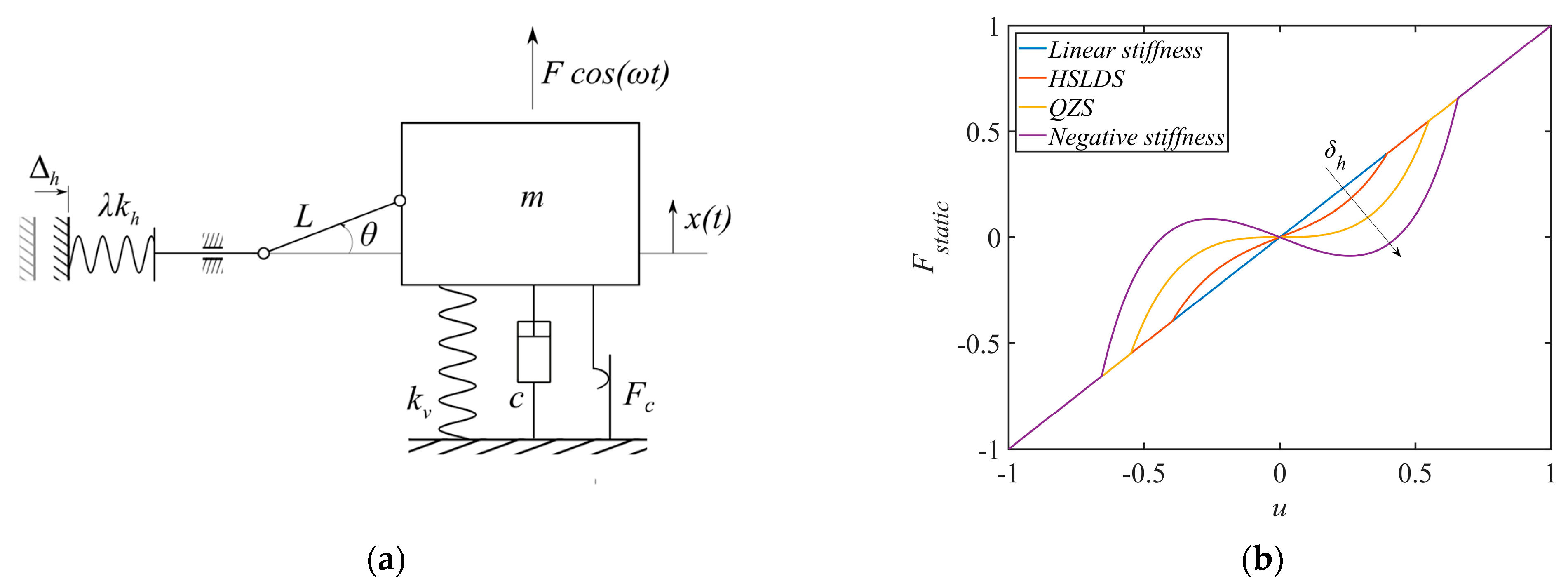
2. Theoretical Formulation

The proposed HSLDS isolator consists of a mass m suspended by a vertical linear spring of stiffness k_v and $\lambda$ linear horizontal springs of stiffness k_h; the displacement Δ_h denotes the horizontal spring preload, L is the length of the oscillating rod, and $\theta$ is the angle between the rod and the horizontal direction. Dissipation phenomena are modelled considering a viscous damper c and a constant dry friction force F_c; the absolute displacement of the mass is given by $x$, and the mass is subject to a harmonic forcing of amplitude F and frequency ω; t is the time variable. A schematic of the system is shown in Figure 1a.

In real applications, compression springs are often used, but they cannot sustain tensile loads. Therefore, when the oscillation amplitude exceeds a critical value $x_{cr}$, it is necessary to account for the detachment of the horizontal springs from the pushrod using a piecewise function to represent the restoring force.

The equation of motion for the isolator shown in Figure 1a incorporating nonlinear stiffness and damping effects is expressed as [39]

$$m\ddot{x}+c\dot{x}+k_{v}x+F_c \mathrm{s}\mathrm{i}\mathrm{g}\mathrm{n}\left(\dot{x}\right)+F_k\left(x\right)=F\mathrm{c}\mathrm{o}\mathrm{s}\left(\omega t\right)$$

(1)

where dots denote time derivatives and $F_k\left(x\right)$ is the nonlinear restoring force with piecewise characteristic. In the case of static equilibrium position with the oscillating rod parallel to the ground ($\theta =0 \mathrm{r}\mathrm{a}\mathrm{d})$, $F_k\left(x\right)$ is given by [14]

$$\begin{gathered} F_k\left(x\right)=\left\{\begin{array}{cc}\lambda k_h\left(L-{\mathsf{\Delta }}_h-\sqrt{L^2-x^2}\right) {\displaystyle \frac{x}{\sqrt{L^2-x^2}}}& \left|x\right|\le \left|x_{cr}\right|\\ 0& \left|x\right|>\left|x_{cr}\right|\end{array}\right. \\ {x}_{cr}=\sqrt{L^2-{\left(L-{\mathsf{\Delta }}_h\right)}^2} \end{gathered}$$

(2)

Dissipation is modeled considering viscous damping and Coulomb dry friction, without possibility of having stick–slip transitions. Therefore, the present formulation is suitable to analyze the system dynamic only in the case of slip conditions, i.e., continuous motion. To study the system’s behavior under stick–slip transitions, enhanced friction models are needed [40,41].

Using a dimensionless notation, Equation (1) is reduced to

$$u^{″}+{2\overline{\zeta }u}^{\prime }+u+\overline{\mu }\mathrm{s}\mathrm{i}\mathrm{g}\mathrm{n}(u^{\prime })+F_k\left(u\right)=F_0\cos \left(\mathsf{\Omega }\tau \right)$$

(3)

where

$$\begin{gathered} {\omega }_n^2={\displaystyle \frac{k_v}{m}},\hspace{1em} \tau ={\omega }_{n}t,\hspace{1em} {\left(·\right)}^{\prime }={\displaystyle \frac{d}{d\tau }},\hspace{1em} \mathsf{\Omega }={\displaystyle \frac{\omega }{{\omega }_n}},\hspace{1em} u={\displaystyle \frac{x}{L}}, \\ {\delta }_h={\displaystyle \frac{{\mathsf{\Delta }}_h}{L}},\hspace{1em} \overline{\zeta }={\displaystyle \frac{c}{2\sqrt{k_{v}m}}},\hspace{1em} \overline{\mu }={\displaystyle \frac{F_c}{k_{v}L}},\hspace{1em} {\overline{F}}_0={\displaystyle \frac{F}{k_{v}L}},\hspace{1em} r={\displaystyle \frac{k_h}{k_v}} \end{gathered}$$

(4)

and the dimensionless nonlinear piecewise restoring force reads as follows:

$$\begin{gathered} {\overline{F}}_k\left(u\right)={\displaystyle \frac{F_k\left(x\right)}{k_{v}L}}=\left\{\begin{array}{cc}\lambda r\left(1-{\delta }_h-\sqrt{1-u^2}\right) {\displaystyle \frac{u}{\sqrt{1-u^2}}}& \left|u\right|\le \left|u_{cr}\right|\\ 0& \left|u\right|>\left|u_{cr}\right|\end{array}\right. \\ {u}_{cr}=\sqrt{1-{\left(1-{\delta }_h\right)}^2} \end{gathered}$$

(5)

Using Taylor’s expansion, the nonlinear restoring force can be approximated as

$${\overline{F}}_k\left(u\right)=\left\{\begin{array}{c}\left(\alpha -1\right)u+\beta u^3+{\gamma u}^5\\ 0\end{array} \begin{array}{c}\left|u\right|\le \left|u_{cr}\right|\\ \left|u\right|>\left|u_{cr}\right|\end{array}\right.$$

(6)

with coefficients derived up to the fifth order

$$\alpha =1-\lambda r{\delta }_h,\hspace{1em} \beta ={\displaystyle \frac{\lambda }{2}}r\left(1-{\delta }_h\right),\hspace{1em} \gamma ={\displaystyle \frac{3}{8}}\lambda r\left(1-{\delta }_h\right)$$

(7)

Due to the symmetry of the system, the restoring force is an odd function [42]; therefore, only odd terms appear in (6). Moreover, the critical deflection $u_{cr}$ is null when the preload ${\delta }_h=0$. This causes the first equation of (5) to collapse into the second, resulting in the restoring force of a linear oscillator. Physically, this is equivalent to isolating the oscillating mass using only the vertical spring.

The static characteristic of the isolator is shown in Figure 1b for different horizontal spring preload ${\delta }_h$: starting from null preload, the restoring force is linear $\left(\overline{\alpha }=1\right)$; while increasing the preload, the behavior changes from High-Static–Low-Dynamic Stiffness $\left(0<\overline{\alpha }<1\right)$ to quasi-zero stiffness $\left(\overline{\alpha }=0\right)$. After quasi-zero-stiffness, the condition of negative stiffness $\left(\overline{\alpha }<0\right)$ occurs at the equilibrium point. Figure 1b shows not only how the stiffness can be tuned by varying ${\delta }_h$, but also the dependence of $u_{cr}$ on ${\delta }_h$: the higher the preload, the larger the range of motion of the isolator that is not affected by detachment. The side effect of a high preload lies in the stiffness at the equilibrium point, which can be negative and resulting in snap-trough mechanism. To this end, a trade-off must be sought to optimize the behavior of such systems, and details are discussed in this paper.

3. Primary Resonance Analysis

3.1. Periodic Motion

The periodic motion in the neighborhood of the primary resonance is analyzed using the Krylov–Bogoliubov–Mitropolsky (KBM) averaging method [36,43]. To this end, Equation (3) is rescaled with respect to a small parameter $ϵ$ [44,45] as

$$u^{″}+{\mathsf{\Omega }}^{2}u=ϵG\left(u,u^{\prime },\mathsf{\Omega }\tau \right)$$

(8)

where

$$G\left(u,u^{\prime },\mathsf{\Omega }\tau \right)=F_0\cos \left(\mathsf{\Omega }\tau \right)-{2\zeta u}^{\prime }-\mu \mathrm{s}\mathrm{i}\mathrm{g}\mathrm{n}\left(u\right)-F_k\left(u\right)+\sigma u$$

(9)

and

$$\overline{\zeta }=ϵ\zeta , \overline{\mu }=ϵ\mu , {\overline{F}}_0=ϵF_0, {\overline{F}}_k=ϵF_k, {\mathsf{\Omega }}^2=1+ϵ\sigma , ϵ\ll 1$$

(10)

$G\left(u,u^{\prime },\mathsf{\Omega }\tau \right)$ is periodic with period $T=2\pi /\mathsf{\Omega }$, and it acts as a perturbation of the underlying linear oscillator.

The first-order approximate solution of (8) is assumed to have slowly varying amplitude $A=A\left(\tau \right)$ and phase $\varphi =\varphi \left(\tau \right)$ as

$$\begin{gathered} u=A\cos \psi \\ {u}^{\prime }=-A\mathsf{\Omega }\sin \psi \end{gathered}$$

(11)

where $\psi =\mathsf{\Omega }\tau +\varphi$.

The time differentiation of the first equation of (11) leads to

$$u^{\prime }=A^{\prime }\cos \psi -A\mathsf{\Omega }\sin \psi -A\varphi \prime \sin \psi$$

(12)

and comparing (12) to the second equation of (11), it requires the following condition to be satisfied:

$$A^{\prime }\cos \psi -A\varphi \prime \sin \psi =0$$

(13)

Differentiating the second equation of (11) gives

$$u^{″}+{\mathsf{\Omega }}^{2}u=-A^{\prime }\mathsf{\Omega }\sin \psi -A\mathsf{\Omega }\varphi \prime \cos \psi$$

(14)

and substituting it into Equation (8) results in

$$A^{\prime }\mathsf{\Omega }\sin \psi +A\mathsf{\Omega }\varphi \prime \cos \psi =-ϵG\left(A\cos \psi ,-A\mathsf{\Omega }\sin \psi ,\psi -\varphi \right)$$

(15)

The set of Equations (13) and (15) is linear with respect to the variables $A^{\prime }$ and $A\varphi \prime$:

$$\left(\begin{array}{cc}\cos \psi & -\sin \psi \\ \sin \psi & \cos \psi \end{array}\right)\left({\displaystyle \genfrac{}{}{0pt}{}{A^{\prime }}{A\varphi \prime }}\right)=\left({\displaystyle \genfrac{}{}{0pt}{}{0}{-\frac{ϵ}{\mathsf{\Omega }}G\left(A\cos \psi ,-A\mathsf{\Omega }\sin \psi ,\psi -\varphi \right)}}\right)$$

(16)

Solving the linear system (16), it is possible to obtain

$$\begin{gathered} A^{\prime }=-{\displaystyle \frac{ϵ}{\mathsf{\Omega }}}G\left(A\cos \psi ,-A\mathsf{\Omega }\sin \psi ,\psi -\varphi \right)\sin \psi \\ A{\varphi }^{\prime }=-{\displaystyle \frac{ϵ}{\mathsf{\Omega }}}G\left(A\cos \psi ,-A\mathsf{\Omega }\sin \psi ,\psi -\varphi \right)\cos \psi \end{gathered}$$

(17)

Averaging System (17) over period $2\pi$, the slow variations of $A$ and $\varphi$ are

$$\begin{gathered} A^{\prime }=-{\displaystyle \frac{ϵ}{2\pi \mathsf{\Omega }}}{\int }_0^{2\pi }G\left(A\cos \psi ,-A\mathsf{\Omega }\sin \psi ,\psi -\varphi \right)\sin \psi d\psi \\ {A\varphi }^{\prime }=-{\displaystyle \frac{ϵ}{2\pi \mathsf{\Omega }}}{\int }_0^{2\pi }G\left(A\cos \psi ,-A\mathsf{\Omega }\sin \psi ,\psi -\varphi \right)\cos \psi d\psi \end{gathered}$$

(18)

System (18) is affected by two nonlinearities: the Coulomb friction and the restoring force. Considering that $u^{\prime }<0 \forall \psi \in \left(0, \pi \right)$ and $u^{\prime }>0 \forall \psi \in \left(\pi ,2\pi \right)$, the modulation Equation (18) is reduced to the standard form:

$$\mathsf{\Gamma }\left(\mathbf{q},\mathsf{\Omega }\right)=\left\{\begin{array}{c}{A}^{\prime }=-{\displaystyle \frac{ϵ}{2\mathsf{\Omega }}}\left(F_0\sin \varphi +2\zeta \mathsf{\Omega }A+{\displaystyle \frac{4}{\pi }}\mu \right)\\ A{\varphi }^{\prime }=-{\displaystyle \frac{ϵ}{2\mathsf{\Omega }}}\left(F_0\cos \varphi +\sigma A+H_i\right)\end{array}\right.$$

(19)

where ${\mathbf{q}}^{\mathbf{T}}=\left[A, \varphi \right]$ and

$$H_i={\displaystyle \frac{1}{2\pi }}{\int }_0^{2\pi }{f}_k\left(A\cos \psi \right)\cos \psi d\psi$$

(20)

with i = 1,2 depending on the value of $A$. If response amplitude $A\le \left|u_{cr}\right|$, the system is not affected by the stiffness discontinuity; thus,

$$H_1=\left(1-\alpha \right)A-{\displaystyle \frac{3}{4}}\beta A^3-{\displaystyle \frac{5}{8}}\gamma A^5$$

(21)

while, if response amplitude $A>\left|u_{cr}\right|$, assuming $u_{cr}=A\cos {\psi }_0$, Integral (20) must be split over four intervals:

• $\left|u\right|\le \left|u_{cr}\right| \forall \psi \in \left[-{\psi }_0,{\psi }_0\right]\cup \left[\pi -{\psi }_0,\pi +{\psi }_0\right]$,
• $\left|u\right|>\left|u_{cr}\right| \forall \psi \in \left[{\psi }_0,\pi -{\psi }_0\right]\cup \left[\pi +{\psi }_0,2\pi -{\psi }_0\right]$.

Hence,

$$\begin{array}{ll}{H}_2=\left(1-\alpha \right)A-& {\displaystyle \frac{3}{4}}\beta A^3-{\displaystyle \frac{5}{8}}\gamma A^5\\ & +{\displaystyle \frac{1}{\pi }}[\left(2\left(\alpha -1\right)A+{\displaystyle \frac{3}{2}}\beta A^3+{\displaystyle \frac{5}{4}}\gamma A^5\right){\psi }_0\\ & +\left(\left(\alpha -1\right)A+\beta A^3+{\displaystyle \frac{15}{16}}\gamma A^5\right)\sin 2{\psi }_0\\ & +\left({\displaystyle \frac{1}{8}}\beta A^3+{\displaystyle \frac{3}{16}}\gamma A^5\right)\sin 4{\psi }_0+{\displaystyle \frac{1}{48}}\gamma A^5\sin 6{\psi }_0]\end{array}$$

(22)

In proximity of the primary resonance, stationary oscillations can be studied from the fixed points of (19) as

$$\begin{gathered} F_0\sin \varphi +2\zeta \mathsf{\Omega }A+{\displaystyle \frac{4}{\pi }}\mu =0 \\ {F}_0\cos \varphi +\sigma A+H_i=0 \end{gathered}$$

(23)

Collecting trigonometric terms at the right-hand-side, squaring and adding side by side, the frequency–response curve is determined as follows:

$$\begin{array}{c}\mathcal{F}\left(\mathsf{\Omega },A\right)=A^2{\mathsf{\Omega }}^4+\left(4A^2{\zeta }^2+2A\left(H_i-A\right)\right){\mathsf{\Omega }}^2+{\displaystyle \frac{16}{\pi }}\mu \zeta A\mathsf{\Omega }+{\displaystyle \frac{16}{{\pi }^2}}{\mu }^2+{\left(H_i-A\right)}^2-F_0^2=0\end{array}$$

(24)

which is a nonlinear algebraic equation. If $\mu \ne 0$, the solution must be obtained numerically while, in the case of negligible Coulomb friction, a closed-form solution can be obtained by solving a quadratic algebraic equation in ${\mathsf{\Omega }}^2$.

The slowly varying phase $\varphi \left(\mathsf{\Omega }\right)$ is retrieved from Equation (23) and it reads as follows:

$$\tan \left(\varphi \right)={\displaystyle \frac{2\mathsf{\zeta }\mathsf{\Omega }A+\frac{4}{\pi }\mu }{\left({\mathsf{\Omega }}^2-1\right)A+H_i}}$$

(25)

Using the definition of Schmidt and Tondl [46], the backbone equation can be obtained from the second equation of (23) by assuming $\cos \left(\varphi \right)=0$ as

$$A_c={\displaystyle \frac{H_i}{1-{\mathsf{\Omega }}^2}}$$

(26)

Further considerations are possible from the evaluation of the critical forcing value to overcome the sticking condition, which can be obtained by the limit envelope under the hypothesis of $A<\left|u_{cr}\right|$ where the isolator is not affected by the restoring force discontinuity. Setting $\sin \left(\varphi \right)=\pm 1$ from the first equation of (23), the limit envelope curve is

$$A_L={\displaystyle \frac{F_0-\frac{4}{\pi }\mu }{2\mathsf{\zeta }\mathsf{\Omega }}}$$

(27)

Analyzing (27), it is possible to recall what is reported in Ref. [46]: in the absence of viscous damping, $\zeta \to 0$, the limit envelope amplitude $A_L\to \infty$; thus, dry friction alone cannot guarantee a bounded response in the case of resonant load with $F_0>{\displaystyle \frac{4}{\pi }}\mu$. If the inequality is not satisfied, the excitation frequency is insufficient to induce vibrations of the isolator; thus, the system lies in the sticking region. The same condition could have been obtained equivalently by imposing $A\to 0$ in the amplitude–frequency Equation (24) as shown in [28].

3.2. Stability

In order to investigate the stability of the fixed points, Equation (19) serves as the basis for the Jacobian matrix evaluation [33] as

$$D_{\mathbf{q}}\mathsf{\Gamma }=\left[\begin{array}{cc}-\zeta & {\displaystyle \frac{1}{2\mathsf{\Omega }}}\left(\sigma A+H_i\right)\\ -{\displaystyle \frac{1}{2\mathsf{\Omega }A}}\left(\sigma +{\displaystyle \frac{\partial H_i}{\partial A}}\right)& -\zeta -{\displaystyle \frac{2\mu }{\pi \mathsf{\Omega }A}}\end{array}\right]$$

(28)

where the characteristic equation is

$${\lambda }^2-\mathrm{t}\mathrm{r}\left(D_{\mathbf{q}}\mathsf{\Gamma }\right)\lambda +\det \left(D_{\mathbf{q}}\mathsf{\Gamma }\right)=0$$

(29)

Since $\mathrm{t}\mathrm{r}\left(D_{\mathbf{q}}\mathsf{\Gamma }\right)<0$, all the eigenvalues have a negative real part; thus, Hopf bifurcations cannot occur. Nevertheless, a static bifurcation (i.e., saddle nodes), as per its definition, can occur if at least one eigenvalue is purely imaginary. Thus, the stability of fixed points can be investigated by finding the values for which $\det \left(D_{\mathbf{q}}\mathsf{\Gamma }\right)$ is null:

$${\mathsf{\Omega }}^4+\left({\displaystyle \frac{H_i}{A}}+{\displaystyle \frac{\partial H_i}{\partial A}}+{4\zeta }^2-2\right){\mathsf{\Omega }}^2+{\displaystyle \frac{8\zeta \mu }{\pi A}}\mathsf{\Omega }+\left(1-{\displaystyle \frac{H_i}{A}}\right)\left(1-{\displaystyle \frac{\partial H_i}{\partial A}}\right)=0$$

(30)

with $H_i$ evaluated according to Equations (21) and (22).

From the analysis of Equation (30), the role played by the dry friction on the stability is marginal and strictly related to the value of the viscous damping ratio. That is, as $\zeta \to 0$, a variation in the dry friction force does not affect the stability boundary.

For the sake of clarity, the derivative of $H_2$ with respect to the oscillation amplitude A is reported as follows:

$$\begin{array}{c}{\displaystyle \frac{\partial H_2}{\partial A}}={\displaystyle \frac{1}{24\pi p}}\left({\displaystyle \frac{16\gamma }{A^3}}{u}_{cr}^7+{\displaystyle \frac{24\beta -20\gamma A^2}{A^3}}{u}_{cr}^5-{\displaystyle \frac{64\left(1-\alpha \right)+2q}{A^3}}{u}_{cr}^3+6{\displaystyle \frac{q}{A}} u_{cr}-3 p q\left(\pi -2{ \psi }_0\right)\right)\end{array}$$

(31)

where

$$\begin{gathered} p=\sqrt{1-{\displaystyle \frac{u_{cr}^2}{A^2}}},\hspace{1em} q=-8+8\alpha +18A^2\beta +25A^4\gamma , \\ { \psi }_0=\arccos \left({\displaystyle \frac{u_{cr}}{A}}\right) \end{gathered}$$

(32)

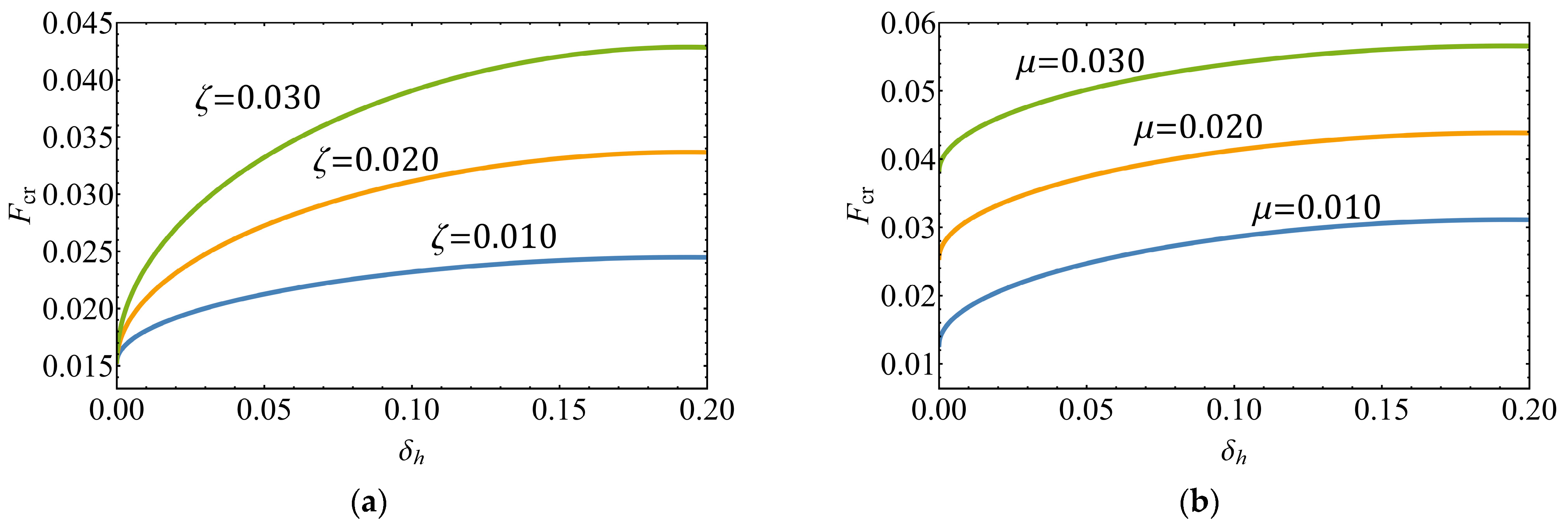
3.3. Critical Forcing Amplitudes F_s and F_cr

It is well known that nonlinear isolators governed by a Duffing-like equation may exhibit saddle-node bifurcations. If the forcing amplitude exceeds a critical value $F_{SN}$, sudden oscillation jumps occur near resonance conditions. To determine the critical forcing value, the approach discussed by Malatkar and Nayfeh [17], based on the Sylvester resultant of two polynomials [47], is adopted here. For excitation amplitudes below the detachment condition, i.e., $A<\left|u_{cr}\right|$, the frequency response displays an inflection point $\left({\mathsf{\Omega }}_s,A_s\right)$, with Equation (24) providing three roots, each counted with its own multiplicity. Considering the derivatives of the frequency–response curve $\mathcal{F}\left(\mathsf{\Omega },A\right)$ with respect the variable $A$, the resultant $\mathcal{R}$, expressed as a function of $\mathsf{\Omega }$, has one positive real root at the inflection point if

$${\left.\mathcal{R}\left({\displaystyle \frac{\partial \mathcal{F}}{\partial A}},{\displaystyle \frac{{\partial }^2\mathcal{F}}{\partial A^2}}\right)\right|}_{A=A_s}=\sum _{\begin{array}{c}i=0,\\ i even\end{array}}^{36}{b}_i{A}_s^i=0$$

(33)

Polynomial (33) can be solved numerically, and the minimum real positive root provides $A_s$. By substituting $A_s$ into ${\displaystyle \frac{{\partial }^2\mathcal{F}}{\partial A^2}}=0$, the critical frequency ${\mathsf{\Omega }}_s$ is obtained. Lastly, the forcing amplitude $F_{SN}$ is provided by the evaluation of $\mathcal{F}\left({\mathsf{\Omega }}_s,A_s\right)=0$.

Another parameter useful to the design of the system is the critical forcing amplitude $F_{cr}$ and frequency ${\mathsf{\Omega }}_{cr}$ leading to the detachment of the horizontal springs from the pushrod, which activates the restoring force piecewise nonlinearity. Those values can be determined by assuming $A=u_{cr}$ within (24) and finding the stationary points of ${\displaystyle \frac{\partial \mathcal{F}}{\partial \mathsf{\Omega }}}=0$, which yields a depressed cubic in $\mathsf{\Omega }$, in which one root identifies the critical value ${\mathsf{\Omega }}_{cr}$. Substituting ${\mathsf{\Omega }}_{cr}$ into (24) leads to an equation of the variable $F_{cr}$. This approach can be easily implemented, but it requires to work with a fixed value of the preload ${\delta }_h$; therefore, it does not show the relationship $F_{cr}=f({\delta }_h$).

A possible approach to determine $F_{cr}=f({\delta }_h$) is applying the Sylvester resultant as follows. Under the assumption of $A=u_{cr}$, the polynomial resultant is constructed from the frequency response curve $\mathcal{F}\left(\mathsf{\Omega },A\right)$ and its first derivative ${\displaystyle \frac{\partial \mathcal{F}}{\partial \mathsf{\Omega }}}$ as

$${\left.\mathcal{R}\left({\left.\mathcal{F}\right|}_{A=u_{cr}},{\left.{\displaystyle \frac{\partial \mathcal{F}}{\partial \mathsf{\Omega }}}\right|}_{A=u_{cr}}\right)\right|}_{\mathsf{\Omega }={\mathsf{\Omega }}_{cr}}=\sum _{\begin{array}{c}i=0,\\ i even\end{array}}^6{c}_i{\left({\delta }_h\right)F}_{cr}^i=0$$

(34)

where $c_i\left({\delta }_h\right)$ represents the ith polynomial in variable ${\delta }_h$. Equation (34) is a nonlinear algebraic equation of variables $F_{cr}$ and ${\delta }_h$. The critical forcing $F_{cr}$ can be determined by using numerical methods by spanning the preload in the range ${\delta }_h\in \left[0,{\left(\lambda r\right)}^{-1}\right]$, which covers a wide range of cases, from HSLDS to the QZS mechanism.

4. Results

In order to investigate the dynamic behavior of the isolator, an additional condition on the restoring force should be of primary concern for this device: the normalized oscillation amplitude cannot be larger than the unit. In fact, if the oscillating rod reaches the vertical position, ($\theta =\pi /2$), the equivalent vertical stiffness is infinite. Since this case is unrealistic and not of practical interest, only cases where $A<1$ are discussed herein.

4.1. Limitations of the First-Order Approximate Solution and Region of Validity

To assess the accuracy of the KBM method, the particular case with linear stiffness (${\delta }_h=0$) and pure Coulomb friction ($\zeta =0, \mu \ne 0$) is initially considered. Den Hartog [22] derived the closed-form solution of the oscillation amplitude under the hypothesis of continuous motion as follows:

$$A=F_0\sqrt{V^2-{\left({\displaystyle \frac{\mu }{F_0}}\right)}^2{U}^2}$$

(35)

and, under the assumption of one-stop per half-cycle, the relationship describing the boundary below which stick–slip phenomena occur is

$$\begin{gathered} A>F_0\sqrt{{\displaystyle \frac{V^2}{1+{\left(\frac{U{\mathsf{\Omega }}^2}{S}\right)}^2}}} \\ V\left(\mathsf{\Omega }\right)={\displaystyle \frac{1}{1-{\mathsf{\Omega }}^2}},\hspace{1em} U\left(\mathsf{\Omega }\right)={\displaystyle \frac{\sin \left(\frac{\pi }{\mathsf{\Omega }}\right)}{\mathsf{\Omega }\left(1+\cos \left(\frac{\pi }{\mathsf{\Omega }}\right)\right)}}, \\ S\left(\mathsf{\Omega }\right)=\underset{0\le \tau \le \pi /\mathsf{\Omega }}{\max }\left[{\displaystyle \frac{\mathsf{\Omega }\sin \left(\tau \right)+U{\mathsf{\Omega }}^2\left(\cos \left(\mathsf{\Omega }\tau \right)+\cos \left(\tau \right)\right)}{\sin \left(\mathsf{\Omega }\tau \right)}}\right] \end{gathered}$$

(36)

where $V\left(\mathsf{\Omega }\right)$ and $U\left(\mathsf{\Omega }\right)$ are known as response and damping functions, respectively. As pointed out in [22], to easily obtain the boundary, it is convenient to notice that $S\ge 1$ for $\mathsf{\Omega }<1/2$, while $S=1$ for $\mathsf{\Omega }>1/2$.

Figure 2a presents the comparison among the analytical solution (35), the KBM and the direct integration method (see Appendix A). For several values of the ratio $\mu /F_0$, the agreement between the numerical and the analytical solutions is excellent. However, the KBM shows discrepancies with the other methods in the case of higher values of $\mu /F_0$, and particularly at low oscillation amplitude. Nevertheless, the qualitative behavior is captured.

A similar observation can be pointed out in Figure 2b where the KBM is compared to direct integration. For low $\mu /F_0$, the averaging method provides a reliable means of studying the qualitative behavior of piecewise nonlinear stiffness isolators in the presence of combined viscous and Coulomb damping. However, caution is required when $\mu /F_0$ is close to the threshold $\pi /4$ that leads to the sticking phenomenon, as identified in Equation (27): in the case of non-smooth nonlinearities, asymptotic methods, such as the KBM, provides approximate expression that are affected by the Gibbs phenomenon. Therefore, in case of high friction and stick–slip behavior, alternative methods, such as direct integration or enhanced HBMs [48,49,50], should be used.

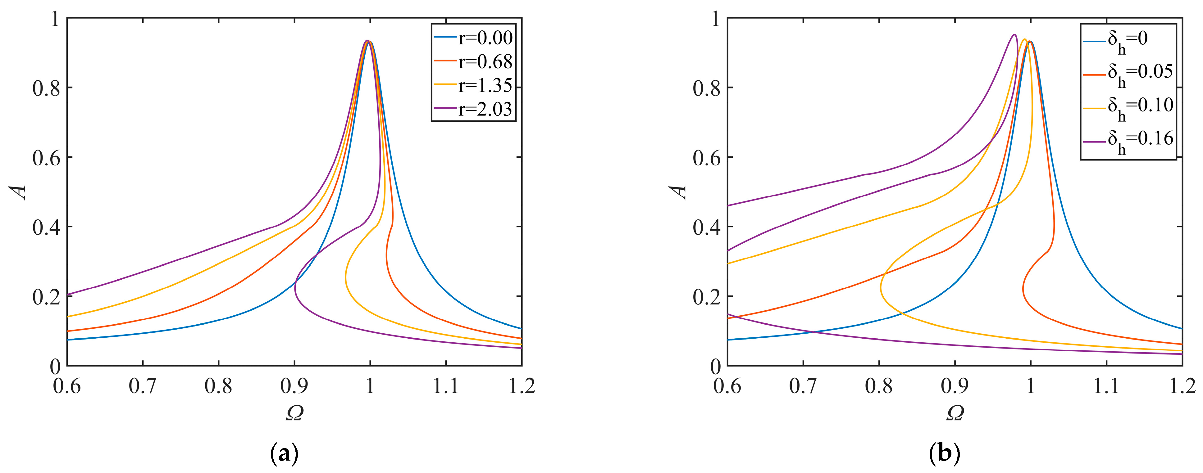
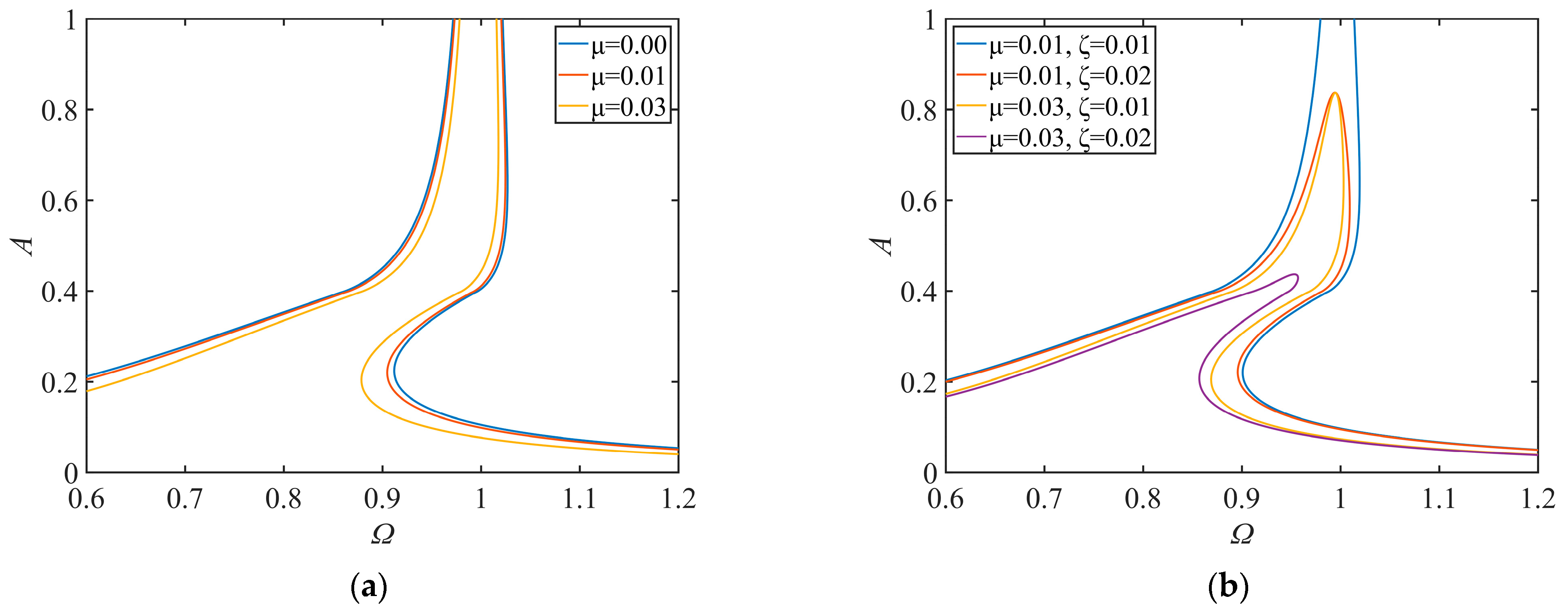
4.2. Parametric Analysis

A parametric analysis is presented here, exploring the effects of stiffness ratio, horizontal spring preload, and damping.

Figure 3a illustrates how the isolator can be tuned by varying the stiffness ratio. Although this may seem intuitive at first glance, it is important to note that, for the mechanism under analysis, this is the only method for modifying the stiffness characteristic without affecting the critical displacement $u_{cr}$. As shown in Figure 3b, where the frequency response is presented by varying the preload ${\delta }_h$ while keeping the stiffness ratio r fixed, the critical displacement $u_{cr}$ is a function of the horizontal spring preload ${\delta }_h$: the higher the preload, the higher is $u_{cr}$. The increment of ${\delta }_h$ yields a secondary effect, which implies a higher critical force $F_{cr}$ that is required to trigger the piecewise behavior of the restoring force.

It is noteworthy that a piecewise nonlinear–linear stiffness mechanisms can also be realized through cam-roller mechanisms [16]. These mechanisms are characterized by a fixed $u_{cr}$, which is determined by the cam profile, and can potentially operate at amplitudes greater than one. This observation is of outmost importance for engineers. Although the equations of motion for both class of HSLDS systems appear similar, the critical condition differs. Hence, when designing a piecewise isolator, it is crucial to be aware of which is the final sought behavior.

Figure 4a,b display the effects of dissipation. According to the limit envelope Equation (27), finite amplitude oscillations at resonance cannot be observed when $\left(\zeta =0,\mu \ne 0 \right)$; see Figure 4a. Specifically, when the threshold value $\mu /F_0>\pi /4$ is exceeded, the external forcing amplitude is insufficient to induce oscillations; thus, $A=0\forall \mathsf{\Omega }$. In contrast, the introduction of viscous damping into the system limits the resonance peak amplitude to finite values, as shown in Figure 4b. Further observations can be made by equating the dissipative terms in the first equation of (23) with those obtained in the case of linear viscous damping. This allows for the determination of an equivalent viscous damping ratio [51]:

$${\mathsf{\zeta }}_{eq}=\zeta +{\displaystyle \frac{2\mu }{\pi \mathsf{\Omega }A}}$$

(37)

in which the role of dry friction is clear; it is negligible near resonance due to the sudden increase in oscillation amplitude, while it becomes significant at low and high forcing frequencies.

The value of the critical forcing determined using the Sylvester resultant (34), which corresponds to the detachment of the horizontal springs from the pushrod, is shown in Figure 5. Specifically, the critical forcing is plotted as a function of the horizontal spring preload for different values of the viscous damping, Figure 5a, and dry friction, Figure 5b. As expected, higher viscous damping $\zeta$ and dry friction forces $\mu$ result in a higher $F_{cr}$, with the critical forcing value reaching a plateau region in the case of the QZS mechanism ${\delta }_h\to {\left(\lambda r\right)}^{-1}$. Notably, the roles played by $\zeta$ and $\mu$ differ as ${\delta }_h\to 0$. Viscous damping has no remarkable effects on the critical forcing, with $F_{cr}$ which tends to $\pi \mu /4$ for any $\zeta$. In contrast, an increment of the dry friction $\mu$ induces a shift toward higher values of $F_{cr}$.

4.3. Numerical Example

In this subsection, a detailed analysis of a specific mechanism is presented, providing an example on how the methods and approximate solutions derived previously can be used for the qualitative design and analysis of the isolator.

The critical deflection $u_{cr}$ and forcing amplitude $F_{cr}$ are key parameters for evaluating the isolator’s behavior. Assuming the parameters listed in

Table 1. Input parameters of the detailed analysis.

$\mathit{\lambda }$	$\mathit{r}$	${\mathit{\delta }}_{\mathit{h}}$	$\mathit{\mu }$	$\mathit{\zeta }$
$3$	${\displaystyle \frac{3747}{1848}}$	${\displaystyle \frac{1}{6r}}$	${\displaystyle \frac{12}{1000}}$	${\displaystyle \frac{2}{100}}$

and using Equations (5) and (34), we obtain $u_{cr}=0.3970$ and $F_{cr}=0.0300$ as indicated by the red dots in Figure 6a,b. Substituting these values into (24) allows for the evaluation of the critical forcing frequency ${\mathsf{\Omega }}_{cr}=0.9288$. The onset of the piecewise restoring force activation is outlined by the black thick lines, beyond which the push-rod detaches from the horizontal spring for any forcing amplitude $F$ within the hatched area. It is important to note that as $u_{cr}$ increases with higher values of ${\delta }_h$, the rate of change in $F_{cr}$ decreases as ${\delta }_h$ approaches ${\left(3r\right)}^{-1}\cong 0.16$. Beyond this threshold, the analysis is no longer of interest to the present study, as it would lead to the emergence of negative stiffness mechanism.

Figure 7a presents the amplitude–frequency diagram for several forcing amplitudes. As shown in the validation analysis, the agreement between the approximate and numerical solution is acceptable. For $F_0\le F_{cr}$, the system behaves as a nonlinear oscillator with quintic stiffness nonlinearity and mixed damping. For $F_0>F_{cr}$, the piecewise nonlinearity of the restoring force is triggered, and the resonance peak shifts toward $\Omega =1$. Using the procedure described in Section 3.2, the Sylvester criterion allows to determine the forcing amplitude $F_{SN}=0.0217$ that prevents the system from experiencing saddle-node bifurcations. For $F_0\le F_{SN}$, the isolator exhibits a predictable behavior without showing response multistability. When $F_0=F_{SN}$, the limit inflection point occurs at $\left({\mathsf{\Omega }}_{SN},A_{SN}\right)=\left(0.7762,0.1825\right)$. For $F_0>F_{SN}$, the stability analysis is carried out to evaluate the occurrence of saddle-node bifurcations, and the jump-up/jump-down frequencies and amplitudes, evaluated using Equations (24) and (30), are listed in

Table 2. Saddle node bifurcation points.

${\mathit{F}}_0$	Jump-Up		Jump-Down
	$\mathit{\Omega }$	$\mathit{A}$	$\mathit{\Omega }$	$\mathit{A}$
$F_{SN}$	-	-	-	-
0.025	0.8023	0.1722	0.8318	0.2893
$F_{cr}$	0.8287	0.1842	0.9288	$u_{cr}$
0.040	0.8672	0.2052	0.9938	0.5536
0.050	0.8976	0.2222	1.0175	0.5876

. In Figure 7b, the phase diagram emphasizes the role of damping. At low forcing amplitude, the phase shift is primarily governed by dissipation while, as the forcing amplitude increases, the phase shift approaches that of an undamped Duffing oscillator.

5. Conclusions

The focus of the present study is to develop an accurate yet simple model to investigate the dynamic behavior of HSLDS isolators. Experimental observations in [14,39] have shown that, depending on the isolator’s design, friction and discontinuous restoring forces significantly influence the vibration mitigation provided by the isolators. Therefore, these factors must be modelled to achieve an accurate representation of real systems. Under the assumption of harmonic load, the primary resonance analysis of HSLDS isolators with piecewise nonlinear–linear stiffness, viscous damping, and dry friction is conducted. Using the Krylov–Bogoliubov–Mitropolsky (KBM) averaging method, the theoretical formulation is derived, with particular attention to the parameters relevant for the design of the isolator. The study validates the KBM approach against closed-form solutions and direct integration of the governing equation, demonstrating its effectiveness in predicting the qualitative system’s behavior.

The conclusions are as follows:

(1) To the best of the author’s knowledge, this study presents the first investigation of the primary resonance analysis of HSLDS isolators with piecewise nonlinear–linear characteristic, viscous damping, and dry friction forces. The findings demonstrate that KBM method is well suited for qualitative analyses, as it provides algebraic equations that can be solved with ease, potentially aiding engineers in the design of systems for vibration isolation.

(2) The parametric analysis shows that, for this type of HSLDS mechanism, increasing the preload of the horizontal springs ${\delta }_h$ has a twofold effect: (i) it reduces the natural frequency of the system and (ii) it increases the critical displacement $u_{cr}$ required to activate the piecewise restoring force. Additionally, a relationship for the equivalent viscous damping is provided, demonstrating the dependence between dry friction, forcing amplitude, and frequency, which explains the limited effect of dry friction near resonance conditions.

(3) The analysis of the Silvester resultant indicates that, regardless of the preload ${\delta }_h$, higher dry friction forces are beneficial in increasing the critical forcing value $F_{cr}$ required to activate the piecewise restoring force nonlinearity. In contrast, increasing viscous damping is effective only at higher ${\delta }_h$ (i.e., for QZS systems), while its effect on $F_{cr}$ is negligible as ${\delta }_h\to 0$.

(4) A detailed analysis, carried out on a specific test case, provides a comprehensive example on how to use the methodology object of the study. Leveraging the Sylvester resultant, critical forcing amplitudes, resulting in the onset of piecewise restoring force, are determined along with the condition to prevent jump-up/jump-down phenomena. Saddle-node bifurcations are determined through the stability analysis, and numerical values are reported in a table for comparison and validation of future studies.

(5) The approach presented herein has two limitations: (i) the adopted friction model is suitable for the analysis of low-friction systems under the assumption of continuous motion; (ii) for friction-to-external force amplitude ratios close to the threshold $\mu /F_0=\pi /4$, KBM performs poorly. In such cases, alternative methods specifically developed to deal with strong and non-smooth nonlinearities may be required [48,49,50].

References

1. Carrella, A.; Brennan, M.J.; Waters, T.P. Static Analysis of a Passive Vibration Isolator with Quasi-Zero-Stiffness Characteristic. J. Sound Vib. 2007, 301, 678–689. [Google Scholar] [CrossRef]
2. Carrella, A.; Brennan, M.J.; Waters, T.P.; Shin, K. On the Design of a High-Static-Low-Dynamic Stiffness Isolator Using Linear Mechanical Springs and Magnets. J. Sound Vib. 2008, 315, 712–720. [Google Scholar] [CrossRef]
3. Carrella, A.; Brennan, M.J.; Waters, T.P.; Lopes, V. Force and Displacement Transmissibility of a Nonlinear Isolator with High-Static-Low-Dynamic-Stiffness. Int. J. Mech. Sci. 2012, 55, 22–29. [Google Scholar] [CrossRef]
4. Brennan, M.J.; Kovacic, I.; Carrella, A.; Waters, T.P. On the Jump-up and Jump-down Frequencies of the Duffing Oscillator. J. Sound Vib. 2008, 318, 1250–1261. [Google Scholar] [CrossRef]
5. Kovacic, I.; Brennan, M.J.; Waters, T.P. A Study of a Nonlinear Vibration Isolator with a Quasi-Zero Stiffness Characteristic. J. Sound Vib. 2008, 315, 700–711. [Google Scholar] [CrossRef]
6. Molyneux, W.G. Supports for Vibration Isolation; Her Majesty’s Stationery Office: London, UK, 1956. [Google Scholar]
7. Platus, D.L. Negative-Stiffness-Mechanism Vibration Isolation Systems. In Proceedings of the Process SPIE 1619, Vibration Control in Microelectronics, Optics, and Metrolog, Los Angeles, CA, USA, 4–6 November 1991; pp. 44–54. [Google Scholar]
8. Shaw, S.W.; Holmes, P.J. A Periodically Forced Piecewise Linear Oscillator. J. Sound Vib. 1983, 90, 129–155. [Google Scholar] [CrossRef]
9. Luo, A.C.J.; Chen, L. Periodic Motions and Grazing in a Harmonically Forced, Piecewise, Linear Oscillator with Impacts. Chaos Solitons Fractals 2005, 24, 567–578. [Google Scholar] [CrossRef]
10. Theodossiades, S.; Natsiavas, S. Periodic and Chaotic Dynamics of Motor-Driven Gear-Pair Systems with Backlash. Chaos Solitons Fractals 2001, 12, 2427–2440. [Google Scholar] [CrossRef]
11. Shaw, S.W. Forced Vibrations of a Beam with One-Sided Amplitude Constraint: Theory and Experiment. J. Sound Vib. 1985, 99, 199–212. [Google Scholar] [CrossRef]
12. Giannini, O.; Casini, P.; Vestroni, F. Experimental Evidence of Bifurcating Nonlinear Normal Modes in Piecewise Linear Systems. Nonlinear Dyn. 2011, 63, 655–666. [Google Scholar] [CrossRef]
13. Ji, J.C.; Hansen, C.H. On the Approximate Solution of a Piecewise Nonlinear Oscillator under Super-Harmonic Resonance. J Sound Vib. 2005, 283, 467–474. [Google Scholar] [CrossRef]
14. Iarriccio, G.; Zippo, A.; Eskandary-Malayery, F.; Ilanko, S.; Mochida, Y.; Mace, B.; Pellicano, F. Tunable High-Static-Low-Dynamic Stiffness Isolator under Harmonic and Seismic Loads. Vibration 2024, 7, 829–843. [Google Scholar] [CrossRef]
15. Narimani, A.; Golnaraghi, M.F.; Jazar, G.N. Sensitivity Analysis of the Frequency Response of a Piecewise Linear System in a Frequency Island. J. Vib. Control 2004, 10, 175–198. [Google Scholar] [CrossRef]
16. Zhou, J.; Wang, X.; Xu, D.; Bishop, S. Nonlinear Dynamic Characteristics of a Quasi-Zero Stiffness Vibration Isolator with Cam-Roller-Spring Mechanisms. J. Sound Vib. 2015, 346, 53–69. [Google Scholar] [CrossRef]
17. Malatkar, P.; Nayfeh, A.H. Calculation of the Jump Frequencies in the Response of s.d.o.f. Non-Linear Systems. J. Sound Vib. 2002, 254, 1005–1011. [Google Scholar] [CrossRef]
18. Yang, J.; Jiang, J.Z.; Neild, S.A. Dynamic Analysis and Performance Evaluation of Nonlinear Inerter-Based Vibration Isolators. Nonlinear Dyn. 2020, 99, 1823–1839. [Google Scholar] [CrossRef]
19. Noh, J.; Yoon, Y.J.; Kim, P. Anhysteretic High-Static–Low-Dynamic Stiffness Vibration Isolators with Tunable Inertial Nonlinearity. Nonlinear Dyn. 2024, 112, 2569–2588. [Google Scholar] [CrossRef]
20. Stanton, S.C.; Culver, D.; Mann, B.P. Tuning Inertial Nonlinearity for Passive Nonlinear Vibration Control. Nonlinear Dyn. 2020, 99, 495–504. [Google Scholar] [CrossRef]
21. Feeny, B.; Guran, A.; Hinrichs, N.; Popp, K. A Historical Review on Dry Friction and Stick-Slip Phenomena. Appl. Mech. Rev. 1998, 51, 321–341. [Google Scholar] [CrossRef]
22. Den Hartog, J.P. Forced Vibrations With Combined Coulomb and Viscous Friction. J. Fluids Eng. 1931, 53, 107–115. [Google Scholar] [CrossRef]
23. Levitan, E.S. Forced Oscillation of a Spring-Mass System Having Combined Coulomb and Viscous Damping. J. Acoust. Soc. Am. 1960, 32, 1265–1269. [Google Scholar] [CrossRef]
24. Pratt, T.K.; Williams, R. Non-Linear Analysis of Stick/Slip Motion. J. Sound Vib. 1981, 74, 531–542. [Google Scholar] [CrossRef]
25. Shaw, S.W. On the Dynamic Response of a System with Dry Friction. J. Sound Vib. 1986, 108, 305–325. [Google Scholar] [CrossRef]
26. Makris, N.; Constantinou, M.C. Analysis of Motion Resisted by Friction. I. Constant Coulomb and Linear/Coulomb Friction. Mech. Struct. Mach. 1991, 19, 477–500. [Google Scholar] [CrossRef]
27. Marino, L.; Cicirello, A.; Hills, D.A. Displacement Transmissibility of a Coulomb Friction Oscillator Subject to Joined Base-Wall Motion. Nonlinear Dyn. 2019, 98, 2595–2612. [Google Scholar] [CrossRef]
28. Ravindra, B.; Mallik, A.K. Hard Duffing-Type Vibration Isolator with Combined Coulomb and Viscous Damping. Int. J. Non-Linear Mech. 1993, 28, 427–440. [Google Scholar] [CrossRef]
29. Detroux, T.; Noël, J.P.; Virgin, L.N.; Kerschen, G. Experimental Study of Isolas in Nonlinear Systems Featuring Modal Interactions. PLoS ONE 2018, 13, e0194452. [Google Scholar] [CrossRef]
30. Habib, G.; Cirillo, G.I.; Kerschen, G. Isolated Resonances and Nonlinear Damping. Nonlinear Dyn. 2018, 93, 979–994. [Google Scholar] [CrossRef]
31. Donmez, A.; Cigeroglu, E.; Ozgen, G.O. An Improved Quasi-Zero Stiffness Vibration Isolation System Utilizing Dry Friction Damping. Nonlinear Dyn. 2020, 101, 107–121. [Google Scholar] [CrossRef]
32. Gao, X.; Teng, H.D. Dynamics and Nonlinear Effects of a Compact Near-Zero Frequency Vibration Isolator with HSLD Stiffness and Fluid Damping Enhancement. Int. J. Non-Linear Mech. 2021, 128, 103632. [Google Scholar] [CrossRef]
33. Nayfeh, A.H.; Balachandran, B. Applied Nonlinear Dynamics: Analytical, Computational, and Experimental Methods; Wiley: Hoboken, NJ, USA, 1995; ISBN 9780471593485. [Google Scholar]
34. Sanders, J.A.; Verhulst, F.; Murdock, J. Averaging Methods in Nonlinear Dynamical Systems; Applied Mathematical Sciences; Springer: New York, NY, USA, 2007; ISBN 978-0-387-48916-2. [Google Scholar]
35. Krylov, N.M.; Bogoliubov, N.N. Introduction to Non-Linear Mechanics; Princeton University Press: Princeton, NJ, USA, 1950; ISBN 9780691079851. [Google Scholar]
36. Bogoliubov, N.N.; Mitropolsky, Y.A. Asymptotic Methods in the Theory of Non-Linear Oscillations; Hindustan Publishing: Delhi, India, 1961. [Google Scholar]
37. Zhang, Y.; Cao, Q. The Recent Advances for an Archetypal Smooth and Discontinuous Oscillator. Int. J. Mech. Sci. 2022, 214, 106904. [Google Scholar] [CrossRef]
38. Liu, C.; Zhang, W.; Yu, K.; Liu, T.; Zheng, Y. Quasi-Zero-Stiffness Vibration Isolation: Designs, Improvements and Applications. Eng. Struct. 2024, 301, 117282. [Google Scholar] [CrossRef]
39. Eskandary-Malayery, F.; Ilanko, S.; Mace, B.; Mochida, Y.; Pellicano, F. Experimental and Numerical Investigation of a Vertical Vibration Isolator for Seismic Applications. Nonlinear Dyn. 2022, 109, 303–322. [Google Scholar] [CrossRef]
40. Berger, E.J. Friction Modeling for Dynamic System Simulation. Appl. Mech. Rev. 2002, 55, 535–577. [Google Scholar] [CrossRef]
41. Pennestrì, E.; Rossi, V.; Salvini, P.; Valentini, P.P. Review and Comparison of Dry Friction Force Models. Nonlinear Dyn. 2016, 83, 1785–1801. [Google Scholar] [CrossRef]
42. Abolfathi, A.; Brennan, M.J.; Waters, T.P.; Tang, B. On the Effects of Mistuning a Force-Excited System Containing a Quasi-Zero-Stiffness Vibration Isolator. J. Vib. Acoust. 2015, 137, 044502. [Google Scholar] [CrossRef]
43. Mitropolskii, Y.A.; Van Dao, N. Applied Asymptotic Methods in Nonlinear Oscillations; Solid Mechanics and Its Applications; Springer: Dordrecht The Netherlands, 1997; ISBN 978-90-481-4865-3. [Google Scholar]
44. Kovacic, I.; Brennan, M.J. The Duffing Equation: Nonlinear Oscillators and Their Behaviour; Kovacic, I., Brennan, M.J., Eds.; Wiley: Hoboken, NJ, USA, 2011; ISBN 9780470715499. [Google Scholar]
45. Mickens, R.E. Truly Nonlinear Oscillations: Harmonic Balance, Parameter Expansions, Iteration, and Averaging Methods; World Scientific: Singapore, 2010; ISBN 978-981-4291-65-1. [Google Scholar]
46. Schmidt, G.; Tondl, A. Non-Linear Vibrations; Cambridge University Press: Cambridge, UK, 1986; ISBN 9780521266987. [Google Scholar]
47. Griffiths, L.W. Introduction to the Theory of Equations; Wiley & Sons: New York, NY, USA, 1947. [Google Scholar]
48. Kim, W.-J.; Perkins, N.C. Harmonic Balance/Galerkin Method for Non-Smooth Dynamic Systems. J. Sound Vib. 2003, 261, 213–224. [Google Scholar] [CrossRef]
49. Schreyer, F.; Leine, R.I. A Mixed Shooting Harmonic Balance Method for Unilaterally Constrained Mechanical Systems. Arch. Mech. Eng. 2016, 63, 297–314. [Google Scholar] [CrossRef]
50. Colaïtis, Y.; Batailly, A. The Harmonic Balance Method with Arc-Length Continuation in Blade-Tip/Casing Contact Problems. J. Sound Vib. 2021, 502, 116070. [Google Scholar] [CrossRef]
51. Bandstra, J.P. Comparison of Equivalent Viscous Damping and Nonlinear Damping in Discrete and Continuous Vibrating Systems. J. Vib. Acoust. Stress Reliab. Des. 1983, 105, 383. [Google Scholar] [CrossRef]
52. Shampine, L.; Reichelt, M. The MATLAB ODE Suite. SIAM J. Sci. Comput. 1997, 18, 1–22. [Google Scholar] [CrossRef]
Figure 1. HSLDS isolator with piecewise nonlinear–linear stiffness, viscous damper and Coulomb friction. (a) Schematic and (b) static characteristics.
Applsci 15 04187 g001
Figure 2. Validation and comparison of the KBM solution. (a) Comparison between Den Hartog’s closed-form solution, KBM, and direct integration for the linear stiffness oscillator in the presence of dry friction only; (b) comparison between KBM and direct integration in the case of λ = 3 , δ h = 6 r 1 , ζ = 0.02 .
Applsci 15 04187 g002
Figure 3. Parametric analysis. (a) Role of the stiffness ratio r, with λ = 3 , δ h = 6 r 1 , ζ = 0.02 , μ = 0.01 , F 0 = 0.05 . (b) Role of the horizontal spring preload δ h , with λ = 3 , r = 2.03 , ζ = 0.02 , μ = 0.01 , F 0 = 0.05 .
Applsci 15 04187 g003
Figure 4. Parametric analysis. (a) Role of the dry friction force μ, with λ = 3 , r = 2.03 , δ h = 6 r 1 , ζ = 0 , F 0 = 0.05 . (b) Mixed damping conditions, with λ = 3 , r = 2.03 , δ h = 6 r 1 , F 0 = 0.05 .
Applsci 15 04187 g004
Figure 5. Critical forcing amplitude F c r as a function of the horizontal spring preload δ h . (a) Role of the viscous damping, with λ = 3 , r = 2.03 , μ = 0.012 ; (b) role of the dry friction force μ , with λ = 3 , r = 2.03 , ζ = 0.02 .
Applsci 15 04187 g005
Figure 6. Evaluation of the critical (a) displacement u c r and (b) forcing amplitude F c r with the set of parameters given in Table 1.
Applsci 15 04187 g006
Figure 7. Steady-state dynamic response of the oscillator for different forcing amplitude vales F0. (a) Amplitude–frequency curves and stability region and, (b) phase.
Applsci 15 04187 g007