Hyper-CycleGAN: A New Adversarial Neural Network Architecture for Cross-Domain Hyperspectral Data Generation

Abstract

The scarcity of labeled training samples poses a significant challenge in hyperspectral image classification. Cross-scene classification has been shown to be an effective approach to tackle the problem of limited sample learning. This paper investigates the usage of generative adversarial networks (GANs) to enable collaborative artificial intelligence learning on hyperspectral datasets. We propose and design a specialized architecture, termed Hyper-CycleGAN, for heterogeneous transfer learning across source and target scenes. This architecture enables the establishment of bidirectional mappings through efficient adversarial training and merges both source-to-target and target-to-source generators. The proposed Hyper-CycleGAN architecture harnesses the strengths of GANs, along with custom modifications like the integration of multi-scale attention mechanisms to enhance feature learning capabilities specifically tailored for hyperspectral data. To address training instability, the Wasserstein generative adversarial network with gradient penalty (WGAN-GP) loss discriminator is utilized. Additionally, a label smoothing technique is introduced to enhance the generalization capability of the generator, particularly in handling unlabeled samples, thus improving model robustness. Experimental results are performed to validate and confirm the effectiveness of the cross-domain Hyper-CycleGAN approach by demonstrating its applicability to two real-world cross-scene hyperspectral image datasets. Addressing the challenge of limited labeled samples in hyperspectral image classification, this research makes significant contributions and gives valuable insights for remote sensing, environmental monitoring, and medical imaging applications.

1. Introduction

Hyperspectral images (HSI) consist of continuous, narrow spectral bands, reflecting not only the spatial information but also the spectral information of remotely sensed objects. With high-resolution spectral information and large-scale spatial information, hyperspectral images have demonstrated outstanding capabilities in many fields, such as geological exploration and medicine [1]. Hyperspectral image classification is an important application. Many machine learning algorithms have been designed and applied to HSI classification. However, the small sample problem still makes HSI classification very challenging.

In the past few years, many deep-learning-based HSI classification methods have achieved impressive results. The authors of [2] proposed a spectral attention network that purposefully suppresses less useful spectral bands and enhances valuable spectral bands to solve the HSI classification problem. In the work of Shen et al. [3], a deep fully convolutional network (FCN) was utilized to take the entire data cube of an HSI as an input, which can then effectively integrate long-range contextual information. The authors of [4] designed a convolutional neural network (CNN)-based network that can merge features at multiple scales. However, CNNs can only handle relationships in spatial neighborhoods. The authors of [5] proposed a deep feature aggregation framework driven by a graph convolutional network (DFAGCN) model. The model first extracts features using CNN and then introduces a GCN-based model [6] and, finally, fuses the features using a weighted concatenation method. The authors of [7] proposed small-batch GCN (miniGCN), which trains the network in small batches, extracts different features using CNN and miniGCN, and fuses the features using three fusion strategies for HSI classification. However, most methods based on deep learning theory require a sufficient number of labeled samples for training, otherwise it is difficult to achieve the desired classification results. Unfortunately, off-the-shelf labeled hyperspectral images are rare, and labeling new images can be both time-consuming and expensive [8].

A promising alternative direction lies in cross-domain generation of hyperspectral data. To improve the classification performance of a dataset with a limited number of labeled samples (called the target scene), we can use information from another similar dataset with sufficient labeled samples (called the source scene) [9]. However, due to different imaging sensors, the source and target scenes may contain different feature distributions, which leads to a non-negligible classification problem. There is also a large amount of distortion and noise on the generated hyperspectral data.

In recent years, models based on generative adversarial networks (GANs) [10] have been used for migration learning in remote sensing. GANs can generate fake samples that are indistinguishable from the real ones. Typically, a GAN-based model consists of a generator and a discriminator. It is relatively feasible to transfer images from one scene to another by adversarial learning [11]. The auxiliary classifier GAN (AC-GAN) [12] introduces labeling information into the training process of GAN. Another approach, CycleGAN (the cycle-consistent generative adversarial network), was proposed by Zhu et al. [13] and is a modified model of GAN that creates a bidirectional mapping between two different scenes. Many GAN-based methods achieve alignment of cross-scene feature distributions by minimizing domain differences [14].

In this paper, we propose and design a novel adversarial neural network architecture for cross-domain data generation, termed Hyper-CycleGAN, which is targeted toward hyperspectral data. Specifically, the Hyper-CycleGAN architecture makes the following contributions:

• The architecture initiates with a bidirectional mapping network to ensure consistency in data distribution between source and target scenes. These generators are shared within the system to guarantee cyclic consistency and enable efficient reconstruction of samples mapped across domains. Despite improved model performance, it is observed that the data generated by the original CycleGAN generator exhibit noise and poor quality, with a lack of detailed features.
• Consequently, modifications are made to the original internal module of the generator by incorporating a multi-scale attention mechanism. This adjustment allows for an enhanced capture of subtle relationships between spectral bands, prioritization of salient spectral features, and consideration of the spatial distribution of spectral information.
• The discriminator employs the PatchGAN [15] architecture for local feature analysis, enhancing detail and structure recognition in hyperspectral images. Meanwhile, the Wasserstein GAN with gradient penalty (WGAN-GP) [16] technique is utilized to stabilize the training process and improve both fidelity and quality of the synthetic hyperspectral data.
• A hyperspectral data evaluation tool based on the ResNet architecture is subsequently created. This tool employs a complex structure consisting of ResBlocks [17] and DenseBlocks [18] to efficiently capture and interpret the rich spectral information in each hyperspectral data sample, ensuring its performance in processing hyperspectral data analysis tasks and its robustness in processing these tasks.

In summary, our proposed Hyper-CycleGAN architecture harnesses the strengths of CycleGAN, along with custom modifications like the integration of multi-scale attention mechanisms [19], to enhance feature learning capabilities specifically tailored for hyperspectral data. This results in a more robust and efficient image transformation model capable of generating high-quality, realistic hyperspectral data while improving details and reducing noise. Experimental results validate the superiority of our Hyper-CycleGAN architecture over traditional approaches, demonstrating enhanced recognition performance across diverse scenarios from the perspective of hyperspectral data analysis.

2. Background

In this section, we provide the related topics in brief, including deep learning for hyperspectral data and adversarial neural networks for hyperspectral data, to give readers the background for better understanding.

2.1. Deep Learning for Hyperspectral Data

Hyperspectral data, as noted by Mehta et al. [20], differs significantly from traditional RGB imaging by capturing detailed information across numerous narrow spectral bands rather than just three broad ones. This enables precise differentiation of subtle material variations but also introduces challenges due to its high dimensionality and complexity, necessitating specialized mathematical and computational approaches for effective analysis. Researchers have applied numerous machine learning techniques to extract valuable information from these complex datasets [21]. Traditional methods have shown considerable effectiveness in hyperspectral data analysis across various applications. Techniques such as spectral indices and band ratios offer computationally efficient solutions for identifying specific materials [22]. Dimensionality reduction approaches, including principal component analysis (PCA) and independent component analysis (ICA), effectively preserve essential information while reducing data complexity [23]. Furthermore, conventional classifiers, like support vector machines (SVMs) [24] and random forests, demonstrate strong performance in hyperspectral classification, particularly when training samples are limited [25]. These traditional methods typically require fewer computational resources and perform exceptionally well when analyzing materials with well-defined spectral signatures.

A significant challenge in hyperspectral imaging applications stems from the combination of limited training samples and extensive feature sets, making reliable statistical parameter estimation difficult. While traditional methods perform admirably in scenarios with clear spectral separation, they often struggle with complex scenes containing mixed pixels and subtle spectral variations [26]. Deep learning approaches offer complementary capabilities that address these limitations, particularly for applications requiring automated feature extraction from complex datasets. Hyperspectral image classification represents a domain where deep learning has made substantial advances. Unlike conventional methods that rely on manually engineered features and may struggle to capture intricate patterns in hyperspectral data [27], deep learning models automatically learn hierarchical representations from raw data. Convolutional neural networks (CNNs) [28] and recurrent neural networks (RNNs) [29] have demonstrated superior classification accuracy for complex scenes through this automated feature learning capability.

The optimal choice between traditional and deep learning approaches depends on specific application requirements, training data availability, and computational constraints. For example, both traditional mathematical models [30] and deep learning architectures [7] have successfully addressed spectral unmixing tasks. Similarly, anomaly detection benefits from both statistical approaches [31] and deep autoencoder networks [32]. This paper presents a deep-learning-based adversarial neural network architecture for hyperspectral image classification, while acknowledging that traditional methods maintain significant relevance in specific application contexts.

2.2. Adversarial Neural Networks for Hyperspectral Data

In the context of deep learning for hyperspectral data processing, acquiring a substantial volume of labeled data to train supervised learning models presents a significant challenge due to the complexity and diversity of hyperspectral data, which escalates the cost of labeled data acquisition. As Wang et al. [33] pointed out in their research, this challenge has prompted researchers to explore unsupervised learning methods, particularly heterogeneous domain adaptation techniques for hyperspectral image classification. Similarly, Reddy et al. [34] emphasized the difficulty of acquiring labeled data in hyperspectral image processing. To address these challenges, adversarial neural networks have emerged as a viable solution. These networks can be trained without labeled data, learning the distribution and features of data in an unsupervised or semi-supervised manner. Primitive GANs operate adversarially, where the generator network produces realistic hyperspectral data samples, while the discriminator network distinguishes between generated and real data, encouraging the generator to produce increasingly realistic samples. The cycle-consistent generative adversarial network (CycleGAN) [13], a specialized architecture within adversarial neural networks, facilitates domain transformation without requiring paired training data. Recent research has demonstrated CycleGAN’s significant potential in hyperspectral data processing. Chen et al. [35] proposed a CycleGAN-based hyperspectral image super-resolution reconstruction method, while Zhao et al. [36] explored using CycleGAN for hyperspectral image denoising and feature enhancement, providing new insights for unsupervised hyperspectral data processing. For data conversion, let s ∈ R^W×H×B and t ∈ R^W×H×B be features belonging to the source and target scenes, respectively. Here, W × H is the spatial dimension, and B is the spectral dimension. Then, the aim of CycleGAN is to learn the mapping from G_S→T and G_T→S. Overall, CycleGAN consists of two generators, $G_{S\to T}$ and $G_{T\to S}$, and two discriminators, $D_S$ and $D_T$. CycleGAN uses three different loss functions to perform the transformation task, and they are as follows:

Adversarial loss: it aims to transform samples in the source domain into samples in the target domain and will learn the mapping S→T, i.e., $G_{S\to T}\left(s\right)$:

$$\begin{array}{c}{\mathcal{L}}_{adv}\left(G_{S\to T},D_T\right)={\mathbb{E}}_{t\sim T\left(t\right)}\left[log{D}_T\left(t\right)\right]\\ \hspace{1em}\hspace{1em}\hspace{1em}\hspace{1em}\hspace{1em}\hspace{1em}\hspace{1em}\hspace{1em}\hspace{1em}\hspace{1em}\hspace{1em} +{\mathbb{E}}_{S\sim P_S\left(s\right)}\left[\mathit{log}\left(1-D_T\left(G_{S\to T}\left(s\right)\right)\right)\right]\end{array}$$

(1)

Cycle-consistency loss: it aims to retain its original feature vectors using periodic losses to ensure that the network is able to learn both the forward and inverse mappings:

$$\begin{array}{c}{\mathcal{L}}_{cyc}\left(G_{S\to T},G_{T\to S}\right)\\ \hspace{1em}\hspace{1em}\hspace{1em}\hspace{1em}\hspace{1em}\hspace{1em}\hspace{1em}\hspace{1em}\hspace{1em}\hspace{1em} ={\mathbb{E}}_{s\sim P_S\left(s\right)}\left[{∥G_{T\to S}\left(G_{S\to T}\left(s\right)\right)-s∥}_1\right]\mid \\ \hspace{1em}\hspace{1em}\hspace{1em}\hspace{1em}\hspace{1em}\hspace{1em}\hspace{1em}\hspace{1em}\hspace{1em}\hspace{1em}\hspace{1em}\hspace{1em}\hspace{1em} +{\mathbb{E}}_{t\sim P_T\left(t\right)}\left[{∥G_{S\to T}\left(G_{T\to S}\left(t\right)\right)-t∥}_1\right]\end{array} ,$$

(2)

where ||.||₁ is the L₁-norm and $\mathbb{E}$ [.] is the expectation operator.

Identity-mapping loss: It is used to preserve the identity of the target class in the network. It is generally employed to train the network for initial learning, i.e.,

$$\begin{array}{c}{\mathcal{L}}_{id}\left(G_{S\to T},G_{T\to S}\right)={\mathbb{E}}_{s\sim P_S\left(s\right)}\left[{∥G_{T\to S}\left(s\right)-s∥}_1\right]\\ \hspace{1em}\hspace{1em}\hspace{1em}\hspace{1em}\hspace{1em}\hspace{1em} \hspace{1em}+{\mathbb{E}}_{t\sim T\left(t\right)}\left[{∥G_{S\to T}\left(t\right)-t∥}_1\right]\end{array}$$

(3)

Full objective: the overall objective of the CycleGAN network is given as:

$$\begin{array}{c}{\mathcal{L}}_{\mathrm{full} }={\lambda }_{\mathrm{adv} }{\mathcal{L}}_{\mathrm{adv} }\left(G_{S\to T},D_T\right)+{\lambda }_{\mathrm{adv} }{\mathcal{L}}_{adv}\left(G_{T\to S},D_S\right)\\ +{\lambda }_{\mathrm{cyc} }{\mathcal{L}}_{\mathrm{cyc} }\left(G_{S\to T},G_{T\to S}\right)\\ +{\lambda }_{id}{\mathcal{L}}_{id}\left(G_{S\to T},G_{T\to S}\right),\end{array}$$

(4)

where ${\lambda }_{\mathrm{adv} }$, ${\lambda }_{\mathrm{cyc} }$, and ${\lambda }_{id}$ are the weights associated with adversarial, cycle-consistency, and identity-mapping loss, respectively. These values are used as hyperparameters in the network during training.

3. The Proposed Hyper-CycleGAN

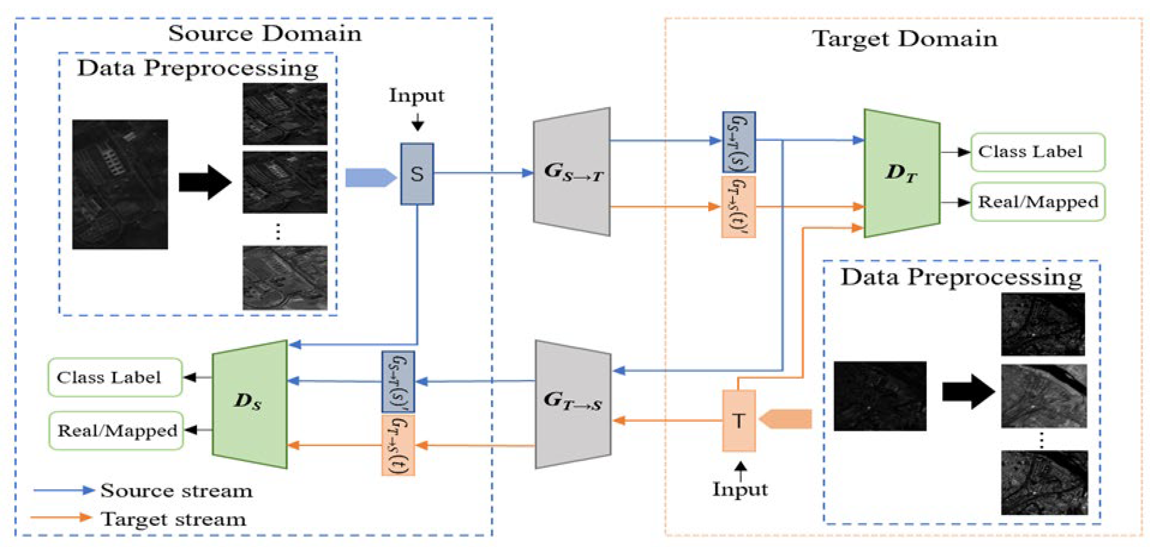
The proposed Hyper-CycleGAN architecture was designed to classify spectral information. In this architecture, the CycleGAN cycle network was adapted, with specific adjustments, as illustrated in Figure 1. This architecture comprises two streams: the target stream (indicated by orange lines) traverses from the target scene through the source scene and back, whereas the source stream (indicated by blue lines) follows a reverse path. Transforming original images into those of other scenes enables the generation of new hyperspectral data. However, it was observed that images generated by the original CycleGAN generator were marred by noise and poor quality, with a lack of detail. Consequently, the internal modules of the generator were modified, notably through the incorporation of a multi-scale attention mechanism. This mechanism enables the network to concentrate on various parts of the image at differing scales, thus more effectively capturing the details and features characteristic of hyperspectral images.

Generator: Figure 2 depicts the proposed architecture, highlighting the internal configuration of the specially designed Hyper-CycleGAN generator module. Internally, the Hyper-CycleGAN generator’s architecture employs an encoder–decoder framework consisting of three primary components: an encoder, a multi-scale attention module, and a decoder. The encoder functions by transforming the input image into an intermediary representation or feature vector, typically utilizing multiple convolutional layers to extract features at various levels within the image. Designed to capture inter-band correlations, the multi-scale attention module amplifies focus on specific spectral attributes and enhances understanding of spectral spatial information, thus improving the quality and precision of generated hyperspectral data. Conversely, the decoder component reverses the encoding process, translating the feature vector back into an image within the target domain through multiple inverse convolutional layers tasked with rendering the feature vector into the final image within said domain.

Algorithm 1 delineates the pseudocode framework for the integration of a multi-scale attention module within the bespoke architecture of the Hyper-CycleGAN module, specifically devised for the synthesis of hyperspectral data. Our methodology is predicated on addressing the unique challenges intrinsic to hyperspectral data, by maintaining the original generator’s capacity to discern and assimilate complex mapping relationships among hyperspectral images. This foundational principle is critical for ensuring the generator’s ongoing effectiveness in enabling seamless transformations across diverse spectral domains.

To elevate the quality and complexity of the synthesized hyperspectral data, we have introduced multi-scale attention modules. These modules are meticulously designed to enhance the generator’s perceptual sharpness and contextual comprehension within the hyperspectral domain. Their design aims to identify correlations between varying wavelengths, focus attention on specific spectral features, and deepen the understanding of spectral spatial information. The intricate interplay between spectral bands is revealed through subtle variations and correlations across different wavelengths. Such interplay might include dependencies between adjacent spectral bands, illustrating how alterations in one band could affect the attributes of neighboring bands. Furthermore, spectral bands may engage in complex interactions, such as absorption and emission patterns, contributing to the scene’s overall spectral signature. The emphasis on prominent spectral features within the multi-scale attention modules is evidenced by the selective amplification of specific spectral components identified as vital for the synthesis process. This entails focusing on distinctive spectral peaks or valleys that correlate with specific materials or substances in the scene. By prioritizing these essential spectral features, the generator can accurately capture the fundamental characteristics of the hyperspectral data, leading to more precise synthesis outcomes.

Algorithm 1: Hyper-CycleGAN generator with multi-scale attention pseudocode

1: inputs (), down_stack (), up_stack (), last ()   2: outputs ()   3: x ← inputs   4: skips ← []   5: for down in down_stack do   6:    x ← down(x)   7:    skips.append(x)   8: end for   9: skips ← reversed(skips[: −1]) 10: for up, skip in zip(up_stack, skips) do 11:    x ← self_attention(x) {} 12:    attention_outputs ← [] 13:    for i do 14:    scaled_input ← Conv1D(x, filters = x.shape[−1], kernel_size = i + 1, padding = ‘same’) {} 15:    attention_output ← MultiHeadAttention(scaled_input, scaled_input) {} 16:    attention_outputs.append(attention_output) 17:    end for 18:    merged_attention ← Concatenate(attention_outputs) {} 19:    x ← Concatenate([x, merged_attention]) {} 20:    x ← up(x) 21:    x ← Concatenate()([x, skip]) 22: end for 23: outputs ← last(x) 24: return outputs

Moreover, integrating spatial contextual cues into the framework fosters a deeper comprehension of the spatial distribution of spectral information. This requires examining how spectral characteristics vary across different spatial locations within a scene. For instance, the spatial arrangement of vegetation, water bodies, or built structures may reveal unique spectral signatures that contribute to the scene’s overall spectral composition. Incorporating spatial contextual information allows the generator to better situate spectral features within their spatial contexts, resulting in more realistic and contextually relevant synthesis outcomes.

In summary, incorporating multi-scale attention modules significantly enhances the Hyper-CycleGAN framework’s capability to synthesize high-quality hyperspectral data. This enhancement facilitates capturing the subtle relationships between spectral bands, prioritizing salient spectral features, and considering the spatial distribution of spectral information. Consequently, this advancement propels the state-of-the-art in hyperspectral data synthesis forward.

Discriminator: The discriminator’s role in hyperspectral data analysis is pivotal for distinguishing between real and synthetically generated hyperspectral data. It scrutinizes the data’s features, identifying genuine hyperspectral characteristics in the actual data while pinpointing discrepancies in the generated data. This discernment capability renders the discriminator an integral component in the training regimen of the generator. In our research, we selected PatchGAN as the foundational architecture for the discriminator module, explicitly optimized for hyperspectral data examination. PatchGAN employs convolutional neural networks (CNNs) to impose specific penalties on N*N feature blocks. Within this architectural framework, CNNs serve as the terminal layers, methodically segmenting the input hyperspectral image into discrete blocks or patches. This segmentation facilitates the independent assessment of each patch, enabling a localized scrutiny of spectral features. By concentrating on smaller segments of the hyperspectral image, PatchGAN not only simplifies the model’s complexity but also enables a more detailed analysis of localized image attributes. Such localized scrutiny significantly augments the framework’s proficiency in capturing the subtle details and structural intricacies inherent to hyperspectral data. Consequently, integrating PatchGAN into our methodology substantially enhanced our ability to discern complex spectral patterns and spatial interrelations within hyperspectral images, thereby improving hyperspectral data analysis and interpretation.

Furthermore, to address potential training challenges and augment overall performance in hyperspectral data analysis, we incorporated Wasserstein GAN with gradient penalty (WGAN-GP) into our discriminator architecture. WGAN-GP is instrumental in refining hyperspectral data synthesis by tackling specific challenges inherent to the generation process. The essence of WGAN-GP lies in the introduction of a gradient penalty term, which applies constraints to the gradient architecture of the generated hyperspectral samples. This constraint effectively moderates the gradient, thus stabilizing the training process and facilitating the generation of more realistic hyperspectral data. WGAN-GP is crucial for overcoming issues related to gradient instability, such as gradient explosion or vanishing gradients, which pose significant challenges in hyperspectral data synthesis. By managing the gradient, WGAN-GP ensures more consistent training dynamics, culminating in enhanced efficiency in data synthesis and superior capabilities in data reconstruction and denoising. Mathematically, the loss function of WGAN-GP can be expressed as:

$$\begin{array}{c}{\mathcal{L}}_{\mathrm{W}\mathrm{G}\mathrm{A}\mathrm{N}-\mathrm{G}\mathrm{P}}\left({\mathrm{D}}_{\mathrm{S}}\right)={\mathbb{E}}_{\widehat{\mathrm{s}}\sim {\mathrm{P}}_{\tilde{\mathrm{s}}}}\left[D\right(\widehat{\mathrm{s}}\left)\right]-{\mathbb{E}}_{\mathrm{s}\sim {\mathrm{P}}_{\mathrm{s}}}\left[D\right(s\left)\right]\\ +\lambda {\mathbb{E}}_{\tilde{\mathrm{s}}\sim {\mathrm{P}}_{\tilde{\mathrm{s}}}}\left[\left({∥{\nabla }_{\tilde{\mathrm{s}}}\mathrm{D}\left(\tilde{\mathrm{s}}\right)∥}_2-\right.\right.\left.1{)}^2\right]\end{array}$$

(5)

Here, D_S still denotes the discriminator, $P_{\tilde{s}}$ is the distribution formed by a mixture of real and generated data, λ is the weight of the gradient penalty term, and $\widehat{s}$ is a sample sampled from $P_{\tilde{s}}$, a distribution formed by linear interpolation between real and generated data. The incorporation of a gradient penalty term in the Wasserstein generative adversarial network with gradient penalty (WGAN-GP) incentivizes the discriminator to acquire smoother and more stable decision boundaries throughout the training process. This augmentation leads to a substantial enhancement in the training efficiency of the model and elevates the quality of the generated samples.

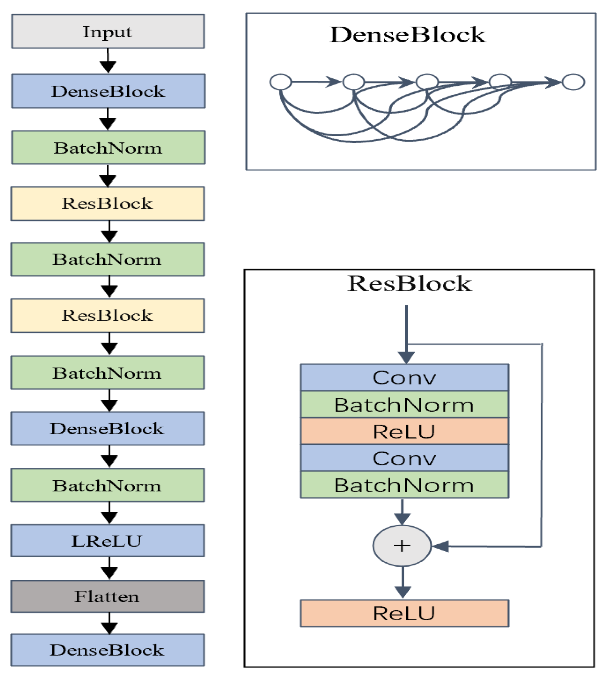
Hyper-CycleGAN classifier: Upon the generation of new hyperspectral data by the generator, our subsequent endeavor involved the development of a ResNet classifier to rigorously evaluate the quality and fidelity of the generated data. Figure 3 delineates the detailed architecture of our meticulously designed classifier, which was specifically crafted to examine the spectral signatures embedded within the synthesized hyperspectral dataset.

At the heart of our hyperspectral classifier model resides a custom amalgamation of residual blocks (ResBlocks) and dense blocks (DenseBlocks), each meticulously engineered to navigate the intricacies and complexities inherent in hyperspectral data analysis. These architectural elements formed the foundation of our classifier, empowering it to adeptly capture and interpret the rich spectral information contained within each hyperspectral data sample. Within the ResBlocks, our classifier utilized the strength of residual connections to ensure unimpeded information flow and gradient propagation, thereby facilitating effective feature extraction and representation learning. The employment of these residual connections allowed our classifier to effectively counteract the vanishing gradient issue, a common challenge in deep neural networks, thus enhancing its capacity to detect subtle spectral variations and intricate patterns inherent in hyperspectral data. Complementing the ResBlocks, the DenseBlocks are distinguished by their dense connectivity patterns, which enhance feature reuse and enable the extraction of highly discriminative spectral features. Through this dense connectivity, our classifier was poised to harness the extensive spectral information available across different wavelengths, thereby enabling precise discrimination of subtle spectral nuances and accurate classification of hyperspectral data samples.

Moreover, the architecture of our hyperspectral classifier was thoughtfully designed to include spectral-specific layers and operations, ensuring its suitability for tasks associated with hyperspectral data analysis. These spectral-specific adaptations permitted our classifier to effectively capture the unique spectral characteristics intrinsic to hyperspectral imagery, thereby augmenting its overall efficacy and robustness in hyperspectral data classification tasks.

Hyper-CycleGAN training: Algorithm 2 shows the Hyper-CycleGAN training pseudocode. Our training was divided into two parts: generator–discriminator training and classifier training. In the generator–discriminator training part, two generators and two discriminators were trained simultaneously in an adversarial manner [37]. First, for ${\mathcal{L}}_{\mathrm{a}\mathrm{d}\mathrm{v}}$ (Equation (1)), we replaced the negative log-likelihood objective with a least squares loss [38]. This loss was more stable during training and produced higher-quality results. In particular, for the GAN loss ${\mathcal{L}}_{\mathrm{a}\mathrm{d}\mathrm{v}}\left({\mathrm{G}}_{\mathrm{S}\to \mathrm{T}},{\mathrm{D}}_{\mathrm{T}}\right)$, we trained G to minimize ${\mathbb{E}}_{\mathrm{t}\sim \mathrm{T}\left(\mathrm{t}\right)}\left[\mathrm{l}\mathrm{o}\mathrm{g}{\mathrm{D}}_{\mathrm{T}}\left(\mathrm{t}\right)\right]$ and trained D to minimize ${\mathbb{E}}_{\mathrm{S}\sim {\mathrm{P}}_{\mathrm{S}}\left(\mathrm{s}\right)}\left[\log \left(1-{\mathrm{D}}_{\mathrm{T}}\left({\mathrm{G}}_{\mathrm{S}\to \mathrm{T}}\left(\mathrm{s}\right)\right)\right)\right]$.

Secondly, to mitigate model oscillations and optimize training for hyperspectral data synthesis, we incorporated a strategy proposed in [39]. This strategy involved updating the discriminator using a history of previously generated hyperspectral images rather than the most recent ones. An image buffer was maintained to store the 60,000 previously generated hyperspectral samples. Moreover, we introduced label smoothing during the training process to enhance model robustness and generalization capability, particularly in the context of hyperspectral data. Label smoothing involves adjusting the target labels for real and fake samples to encourage more calibrated and confident predictions from the discriminator. This regularization technique prevents the discriminator from becoming overly confident in its predictions and fosters the generation of diverse and realistic hyperspectral outputs, essential for accurate and reliable hyperspectral data synthesis.

During the classifier training phase, our focus shifted to harnessing the unique spectral characteristics inherent in hyperspectral data for effective classification tasks. Leveraging ResNet, specifically tailored for hyperspectral data analysis, we embarked on a journey to decode the complex spectral signatures embedded within our synthesized dataset. This dataset, meticulously crafted by the generator, served as the cornerstone of our classifier’s training regimen. In the initial stages, as we laid the foundation for our ResNet model, we carefully initialized the weight parameters using the common random initialization method. This ensured that our classifier possessed the versatility to capture the rich and intricate spectral features encapsulated within hyperspectral data cubes. By imbuing our model with this innate adaptability, we equipped it with the capability to navigate the vast expanse of spectral space with precision and finesse. Optimization became paramount as we delved deeper into the training process. Here, we made a deliberate choice in favor of the Adam optimizer, renowned for its efficacy in handling the inherent complexities of high-dimensional data, such as hyperspectral imagery. With an initial learning rate meticulously set to 1 × 10⁻⁴ × 4, our model embarked on a journey of exploration, gradually unraveling the subtle nuances embedded within the spectral domain. Throughout the arduous training journey, we adopted the batch training approach, allowing us to efficiently process large volumes of hyperspectral data while maintaining computational efficiency. This iterative process enabled our model to iteratively refine its understanding of the spectral landscape, iteratively honing its classification prowess with each passing epoch. Moreover, to safeguard against the looming specter of overfitting and ensure the generalization of our classifier, we implemented an early stopping strategy. With a patience value meticulously set to 15 epochs, our model navigated the delicate balance between convergence and generalization, ensuring optimal performance while mitigating the risk of premature convergence to suboptimal solutions.

Algorithm 2: Hyper-CycleGAN training loop pseudocode

1. Input:   - Source domain hyperspectral data S and target domain hyperspectral data T   - Models: ${\mathrm{G}}_{\mathrm{S}\to \mathrm{T}}$, ${\mathrm{G}}_{\mathrm{T}\to \mathrm{S}}$, ${\mathrm{D}}_{\mathrm{S}}$, ${\mathrm{D}}_{\mathrm{T}}$, hyperspectral classifier f   - Hyperparameters: λgp, λcycle, training iterations N, classifier training iterations M 2. Output:    - Trained models: ${\mathrm{G}}_{\mathrm{S}\to \mathrm{T}}$, ${\mathrm{G}}_{\mathrm{T}\to \mathrm{S}}$, ${\mathrm{D}}_{\mathrm{S}}$, ${\mathrm{D}}_{\mathrm{T}}$, f 3. procedure TRAIN HYPER-CYCLEGAN 4.  for n = 1 to N do // Main training loop 5:  Train the discriminators and generators: 6.  Draw a minibatch of samples {s^(i), …, s^(m)} from domain S 7.  Draw a minibatch of samples {t^(i), …, t^(n)} from domain T 8.  Compute the discriminator loss on real images: $${\mathrm{J}}_{\mathrm{r}\mathrm{e}\mathrm{a}\mathrm{l}}^{\left(\mathrm{D}\right)}={\displaystyle \frac{1}{\mathrm{m}}}{\displaystyle \sum _{\mathrm{i}=1}^{\mathrm{m}}}{\left({\mathrm{D}}_{\mathrm{S}}\left({\mathrm{s}}^{\left(\mathrm{i}\right)}\right)-1\right)}^2+{\displaystyle \frac{1}{\mathrm{n}}}{\displaystyle \sum _{\mathrm{j}=1}^{\mathrm{n}}}{\left({\mathrm{D}}_{\mathrm{T}}\left({\mathrm{t}}^{\left(\mathrm{j}\right)}\right)-1\right)}^2$$ 9.  Compute the discriminator loss on fake images: $${\mathrm{J}}_{\mathrm{f}\mathrm{a}\mathrm{k}\mathrm{e}}^{\left(\mathrm{D}\right)}={\displaystyle \frac{1}{\mathrm{m}}}{\displaystyle \sum _{\mathrm{i}=1}^{\mathrm{m}}}({\mathrm{D}}_{\mathrm{T}}{\left({\mathrm{G}}_{\mathrm{S}\to \mathrm{T}}\left({\mathrm{s}}^{\left(\mathrm{i}\right)}\right)\right)}^2+{\displaystyle \frac{1}{\mathrm{n}}}{\displaystyle \sum _{\mathrm{j}=1}^{\mathrm{n}}}\left({\mathrm{D}}_{\mathrm{S}}{\left({\mathrm{G}}_{\mathrm{T}\to \mathrm{S}}\left({\mathrm{t}}^{\left(\mathrm{j}\right)}\right)\right)}^2\right)$$ 10.   Compute the WGAN-GP loss term: $${\mathrm{J}}_{\mathrm{g}\mathrm{p}}^{\left(\mathrm{D}\right)}={\mathsf{\lambda }}_{\mathrm{g}\mathrm{p}}{\displaystyle \sum _{\mathrm{k}=1}^{\mathrm{K}}}{\left(\parallel {\nabla }_{\mathrm{D}}{\mathrm{s}}^{\left(\mathrm{k}\right)}{\parallel }_2-1\right)}^2+{\mathsf{\lambda }}_{\mathrm{g}\mathrm{p}}{\displaystyle \sum _{\mathrm{k}=1}^{\mathrm{K}}}{\left(\parallel {\nabla }_{\mathrm{D}}{\mathrm{t}}^{\left(\mathrm{k}\right)}{\parallel }_2-1\right)}^2$$ 11.   Compute the total discriminator loss with WGAN-GP: $${\mathrm{J}}_{\mathrm{t}\mathrm{o}\mathrm{t}\mathrm{a}\mathrm{l}}^{\left(\mathrm{D}\right)}={\mathrm{J}}_{\mathrm{r}\mathrm{e}\mathrm{a}\mathrm{l}}^{\left(\mathrm{D}\right)}+{\mathrm{J}}_{\mathrm{f}\mathrm{a}\mathrm{k}\mathrm{e}}^{\left(\mathrm{D}\right)}+{\mathrm{J}}_{\mathrm{g}\mathrm{p}}^{\left(\mathrm{D}\right)}$$ 12.   Update the discriminators 13.   Compute the T→S generator loss: $$\mathrm{J}\left({\mathrm{G}}_{\mathrm{T}\to \mathrm{S}}\right)={\displaystyle \frac{1}{\mathrm{n}}}{\displaystyle \sum _{\mathrm{j}=1}^{\mathrm{n}}}{\left({\mathrm{D}}_{\mathrm{S}}\left({\mathrm{G}}_{\mathrm{T}\to \mathrm{S}}\left({\mathrm{t}}^{\left(\mathrm{j}\right)}\right)\right)-1\right)}^2+{\mathsf{\lambda }}_{\mathrm{c}\mathrm{y}\mathrm{c}\mathrm{l}\mathrm{e}}{\mathrm{J}}_{\mathrm{c}\mathrm{y}\mathrm{c}\mathrm{l}\mathrm{e}}\left(\mathrm{T}\to \mathrm{S}\right)$$ 14.   Compute the S→T generator loss: $$\mathrm{J}\left({\mathrm{G}}_{\mathrm{S}\to \mathrm{T}}\right)={\displaystyle \frac{1}{\mathrm{m}}}{\displaystyle \sum _{\mathrm{i}=1}^{\mathrm{m}}}{\left({\mathrm{D}}_{\mathrm{T}}\left({\mathrm{G}}_{\mathrm{S}\to \mathrm{T}}\left({\mathrm{s}}^{\left(\mathrm{i}\right)}\right)\right)-1\right)}^2+{\mathsf{\lambda }}_{\mathrm{c}\mathrm{y}\mathrm{c}\mathrm{l}\mathrm{e}}{\mathrm{J}}_{\mathrm{c}\mathrm{y}\mathrm{c}\mathrm{l}\mathrm{e}}\left(\mathrm{S}\to \mathrm{T}\right)$$ 15.   Update the generators 16.   Train the classifier: 17.   for m = 1 to M do // Classifier training sub-loop 18.    Draw a minibatch of samples {x^{(i)}, …, x^{(k)}} from domain S to T 19.    Compute the classifier loss: $${\mathrm{L}}_{\mathrm{c}\mathrm{l}\mathrm{s}}={\displaystyle \frac{1}{\mathrm{k}}}{\displaystyle \sum _{\mathrm{i}=1}^{\mathrm{k}}}\mathrm{C}\mathrm{r}\mathrm{o}\mathrm{s}\mathrm{s}\mathrm{E}\mathrm{n}\mathrm{t}\mathrm{r}\mathrm{o}\mathrm{p}\mathrm{y}\left(\mathrm{f}\left({\mathrm{x}}^{\left(\mathrm{i}\right)}\right),{\mathrm{y}}^{\left(\mathrm{i}\right)}\right)$$ 20.    Update the classifier parameters to minimize ${\mathrm{L}}_{\mathrm{c}\mathrm{l}\mathrm{s}}$ 21.  end for 22. end procedure

4. Experiments

To demonstrate the effectiveness of the proposed method, experiments were conducted on two real-world HSI datasets. This section provides the details of the experiments.

4.1. Datasets

The ROSIS Pavia University (RPaviaU) scene was captured by the ROSIS HSI sensor over the University of Pavia, Italy. The ROSIS HSI (Reflective Optics System Imaging Spectrometer) sensor was manufactured by the German Aerospace Center (DLR), located in Cologne, Germany. The data cube size of the RPaviaU scene was 610 × 340 × 103, where first two dimensions represent the spatial size, while the last dimension is the number of bands. The DAIS Pavia Center (DPaviaC) scene was captured by the DAIS sensor over the center of Pavia City, Italy. The DAIS (Digital Airborne Imaging Spectrometer) sensor was manufactured by the German Aerospace Center (DLR), located in Cologne, Germany. The data cube size of DPaviaC was 400 × 400 × 72. There were seven land cover classes shared between RPaviaU and DPaviaC scenes, and the detailed land cover classes as well as the number of labeled samples are listed in

Table 1. Number of labeled samples in each land cover class within the RPaviaU and DPaviaC datasets.

Class Name		Labeled Samples
#	Name	RPaviaU	DPaviaC
1	Trees	3064	2424
2	Asphalt	6631	1704
3	Bitumen	1330	685
4	Shadows	947	241
5	Self-Blocking Bricks	3682	2237
6	Meadows	18,649	1251
7	Bare Soil	5029	1475

. The data cubes and ground truth maps are illustrated in Figure 4. The white areas in the figure indicate pixels that were not involved in the classification.

The EO-1 Hangzhou (EHangzhou) scene was captured by the EO-1 Hyperion HSI sensor over Hangzhou city, Zhejiang, China. The EO-1 Hyperion HSI sensor was developed by NASA (National Aeronautics and Space Administration), headquartered in Washington, DC, USA. The data cube size of the EHangzhou scene was 590 × 230 × 198, where the first two dimensions represent the spatial size, while the last dimension is the number of bands. The ROSIS Pavia HR (RPaviaHR) scene was captured by the ROSIS HSI sensor over Pavia city, Italy. The data cube size of the RPaviaHR scene was 1400 × 512 × 102. There were three common classes between the EHangzhou and RPaviaHR scenes, which were water, ground/building, and vegetation, as shown in

Table 2. Number of labeled samples in each land cover class within the EHangzhou and RPaviaHR datasets.

Class Name		Labeled Samples
#	Name	EHangzhou	RPaviaHR
1	Water	18,403	22,525
2	Ground/Building	77,450	145,416
3	Vegetation	40,207	22,961

. The data cubes and ground truth maps are illustrated in Figure 5.

Data preprocessing: In the experiments involving the proposed Hyper-CycleGAN, the dataset was systematically partitioned into training and testing subsets to ensure a rigorous evaluation. Specifically, 150 labeled instances per class were randomly sampled from the source domain for training. Similarly, five labeled instances per class were randomly selected from the target domain for training. This random selection process was conducted using stratified sampling to preserve the class distribution. All remaining labeled instances in the target domain, which were not selected for training, were assigned to the test set and reserved solely for performance evaluation. To clarify, “labeled source samples” refer to pixels with ground truth labels from the source hyperspectral image, while “labeled target samples” refer to pixels with ground truth labels from the target hyperspectral image. The random selection was performed independently for each class to ensure balanced representation across all categories.

Z-score normalization was employed as a preprocessing step to standardize the spectral data across different wavelengths, ensuring that each spectral band contributed equally to the overall analysis. Additionally, random data augmentation techniques, such as rotation, flipping, and scaling, were applied to expand the training dataset and enhance the model’s robustness and generalization ability. These strategies were implemented to mitigate overfitting and improve the model’s performance on unseen data. It was ensured that the final classification map (Figure 6) was generated exclusively using the test set data. The model was trained solely on the selected training samples (150 per class from the source domain and 5 per class from the target domain) and subsequently applied to the remaining target samples, which were entirely withheld during training. This strict separation between training and testing data ensured that the classification results accurately represented the model’s generalization ability rather than its memorization of training data. Furthermore, complete isolation of the test set was maintained throughout the evaluation process to prevent information leakage and avoid artificially inflated performance metrics.

4.2. Experimental Settings and Training

In our experiment, we employed the Tensorflow library for implementation, harnessing the computational capabilities of an NVIDIA RTX4090 GPU equipped with 24 GB of memory. The NVIDA RTX4090 is a public version of the card manufactured by NVIDIA, and the device is sourced from the Santa Clara, CA, USA.

Throughout our experiments, we set λ = 100, which acted as the weight adjustment coefficient in Equation (3), governing the balance between adversarial loss and cycle-consistency loss, specifically tailored for hyperspectral data. For optimization, we utilized the Adam optimizer [40] with a batch size of 70. The selection of the Adam optimizer was motivated by its effectiveness in handling high-dimensional and nonlinear optimization tasks common in hyperspectral data analysis. The choice of batch size may be influenced by factors such as computational resources and the complexity of the hyperspectral dataset. All networks were trained from scratch with a learning rate of 0.0002. The learning rate remained constant for the initial 100 epochs and was linearly decayed to zero over the subsequent 100 epochs. This learning rate decay strategy was chosen to facilitate smooth convergence while preventing overshooting and instability in the training process, crucial for hyperspectral data synthesis tasks.

5. Results and Discussion

This section presents the results and discussion of the experiments described in the previous section. The performance of our approach and compared techniques was evaluated in terms of the classification rate, stability, qualitative measurements of discriminative capabilities, and feature mapping.

5.1. Classification Performance

In this study, we evaluated the classification performance of five different models on a hyperspectral dataset, including the traditional CycleGAN, CycleGAN combined with WGAN-GP, our proposed model, Hyper-CycleGAN, and the additional methods, 3-D-SRNet [41] and Cycle-AC-GAN [42]. The 3-D-SRNet method is a cross-scene hyperspectral image (HSI) classification algorithm based on pretraining and fine-tuning. We used overall accuracy (OA) and average accuracy (AA) as metrics.

Table 3. OA and AA of each method on the DPaviaC dataset.

Method	OA (%)	AA (%)
3-D-SRNet	73.67	76.48
CycleGAN	83.75	84.34
CycleGAN + WGAN-GP	84.52	85.27
Cycle-AC-GAN [42]	88.14	88.72
Hyper-CycleGAN	90.02	92.87

presents the experimental results on the DPaviaC dataset, while Figure 6 shows the results averaged over 10 independent runs on the DPaviaC dataset.

Table 4. OA and AA of each method on the RPaviaHR dataset.

Method	OA (%)	AA (%)
3-D-SRNet	83.54	89.97
CycleGAN	86.73	87.62
CycleGAN + WGAN-GP	87.74	88.72
Cycle-AC-GAN [42]	92.36	96.47
Hyper-CycleGAN	94.67	97.87

presents the experimental results on the RPaviaHR dataset. Figure 7 shows the final classification map in the RPaviaU and DPaviaC datasets. Figure 8 shows the final classification map in the EHangzhou and RPaviaHR datasets.

The superiority of adversarial neural networks in handling hyperspectral data is clear, with even the basic CycleGAN outperforming 3-D-SRNet by more than 10% in OA. This highlights the inherent capability of adversarial networks to effectively extract and leverage intricate spectral features for improved classification accuracy. Adversarial networks excel at learning complex representations directly from raw data, a critical advantage in hyperspectral data analysis. Their adaptability and feature extraction prowess make them ideally suited for tasks where traditional methods may struggle to capture subtle spectral patterns. Data analysis showed that Hyper-CycleGAN demonstrated significant improvements in OA and AA compared to the traditional CycleGAN model, with increases of approximately 6.27% and 8.53%, respectively. Compared to the CycleGAN + WGAN-GP model, Hyper-CycleGAN achieved improvements of approximately 5.50% and 7.60% in OA and AA, respectively. These results indicate a substantial performance enhancement of Hyper-CycleGAN in hyperspectral image classification tasks, particularly in terms of average accuracy, where its performance outperformed the other two models. While CycleGAN, as a traditional image transformation model, achieved certain classification performance on hyperspectral datasets, its accuracy was relatively low, primarily due to the model’s failure to effectively capture key features in the spectral data. Although CycleGAN + WGAN-GP slightly improved performance by incorporating Wasserstein GAN and gradient penalty, the improvement was limited. In contrast, Hyper-CycleGAN, by integrating multi-scale attention mechanisms and WGAN-GP loss, significantly enhanced classification performance, representing a breakthrough in hyperspectral image classification tasks. Compared to Cycle-AC-GAN, which consists of a binary domain classifier and an auxiliary land cover classifier, our proposed Hyper-CycleGAN architecture also achieved significant improvements. The Hyper-CycleGAN achieved significant improvements amounting to about 6.27% in OA and 8.53% in AA. This indicates that the proposed method achieved a substantial performance improvement when addressing hyperspectral image classification tasks. It further demonstrates the effectiveness of the method.

In addition, Hyper-CycleGAN exhibited superior performance compared to the other two models for this dataset, suggesting that the model architecture effectively utilized the information extracted from hyperspectral images, demonstrating enhanced generalization capabilities. Figure 7 and Figure 8 show the final classification maps of the two datasets, which visually illustrate the classification results produced by the models. Each pixel in the classification map represents a specific land cover class or category predicted by Hyper-CycleGAN based on the spectral features detected in the hyperspectral image. By comparing this classification map with real labels, the consistency and accuracy of the model’s classifications can be observed. This map demonstrates a high degree of consistency with the ground truth labels, especially with respect to the spatial distribution of the vegetation class and ground/building class in Figure 8. The boundaries between the different ground/building classes were coherent and tightly aligned between the two representations, highlighting Hyper-CycleGAN’s ability to accurately delineate ground features. Upon closer inspection, individual pixels precisely corresponded to the ground/building class predicted by Hyper-CycleGAN. The detected spectral features were very similar to those depicted in the ground truth, underscoring the model’s proficiency in leveraging spectral information for accurate classification. In addition, these maps successfully captured subtle variations in ground features, such as vegetation density and urban morphology. These nuances were closely related to the corresponding features present in the real annotations, demonstrating the model’s capacity to capture the intricate details inherent in hyperspectral imagery. Although Hyper-CycleGAN outperformed existing methods in classification on multiple datasets, certain limitations in the classification results remained. To further analyze these limitations, we present in Figure 7c several regions where classification errors occurred, followed by an in-depth exploration of the underlying causes. As can be seen from Figure 7, on the RPaviaU and DPaviaC datasets, the classification failures were primarily concentrated in regions with fuzzy boundaries, small areas, and noise interference. For example, in the boundary areas of different feature classes (e.g., meadows and bare soil), the model was prone to confusion due to the transitional changes in spectral features. In addition, some small areas (e.g., shadows and self-blocking bricks) exhibited deviations in classification results from the real labels due to their small size and complex spectral features. Meanwhile, some areas may be disturbed by noise (e.g., changes in lighting conditions or sensor errors), which hinders the model’s ability to accurately extract features.

5.2. Qualitative Performance

Our Hyper-CycleGAN implementation distinguishes itself from the original CycleGAN by incorporating a generator network structure with a multi-scale attention mechanism, thereby enabling the synthesis of detailed features in hyperspectral data. This specialized module captured both local and global features, thereby enhancing the reconstruction of structural texture details and improving the fidelity of synthesized hyperspectral data. By selectively attending to relevant spectral bands and spatial regions, the attention mechanism facilitated improved differentiation among various classes or categories present in the hyperspectral images. The adaptive nature of this mechanism ensured accurate capture of both fine-grained details and broader contextual information, yielding superior feature representations. Figure 9 illustrates the enhanced discriminative power achieved by our method. The features of a patch in the target scene were more specific after using the multi-scale attention layer compared to before using it, which contained more details, demonstrating the effectiveness of the multi-scale attention layer in capturing subtle variations in hyperspectral data. Additionally, the spatial distribution of spectral information was faithfully replicated, reflecting accurate mapping of spectral features across the hyperspectral domain.

In addition to capturing more detailed features, the quality of the mappings generated by our Hyper-CycleGAN exhibited outstanding performance. Figure 10 illustrates the spectral maps for our dataset, comprising multiple categories, each characterized by distinct spectral features, including absorption peaks, valleys, and intensity distributions. These spectral maps vividly demonstrate variations in spectral features across different categories, highlighting the importance of these differences in material or substance identification and analysis. Figure 11 displays the results of the hyperspectral spectrograms generated by our Hyper-CycleGAN for the fifth category, representing self-blocking brick spectrograms. Figure 12 displays the results of the hyperspectral spectrograms generated by our Hyper-CycleGAN for the third category, representing vegetation spectrograms. These spectrograms exhibit a remarkable level of fidelity and coherence compared with the original dataset. Through the integration of a multi-scale attention mechanism, our Hyper-CycleGAN demonstrated outstanding performance in capturing intricate spectral features, including subtle variations in reflectance and absorption patterns specific to self-blocking bricks. The synthesized spectrograms maintained a high level of clarity and realism, showcasing our model’s effectiveness in preserving the unique spectral signatures of different materials. Additionally, the spatial distribution of spectral information was faithfully replicated, reflecting accurate mapping of spectral features across the hyperspectral domain.

To thoroughly evaluate the performance of our method beyond classification accuracy, we utilized the mean structural similarity index measure (MSSIM) and mean peak signal-to-noise ratio (MPSNR) to measure the perceptual quality of the generated hyperspectral images. As shown in

Table 5. MPSNR and MSSIM on the DPaviaC and RPaviaHR datasets. “↑” indicates that higher values correspond to better performance.

	DPaviaC		RPaviaHR
Methods	MPSNR (↑)	MSSIM (↑)	MPSNR (↑)	MSSIM (↑)
Ground Truth	N/A	1	N/A	1
CycleGAN	28.317	0.735	28.342	0.729
Hyper-CycleGAN	29.23	0.787	29.461	0.802

, Hyper-CycleGAN demonstrated superior performance in hyperspectral image generation, significantly surpassing the traditional CycleGAN. On the DPaviaC dataset, Hyper-CycleGAN achieved MPSNR and MSSIM values of 29.23 and 0.787, respectively, which are notably higher than the corresponding values of 28.317 and 0.735 achieved by CycleGAN. Similarly, on the RPaviaHR dataset, Hyper-CycleGAN achieved MPSNR and MSSIM values of 29.461 and 0.802, respectively, substantially outperforming CycleGAN’s values of 28.342 and 0.729. The improved performance of Hyper-CycleGAN is attributed to its enhanced ability to model spectral and spatial features. Specifically, the higher MSSIM values indicate that Hyper-CycleGAN excelled at maintaining structural consistency in the images, including accurately reproducing brightness, contrast, and local texture details. Furthermore, the higher MPSNR values highlight its effectiveness in reducing noise interference and preserving pixel-level image quality. Beyond individual metrics, Hyper-CycleGAN demonstrated comprehensive advantages in reproducing spectral-spatial distributions with high accuracy. This capability ensured that the generated hyperspectral images closely aligned with real data in terms of visual quality and structural fidelity, thereby setting a new benchmark in the field of hyperspectral image synthesis.

5.3. Stability

The integration of the Wasserstein generative adversarial network with gradient penalty (WGAN-GP) loss into the Hyper-CycleGAN architecture resulted in fundamental improvements, significantly enhancing both the stability of training and the quality of generated hyperspectral data. Unlike the original CycleGAN, which relies solely on adversarial loss for training, incorporating WGAN-GP loss presented several pivotal advantages.

Primarily, including a gradient penalty term within WGAN-GP loss effectively mitigated mode collapse, a prevalent issue in traditional generative adversarial network (GAN) training. This phenomenon occurs when the generator fails to capture the full diversity of the target distribution, leading to limited and repetitive sample generation. Our training experiments, as illustrated in Figure 13, revealed instances of mode collapse where models struggled to produce diverse and realistic hyperspectral data samples. However, with WGAN-GP loss integration, we successfully mitigated mode collapse and achieved more stable training dynamics. The gradient penalty term regularized the discriminator by imposing constraints on gradients of generated samples, thus preventing excessive domination by the discriminator during training. Consequently, this enabled generators to produce a broader range of hyperspectral data samples, leading to improved quality and fidelity. Furthermore, employing the Wasserstein distance metric in WGAN-GP loss offered a more meaningful measure of discrepancy between real and generated data distributions compared to traditional GANs that rely on binary classification. This provided smoother and more informative gradient signals during training, facilitating stable convergence and better quality synthesis

In summary, incorporating WGAN-GP loss into the Hyper-CycleGAN framework represents a significant advancement over the original CycleGAN architecture by effectively addressing issues like mode collapse and providing a more meaningful loss metric, thus enhancing the stability, diversity, and quality of generated hyperspectral data and improving the overall model performance in hyperspectral data synthesis tasks.

6. Conclusions and Future Work

This paper proposed Hyper-CycleGAN, which is an innovative adversarial neural network architecture designed specifically for hyperspectral data transformation. Utilizing the bidirectional mapping capabilities of CycleGAN, Hyper-CycleGAN ensured a consistent data distribution between the source and target hyperspectral data, facilitating efficient domain-wide reconstruction. The integration of multi-scale attention mechanisms significantly enhanced the generator’s ability to discern subtle spectral relationships, prioritize important features, and account for spatial distributions, leading to improved quality and fidelity of the hyperspectral data. Moreover, we developed a tool for evaluating hyperspectral data based on the ResNet architecture, enabling precise classification and robust performance in hyperspectral data analysis tasks. Overall, our proposed Hyper-CycleGAN architecture outperformed traditional methods, as demonstrated by its superior classification capabilities in various hyperspectral data analysis scenarios.

For future work, we aim to explore further enhancements to increase the efficiency and effectiveness of hyperspectral data transformation through advanced techniques from other fields, particularly reinforcement learning and evolutionary algorithms. Reinforcement learning approaches could enhance our framework through mechanisms like deep Q-networks that dynamically adjust attention weights based on generated data quality, enabling the model to learn optimal attention patterns across spectral bands. Policy gradient methods could optimize the generator’s transformation strategy in real time, helping the model adapt to variations in input data characteristics, such as seasonal changes in remote sensing applications without requiring retraining. Complementarily, evolutionary algorithms could be implemented to evolve optimal network architectures for the generator and discriminator components. A coevolutionary approach could simultaneously optimize both architectures, leading to more robust adversarial training. This would involve fitness functions incorporating both spectral fidelity measures and classification accuracy, ensuring that evolved architectures maintain high-quality transformations. Future research will also focus on hybrid approaches combining reinforcement learning for parameter optimization with evolutionary algorithms for architecture search, addressing challenges related to scalability and computational efficiency, specifically tailored to hyperspectral data. This strategic approach aims to advance the field and foster applications in real-world scenarios, such as precision agriculture, environmental monitoring, and mineral exploration.