
Mitigating Selection Bias in Recommendation Systems Through Sentiment Analysis and Dynamic Debiasing


Abstract
1. Introduction
- (1)
- We propose a recommendation framework based on sentiment bias and temporal dynamic debiasing, namely the SCTD, which utilizes the sentiment scores of reviews and ratings to better capture the user’s true preferences for recommendation.
- (2)
- We focus on capturing dynamic user interests and real-world user behaviors by alleviating data imbalance and sparsity issues through two modules, the SCS and TDR.
- (3)
- We conducted comparative experiments on the Yelp and Jingdong datasets. The experimental results show that our model is optimal in all metrics and has good debiasing performance in the case of sparse data. Meanwhile, it shows that our model is of great significance in alleviating data sparsity in the real world, and provides a concrete implementation solution for solving the problem of dynamic bias in user behavior.
2. Related Work
2.1. Dynamic Debiased Recommendation System
2.2. Sentiment Bias
- (1)
- Sentiment Analysis and Bias Identification: Using natural language processing (NLP) techniques to analyze user reviews and identify sentiment tendencies and biases. For example, sentiment lexicons, machine learning models (such as SVM or random forests), or deep learning models [23] (such as BERT) are employed to quantify the sentiment intensity in reviews and detect potential over-positive or over-negative biases.
- (2)
- Debiasing Model Construction: Introducing debiasing mechanisms into recommendation models to mitigate the impact of sentiment bias on recommendation results. For instance, causal inference-based methods [24] can separate user emotions from true preferences, thereby generating more objective recommendations. Additionally, some studies attempt to reduce the interference of sentiment bias through adversarial training [25] or multi-task learning [26].
- (3)
- Fairness and Transparency Research: Sentiment bias not only affects recommendation performance but may also lead to unfair recommendations. Therefore, researchers are exploring how to balance fairness and transparency in the debiasing process. For example, explainable AI [27] techniques can be used to show users how recommendations are generated and ensure that different user groups are treated fairly.
3. Method
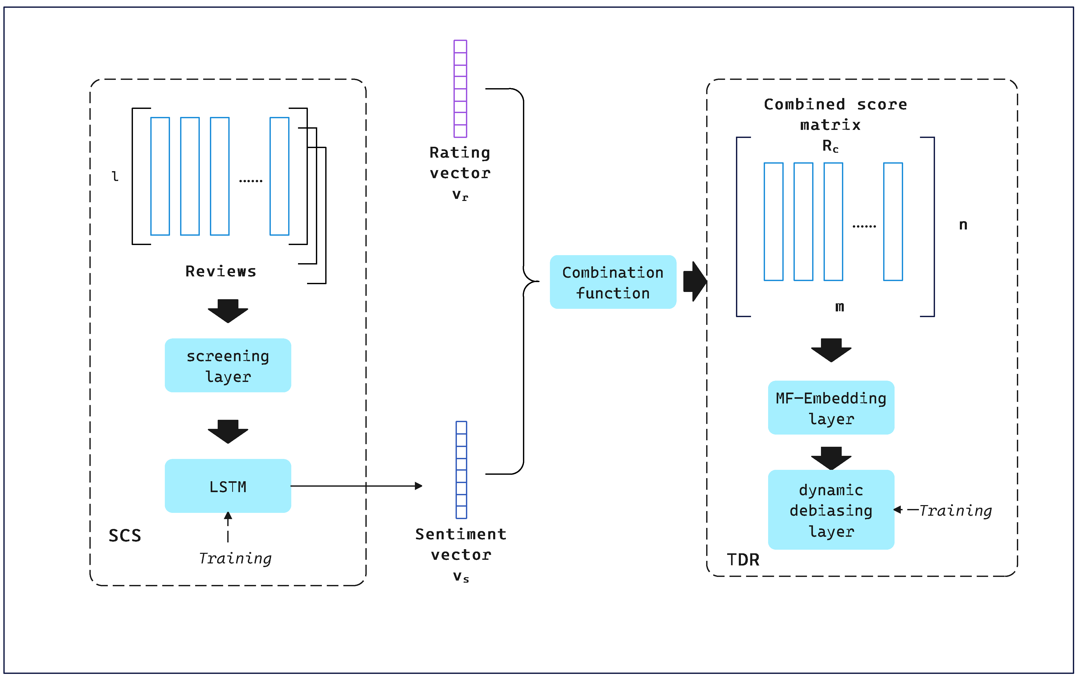
3.1. SCTD Framework
3.2. SCS
3.3. Combination Function
- Autofill: When the user u only rates or comments one item i, this time can cause gaps in the data and affect the accuracy of the combined function. To avoid this, ⊕ fills or .
- Selective Fill: If the user u has rated and commented on the item i, then a Drop judgment will be made first. If neither the user nor the item is deleted, ⊕ will be filled using a fixed weighted linear function .
- Drop: If , it is not processed. If , ⊕ decreases the user’s sentiment rating for item i. If , the same is not processed. If , ⊕ will remove user u. is the number of deleted comments. and ı are predefined thresholds.
3.4. TDR
4. Experiments
4.1. Datasets
4.2. Parameter Settings
4.3. Experimental Environment
4.4. Baselines
- (1)
- Static Average Item Rating (Avg): Avg is a simple recommendation method that calculates the average rating of each item based on historical user ratings.
- (2)
- Time-Aware Average Item Rating (T-Avg): T-Avg extends the traditional average item rating by incorporating temporal dynamics. It calculates item ratings based on recent user interactions, giving higher weight to more recent data.
- (3)
- Static Matrix Factorization (MF): This refers to a conventional matrix factorization model that presumes the selection bias remains constant over time.
- (4)
- Time-Aware Matrix Factorization (TMF) [17]: TMF is an advanced recommendation method that incorporates temporal dynamics into matrix factorization. It models how user preferences and item characteristics evolve over time by assigning time-dependent weights to user–item interactions.
- (5)
- MF-StaticIPS [5]: MF-StaticIPS is a recommendation system approach that combines matrix factorization (MF) with static inverse propensity scoring (Static IPS).
- (6)
- TMF-StaticIPS [32]: TMF-StaticIPS is a recommendation system approach that integrates temporal matrix factorization (TMF) with static inverse propensity scoring (Static IPS).
- (7)
- MF-DANCER [8]: MF-DANCER is a recommendation system method that combines matrix factorization removal and enhanced negative sampling. It corrects selection bias and addresses data sparsity by modeling bias and improving negative sampling.
- (8)
- TMF-DANCER [8]: TMF-DANCER extends MF-DANCER by incorporating temporal dynamics into matrix factorization.
- (9)
- Causal Intervention for Sentiment Debiasing (CISD) [33]: CISD aims to eliminate sentiment bias through causal inference. The model comprises two components: during the training phase, causal intervention is employed to block the influence of sentiment polarity on user and item representations, thereby reducing confounding effects; during the inference phase, adjusted sentiment information is introduced to enhance the personalization and accuracy of recommendations.
4.5. Evaluation Metrics
- (1)
- Mean-Squared Error (MSE): MSE measures the average squared difference between predicted and actual values, emphasizing larger errors and assessing model accuracy in regression tasks.
- (2)
- Mean Absolute Error (MAE): MAE is another metric for assessing regression models. Unlike MSE, MAE is less sensitive to outliers, providing a more robust measure of model accuracy.
- (3)
- Accuracy (ACC): It represents the proportion of correctly classified instances out of the total number of instances.
4.6. Experiment Results
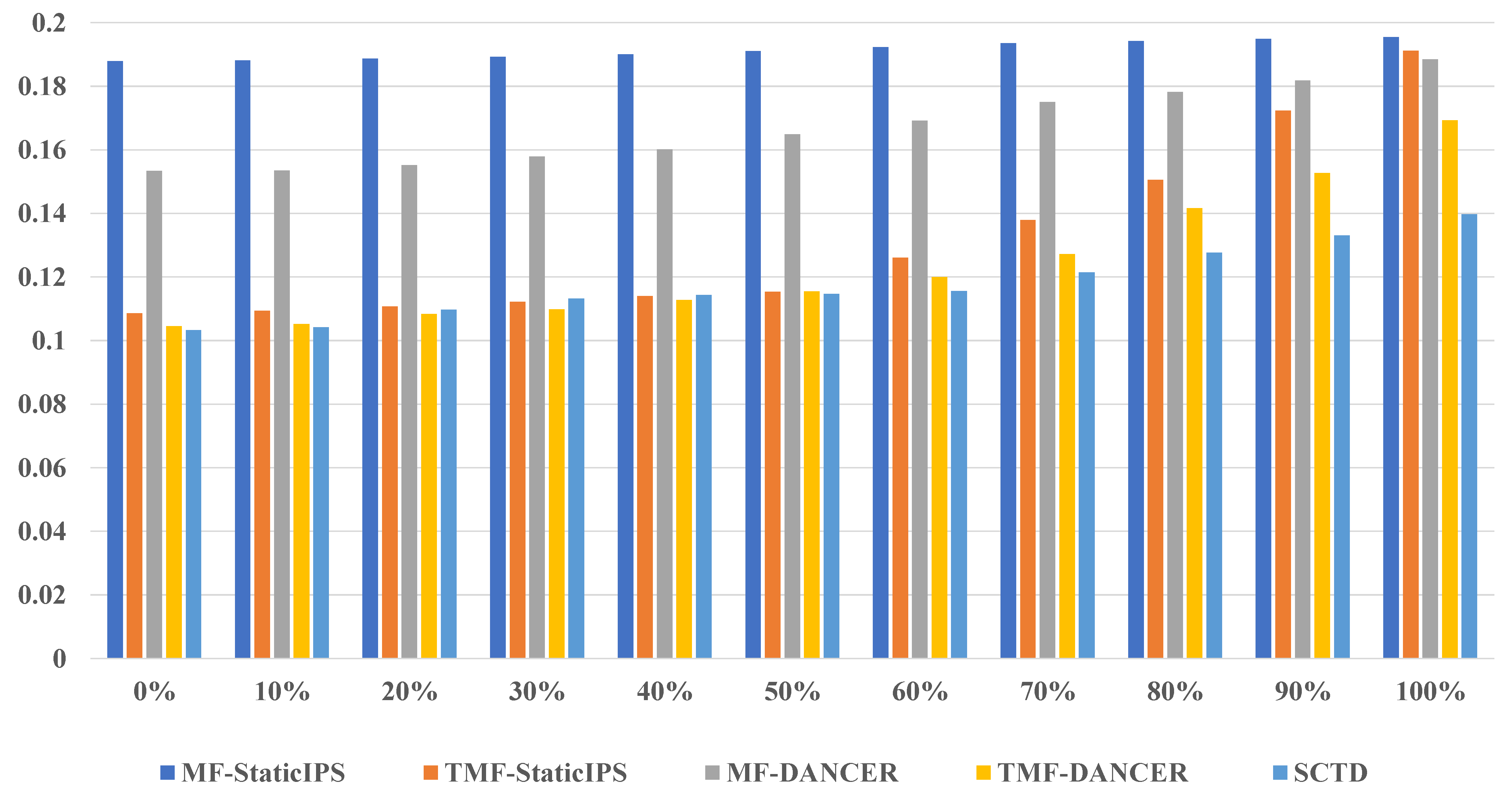
4.7. Parameter Analysis
5. Conclusions and Future Work
5.1. Conclusions
5.2. Future Work
Author Contributions
Funding
Institutional Review Board Statement
Informed Consent Statement
Data Availability Statement
Acknowledgments
Conflicts of Interest
Abbreviations
| IPS | Inverse Propensity Scoring |
| NLP | Natural Language Processing |
| MF | Matrix Factorization |
| CF | Collaborative Filtering |
| NCF | Neural Collaborative Filtering |
| AVG | Static Average Item Rating |
| SCTD | Sentiment Classification and Temporal Dynamic Debiased Recommendation Module |
| SCS | Sentiment Classification Scoring Module |
| TDR | Temporal Dynamic Debiased Recommendation Module |
| LSTM | Long Short-Term Memory |
References
- SIGIR ’24: Proceedings of the 47th International ACM SIGIR Conference on Research and Development in Information Retrieval; Association for Computing Machinery: New York, NY, USA, 2024.
- Marlin, B.M.; Zemel, R.S. Collaborative prediction and ranking with non-random missing data. In Proceedings of the Third ACM Conference on Recommender Systems, New York, NY, USA, 23–25 October 2009; pp. 5–12. [Google Scholar]
- Ovaisi, Z.; Ahsan, R.; Zhang, Y.; Vasilaky, K.; Zheleva, E. Correcting for selection bias in learning-to-rank systems. In Proceedings of the Web Conference 2020, Taipei, Taiwan, 20–24 April 2020; pp. 1863–1873. [Google Scholar]
- Pradel, B.; Usunier, N.; Gallinari, P. Ranking with non-random missing ratings: Influence of popularity and positivity on evaluation metrics. In Proceedings of the Sixth ACM Conference on Recommender Systems, Dublin, Ireland, 9–13 September 2012; pp. 147–154. [Google Scholar]
- Schnabel, T.; Swaminathan, A.; Singh, A.; Chandak, N.; Joachims, T. Recommendations as treatments: Debiasing learning and evaluation. In Proceedings of the International Conference on Machine Learning. PMLR, New York, NY, USA, 19–24 June 2016; pp. 1670–1679. [Google Scholar]
- Adamopoulos, P.; Tuzhilin, A. On over-specialization and concentration bias of recommendations: Probabilistic neighborhood selection in collaborative filtering systems. In Proceedings of the 8th ACM Conference on Recommender Systems, Silicon Valley, CA, USA, 6–10 October 2014; pp. 153–160. [Google Scholar]
- Li, H.; Zheng, C.; Wang, W.; Wang, H.; Feng, F.; Zhou, X.H. Debiased Recommendation with Noisy Feedback. In Proceedings of the 30th ACM SIGKDD Conference on Knowledge Discovery and Data Mining, New York, NY, USA, 25–29 August 2024; KDD ’24; pp. 1576–1586. [Google Scholar] [CrossRef]
- Huang, J.; Oosterhuis, H.; De Rijke, M. It is different when items are older: Debiasing recommendations when selection bias and user preferences are dynamic. In Proceedings of the Fifteenth ACM International Conference on Web Search and Data Mining, Virtual Event, 21–25 February 2022; pp. 381–389. [Google Scholar]
- Lin, A.; Wang, J.; Zhu, Z.; Caverlee, J. Quantifying and Mitigating Popularity Bias in Conversational Recommender Systems. In Proceedings of the 31st ACM International Conference on Information & Knowledge Management, New York, NY, USA, 17–21 October 2022; CIKM ’22; pp. 1238–1247. [Google Scholar] [CrossRef]
- Rubens, N.; Elahi, M.; Sugiyama, M.; Kaplan, D. Active learning in recommender systems. In Recommender Systems Handbook; Springer: Berlin/Heidelberg, Germany, 2015; pp. 809–846. [Google Scholar]
- Zhang, F.; Yuan, N.J.; Lian, D.; Xie, X.; Ma, W.Y. Collaborative knowledge base embedding for recommender systems. In Proceedings of the 22nd ACM SIGKDD International Conference on Knowledge Discovery and Data Mining, San Francisco, CA, USA, 13–17 August 2016; pp. 353–362. [Google Scholar]
- Panniello, U.; Tuzhilin, A.; Gorgoglione, M. Comparing context-aware recommender systems in terms of accuracy and diversity. User Model. User-Adapt. Interact. 2014, 24, 35–65. [Google Scholar] [CrossRef]
- Champiri, Z.D.; Shahamiri, S.R.; Salim, S.S.B. A systematic review of scholar context-aware recommender systems. Expert Syst. Appl. 2015, 42, 1743–1758. [Google Scholar] [CrossRef]
- Yang, X.; Guo, Y.; Liu, Y.; Steck, H. A survey of collaborative filtering based social recommender systems. Comput. Commun. 2014, 41, 1–10. [Google Scholar] [CrossRef]
- Beel, J.; Gipp, B.; Langer, S.; Breitinger, C. Paper recommender systems: A literature survey. Int. J. Digit. Libr. 2016, 17, 305–338. [Google Scholar] [CrossRef]
- Cai, Y.; Guo, J.; Fan, Y.; Ai, Q.; Zhang, R.; Cheng, X. Hard Negatives or False Negatives: Correcting Pooling Bias in Training Neural Ranking Models. In Proceedings of the 31st ACM International Conference on Information & Knowledge Management, Atlanta, GA, USA, 17–21 October 2022; CIKM ’22; pp. 118–127. [Google Scholar] [CrossRef]
- Koren, Y. Collaborative filtering with temporal dynamics. In Proceedings of the 15th ACM SIGKDD International Conference on Knowledge Discovery and Data Mining, Paris, France, 28 June–1 July 2009; pp. 447–456. [Google Scholar]
- Ren, Y.; Tang, H.; Zhu, S. Unbiased Learning to Rank with Biased Continuous Feedback. In Proceedings of the 31st ACM International Conference on Information & Knowledge Management, Atlanta, GA, USA, 17–21 October 2022; CIKM ’22; pp. 1716–1725. [Google Scholar] [CrossRef]
- Karatzoglou, A.; Hidasi, B. Deep Learning for Recommender Systems. In Proceedings of the Eleventh ACM Conference on Recommender Systems, Como, Italy, 27–31 August 2017; RecSys ’17; pp. 396–397. [Google Scholar] [CrossRef]
- Saelim, A.; Kijsirikul, B. A Deep Neural Networks model for Restaurant Recommendation systems in Thailand. In Proceedings of the 2022 14th International Conference on Machine Learning and Computing, Guangzhou, China, 18–21 February 2022; ICMLC ’22; pp. 103–109. [Google Scholar] [CrossRef]
- He, X.; Deng, K.; Wang, X.; Li, Y.; Zhang, Y.; Wang, M. LightGCN: Simplifying and Powering Graph Convolution Network for Recommendation. In Proceedings of the 43rd International ACM SIGIR Conference on Research and Development in Information Retrieval, Virtual Event, 25–30 July 2020; SIGIR ’20; pp. 639–648. [Google Scholar] [CrossRef]
- Xu, Y.; Yang, Y.; Han, J.; Wang, E.; Zhuang, F.; Yang, J.; Xiong, H. NeuO: Exploiting the sentimental bias between ratings and reviews with neural networks. Neural Netw. 2019, 111, 77–88. [Google Scholar] [CrossRef] [PubMed]
- Da, Y.; Bossa, M.N.; Berenguer, A.D.; Sahli, H. Reducing Bias in Sentiment Analysis Models Through Causal Mediation Analysis and Targeted Counterfactual Training. IEEE Access 2024, 12, 10120–10134. [Google Scholar] [CrossRef]
- Zhu, Y.; Yi, J.; Xie, J.; Chen, Z. Deep Causal Reasoning for Recommendations. ACM Trans. Intell. Syst. Technol. 2024, 15. [Google Scholar] [CrossRef]
- He, X.; He, Z.; Du, X.; Chua, T.S. Adversarial Personalized Ranking for Recommendation. In Proceedings of the The 41st International ACM SIGIR Conference on Research & Development in Information Retrieval, Ann Arbor, MI, USA, 8–12 July 2018; SIGIR ’18; pp. 355–364. [Google Scholar] [CrossRef]
- Wang, H.; Zhang, F.; Zhao, M.; Li, W.; Xie, X.; Guo, M. Multi-Task Feature Learning for Knowledge Graph Enhanced Recommendation. In Proceedings of the The World Wide Web Conference, San Francisco, CA, USA, 13–17 May 2019; WWW ’19; pp. 2000–2010. [Google Scholar] [CrossRef]
- Abusitta, A.; Li, M.Q.; Fung, B.C. Survey on Explainable AI: Techniques, challenges and open issues. Expert Syst. Appl. 2024, 255, 124710. [Google Scholar] [CrossRef]
- Koren, Y.; Rendle, S.; Bell, R. Advances in collaborative filtering. In Recommender Systems Handbook; Springer: Berlin/Heidelberg, Germany, 2021; pp. 91–142. [Google Scholar]
- Rosenthal, S.; Farra, N.; Nakov, P. SemEval-2017 task 4: Sentiment analysis in Twitter. arXiv 2019, arXiv:1912.00741. [Google Scholar]
- Han, J.; Zuo, W.; Liu, L.; Xu, Y.; Peng, T. Building text classifiers using positive, unlabeled and ‘outdated’examples. Concurr. Comput. Pract. Exp. 2016, 28, 3691–3706. [Google Scholar] [CrossRef]
- Liu, Q.; Wu, S.; Wang, L. Cot: Contextual operating tensor for context-aware recommender systems. In Proceedings of the AAAI Conference on Artificial Intelligence, Austin, TX, USA, 25–30 January 2015; Volume 29. [Google Scholar]
- Zhang, Y.; Yin, C.; Lu, Z.; Yan, D.; Qiu, M.; Tang, Q. Recurrent Tensor Factorization for time-aware service recommendation. Appl. Soft Comput. 2019, 85, 105762. [Google Scholar] [CrossRef]
- He, M.; Chen, X.; Hu, X.; Li, C. Causal Intervention for Sentiment De-biasing in Recommendation. In Proceedings of the 31st ACM International Conference on Information & Knowledge Management, Atlanta, GA, USA, 17–21 October 2022; CIKM ’22; pp. 4014–4018. [Google Scholar] [CrossRef]


| Dataset | Users | Items | Reviews | Ratings | Sparsity | Avg Words/s | Avg Words/r | Avg Sentences/r | Avg Reviews/u |
|---|---|---|---|---|---|---|---|---|---|
| Yelp | 45,980 | 11,537 | 229,900 | 229,900 | 0.043% | 9.9 | 130 | 11.9 | 5.00 |
| Jingdong | 8031 | 3025 | 8310 | 25,152 | 0.12% | 13.2 | 70 | 5.1 | 1.03 |
| Parameter | Value |
|---|---|
| CPU | 12vCPU Intel(R) Xeon(R) Platinum 8352V CPU @ 2.10 GHz |
| Memory | 90 GB |
| GPU | NVIDIA RTX 3090 (24 GB) |
| CUDA | 11.7 |
| Python | 3.10 |
| PyTorch | 1.12.1 + cu116 |
| Transformers | 4.21.3 |
| NLTK | 3.7 |
| Numpy | 1.22.4 |
| Method | MSE | MAE | ACC |
|---|---|---|---|
| Avg | 0.3155 | 0.4321 | 0.3623 |
| T-Avg | 0.328 | 0.4326 | 0.3614 |
| MF | 0.1811 | 0.3314 | 0.468 |
| TMF | 0.1338 | 0.2818 | 0.5396 |
| MF-StaticIPS | 0.1879 | 0.3377 | 0.4598 |
| TMF-StaticIPS | 0.1086 | 0.2491 | 0.6065 |
| MF-DANCER | 0.1533 | 0.3032 | 0.5074 |
| TMF-DANCER | 0.1045 | 0.2444 | 0.6151 |
| CISD | 0.1687 | 0.2958 | 0.5633 |
| SCTD | 0.1032 | 0.2527 | 0.6202 |
| Method | MSE | MAE | ACC |
|---|---|---|---|
| MF-StaticIPS | 0.1916 | 0.3428 | 0.4437 |
| TMF-StaticIPS | 0.1275 | 0.3124 | 0.5642 |
| MF-DANCER | 0.1629 | 0.2979 | 0.4926 |
| TMF-DANCER | 0.1178 | 0.2974 | 0.5831 |
| CISD | 0.1848 | 0.3326 | 0.5449 |
| SCTD | 0.1109 | 0.2831 | 0.5992 |
| Metric | SCTD Mean | TMF-DANCER Mean | Mean Difference | 95% Confidence Interval | p-Value |
|---|---|---|---|---|---|
| MSE | 0.1032 | 0.1045 | −0.0013 | [−0.0021, −0.0005] | 0.003 |
| MAE | 0.2527 | 0.2444 | +0.0083 | [−0.0001, +0.0167] | 0.052 |
| ACC | 0.6202 | 0.6151 | +0.0051 | [+0.0012, +0.0089] | 0.021 |
Disclaimer/Publisher’s Note: The statements, opinions and data contained in all publications are solely those of the individual author(s) and contributor(s) and not of MDPI and/or the editor(s). MDPI and/or the editor(s) disclaim responsibility for any injury to people or property resulting from any ideas, methods, instructions or products referred to in the content. |
© 2025 by the authors. Licensee MDPI, Basel, Switzerland. This article is an open access article distributed under the terms and conditions of the Creative Commons Attribution (CC BY) license (https://creativecommons.org/licenses/by/4.0/).
Share and Cite
Zhang, F.; Luo, W.; Yang, X. Mitigating Selection Bias in Recommendation Systems Through Sentiment Analysis and Dynamic Debiasing. Appl. Sci. 2025, 15, 4170. https://doi.org/10.3390/app15084170
Zhang F, Luo W, Yang X. Mitigating Selection Bias in Recommendation Systems Through Sentiment Analysis and Dynamic Debiasing. Applied Sciences. 2025; 15(8):4170. https://doi.org/10.3390/app15084170
Chicago/Turabian StyleZhang, Fan, Wenjie Luo, and Xiudan Yang. 2025. "Mitigating Selection Bias in Recommendation Systems Through Sentiment Analysis and Dynamic Debiasing" Applied Sciences 15, no. 8: 4170. https://doi.org/10.3390/app15084170
APA StyleZhang, F., Luo, W., & Yang, X. (2025). Mitigating Selection Bias in Recommendation Systems Through Sentiment Analysis and Dynamic Debiasing. Applied Sciences, 15(8), 4170. https://doi.org/10.3390/app15084170