An Integrated Optimization Method for Resource-Constrained Schedule Compression Under Uncertainty in Construction Projects

Abstract

An integrated solution that considers the shortening of scheduling and the planning of resource integration was conceived. The proposed method allocates the resources and the execution mode costs effectively in order to minimize the project duration and the cost of construction activities. Costs are managed based on the management of the costs already in place for people and those costs involved in the modes of execution of the project, trying to decrease the cost as much as possible. The proposed method is used in order to achieve the maximum potential and minimum costs during a project, including direct costs, indirect costs, and delay penalties. Furthermore, it finds a balance between the costs of acquiring and releasing human resources. The most interesting aspect of the proposed method is that it suggests addressing problems with resource planning and project scheduling simultaneously under uncertainty. FS theory is used to model project activity duration and cost uncertainty in the method. In addition, the above approach involves a genetic algorithm (GA) for schedule optimization. The optimization method utilizes a GA as an optimization approach to identify a set of non-dominated solutions. In this paper, we discuss how string-based multi-object optimization can be solved with ES using the elitist non-dominated sorting genetic algorithm (NSGA-II). The method is implemented in Python (v3.12.9), the computer programming language, as a standalone automated computational tool for schedule optimization in order to subsequently reschedule.

1. Introduction

Although significant efforts are ongoing in construction projects using project management methods to have them completed within their budgets and schedules, construction is characterized by delays and overrun costs. Delayed projects and over-run costs greater than 100% of the initially planned project duration and cost are common in developing countries, and, usually, the contractors and the project owners are in disagreement [1].

Schedule compression in the construction sector has received consideration as an initiative to address these challenges from the academic research and professional practice points of view. Both project owners and contractors gain benefits in reducing the project length for different reasons. Therefore, contractors speed up the completion of the project to fulfil contracted items, to avoid delays in the project, and use the least time possible to complete the projects. Project owners wants to speed up project delivery so that the project meets the needs of the market conditions and stakeholders. The time–cost problem, which what this process is known as in the academic literature, involves selecting the minimum cost duration so any project can be implemented with a given duration [2]. Thus, decreasing the project schedule duration leads to increases in the direct and decrements in the indirect costs. The expenses incurred for all resources utilized in the project execution phase form a part of the direct costs, and indirect costs and are spent even without the work being performed. Shortening the schedule necessitates hiring additional resources to accelerate individual activities, which gradually raises direct costs while steadily decreasing indirect costs. In view of this, academics and industry experts have been interested in the reduction in these supplementary direct expenses and the identification of the best minimum cost duration.

Resource planning, allocation, and leveling are major challenges for executing compressed construction projects. Researchers and industry experts have devised various techniques so that they can optimize scheduling and minimize the project duration at the minimum cost. The critical path method (CPM) has been one of the most used methods for scheduling in construction. CPM scheduling was introduced in the late 1950s by Morgan Walker and James Kelley to minimize the expenses resulting from the interruption and subsequent resumption of project operations when scheduling is not effective. CPM works very well in identifying the critical duration of a project and reducing the overall duration of a project. However, this is not a part of resource planning in the scheduling process, and substantial expenses as the result of disproportionately allocating a certain resource have been pointed out and called resource leveling [3]. In order to meet the continuous and variable demands for resources over time, the amendment of these resources to meet these needs requires additional cost, which includes the cost of hiring and termination, which is called acquisition and releasing.

In the problem of resource planning, contending with the uncertainty around activity duration and cost adds to the complexity, making this an inherently hard combinatorial problem. Project management is complex because it is based on the unrealistic expectation that project managers know the exact duration and cost of each activity in advance. In truth, construction projects are inherently unique, as no two projects are the same in any manner. Such uncertainty in project execution is influenced by the combined effects of many internal and external factors (e.g., economic and social pressure, work risks, and climatic changes). To deal with these uncertainties, a framework that can consider these factors properly is probability theory, which has been adopted by researchers dealing with this type of project. 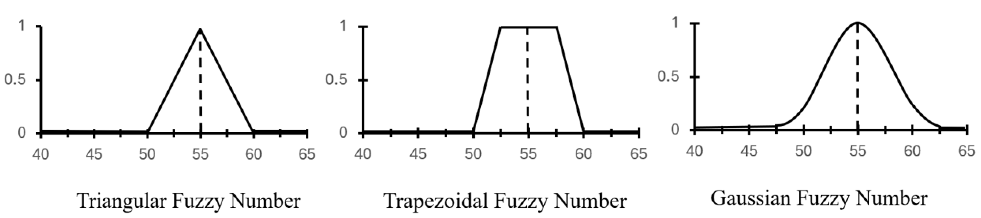It is difficult to store, record, and analyze historical construction data; thus, cost and time data are not easy to use and have not been frequently used to solve this problem in the past [4]. Therefore, the probabilistic distributions for different project activities cannot be accurately determined. To address the challenges mentioned above, FST, which analyzes uncertainty-related factors, is a more promising way. Unsurprisingly, the membership of an element in a fuzzy set is any real value between 0 and 1, and so, it is much more suitable for representing uncertainty if the numerical boundaries of element membership cannot be associated accurately. Once fuzzy models are properly used, then construction projects can be more accurately scheduled, such that, at the same time, we can achieve accuracy and efficiency in production planning.

The purpose of this research was to find a model for compressing construction schedules under resource constraints, while taking into account resource leveling as well as the uncertainty related to both the cost of the activity and its duration. In order to achieve this goal, there were subobjectives we fulfilled, which were

• Determining model uncertainties related to activity duration and cost.
• Optimizing resource allocation and leveling.
• Developing a fully automated and efficient computational tool.

By fulfilling these objectives, this study aimed to bridge the gaps in construction scheduling methodologies and provide a more effective framework for project acceleration while maintaining cost efficiency and resource optimization.

2. Literature Review

The available literature provides various approaches and algorithms for optimizing project scheduling by leveraging well-defined objective functions aligned with decision-makers’ goals. These methods aim to enhance the efficiency of planning for resource-limited projects and reduce project duration.

Exact, heuristic, and metaheuristic or evolutionary methods are some of these algorithms. Methods are used with these algorithms for finding the optimal solution, but they can be computationally expensive for large problems. Heuristic methods are suitable for complex problems due to their ability to give good (not optimal) solutions quickly. A set of more technologically advanced methodologies based on metaheuristic and evolutionary methods, which have been largely inspired by natural phenomena, have been refined, leading to the search for high-quality solutions within a reasonable time. For objective functions, time, and cost, or quality-based classification is performed. Mathematical models for establishing relationships between objective functions and problem constraints are exact methods to determine the optimal solution exactly. These methods use different optimization techniques like linear programming, which is used when the relation between variables is linear, to help improve problem-solving processes.

Dynamic programming is also used as it allows problems to be broken down into smaller subproblems whose solutions are combined to solve the overall problem, and this helps reduce computational complexity and tends to improve performance. On the other hand, these methods are being very accurate in solving optimal solutions, so they are very reasonable in solving complex problems that need exact and reliable results [5]. Rules are used for solving complex problems, which involve heuristic methods; that is, heuristic methods use rules in order to select good solutions and discard the ones that are unacceptable, quickly jumping to a near or an optimal solution. The most used technique is branch and bound, which divides the problem and excludes unpromising solutions systematically based on estimated bounds, which enhances search efficiency. However, it is an effective technique for solving the traveling salesperson problem )TSP), for which the boundedness and branching algorithms can be used, but no single algorithm is suitable for all problems because the appropriate strategy depends upon the type of problem [6].

Advanced approaches, typically called metaheuristic and evolutionary algorithms, are applied to find solutions for complex problems such as total cost optimization (TCO). Despite computational constraints, the strategies used for finding solutions that are high quality are heuristic. The methods include genetic algorithms (GAs), which are inspired by natural evolution by selection, crossover, and mutation; ant colony optimization (ACO), which imitates the behavior of ants when searching for food to improve search efficiency; and particle swarm optimization (PSO), which uses swarm intelligence to obtain a fast and efficient solution. On the contrary, while the GA relies on natural selection, ACO and PSO utilize collective knowledge to enhance the search for solutions. At the same time, these algorithms are very powerful tools for speeding up and facilitating the finding of solutions to complex optimization problems that most traditional methods struggle to deal with.

The research on resource-constrained project scheduling and schedule compression can be divided into four categories: time cost optimization models, deterministic scheduling, scheduling under uncertainty, and resource allocation models. The objectives of the TCO model are minimizing project duration while following budget constraints [7]. Schedules based on resource availability and deadlines are optimized in deterministic models [8]. These concepts are applied to scheduling under uncertainty, which is related to unpredictable project conditions. Equations that are NP-hard problems include resource allocation models for optimizing project duration and cost, to ensure project resource usage is balanced and sound.

Different approaches to tackling the time–cost in project scheduling have been developed by researchers. The multiple binary decision method (MBDM) was suggested to minimize project duration at the minimum cost, and Ref [9] sed fuzzy cost analysis and expert judgment to optimize schedule compression. Ref. [10] applied a convex hull method and genetic algorithms in order to obtain optimal solutions, while [11] proposed an adaptive weight method for improving the search for superior solutions. Ref. [12] used an ant colony optimization (ACO) algorithm to solve time–cost trade-off problems [13]. A particle swarm optimization (PSO) algorithm was proposed to achieve superior solution quality and computational efficiency for large-scale projects. Researchers [14] used TLBO with a modified adaptive weight method to find better Pareto front solutions than the previous metaheuristic methods used in construction engineering and project management.

The resource-constrained project scheduling problem (RCPSP) is a major challenge since its basic form assumes that each activity is executed within a single mode within a single processing time using one unit of a single renewable resource. The one-mode resource-constrained project scheduling problem has been extended to the, mode resource-constrained project scheduling problem (MMRCPSP) where activities can be accomplished in different execution modes with different durations and resource requirements [15]. Several methods have been proposed to solve the MMRCPSP. A branch-and-bound method, developed by [16], and a global optimization algorithm for balancing [17] have been applied to deal with the among time, cost, and quality in this problem. Heuristic approaches have also been developed to solve this problem with better efficiency, including the multi-pass priority approach with backward planning [18]. Metaheuristic algorithms have recently been used in optimization studies. CP was applied to optimize schedule compression by [19,20], who developed a two-phase genetic algorithm to deal with the time–cost trade-off as well. The proposed multi-objective model for both renewable and non-renewable resources to maximize the net present value and minimize project duration is based on the genetic algorithm and simulated annealing [21]. This idea was first proposed by [22], namely, a classification of renewable and non-renewable resources. Similarly, Ref. [23] proposed an ant colony optimization (ACO) algorithm to deal with resource constraints, and other authors [24] utilized linear programming to determine the best way to execute activities while releasing the resources in predetermined quantities at predetermined times. Finally, Ref. [25] examined the multi-project scheduling problem, proposing resource-sharing policies to minimize deviations between planned and actual project completion times.

Project scheduling success relies on the amount of accurate information that can be collected before project initiation. However, data availability is limited to the estimation of the duration, costs, and resource availability. Because of these problems, researchers have chosen to adopt fuzzy set (FS) theory instead of stochastic models. Mathematical and metaheuristic models have been adopted. Risk levels [26] were defined with time–cost optimization with the use of the α-cut method; Ref. [27] integrated scheduling and resource allocation under uncertainty. Ref. [28] applied the ant colony optimization (ACO) algorithm to facilitate the time–cost trade-off decision-making process. Later, these inefficiencies were reduced using metaheuristic models. To perform scheduling, Ref. [29] applied a particle swarm optimization algorithm operating with a genetic algorithm. At the same time, Ref. [30] created a comprehensive model based on repetitive scheduling, fuzzy set theory, and genetic algorithms to optimize cost, delays, and scheduling.

Distributing resources according to constraints and leveling is a very complex problem that falls under the category of resource allocation scheduling problems in project management. The numbers of resources, activities, and execution modes make it a complex problem. Genetic-algorithm-based models [31] and NSGA-II applications have been developed extensively for different multi-mode project scheduling and resource leveling problems [32]. Recent research emphasizes incorporating resource allocation into time buffering via robust scheduling methods, which aim to increase efficiency between cost and quality in dynamic project environments.

Through a comprehensive review of the literature on schedule compression and project scheduling, several observations (gaps) were identified, along with potential improvements that could enhance the efficiency and accuracy of project schedules.

Table 1. Capabilities and limitations of the latest and most relevant methods.

Reference	Optimization Method	Criteria
		Multi-Objective Optimization	Consider Cost	Activity Uncertainty	Resource-Constrained	Resource Leveling	Delay Penalty	Acquiring Resources and Releasing Costs
[33]	SA	✓	✓	✓	✓
[34]	BIP	✓			✓		✓
[35]	GA			✓	✓
[36]	NSGA	✓	✓	✓	✓		✓
[37]	MILP	✓	✓			✓		✓
[38]	MILP			✓	✓
[39]	NSGA-II	✓	✓	✓	✓
[40]	MINLP	✓	✓	✓	✓
[41]	GA	✓	✓		✓		✓
[42]	EA			✓	✓
[43]	MINLP	✓	✓	✓	✓
[44]	NSGA-II	✓	✓
[45]	ACO	✓	✓		✓	✓
[46]	DES		✓	✓	✓			✓
[47]	DES		✓	✓			✓
[48]	GA	✓	✓	✓	✓
[49]	NSGA-II	✓	✓	✓		✓
[50]	NSGA-II	✓	✓	✓	✓
[51]	PSO	✓	✓
[52]	NSGA-II	✓			✓
[53]	GA	✓	✓		✓		✓	✓
[54]	MILP	✓	✓	✓	✓			✓
[55]	ACO				✓
[56]	NSGA-II	✓	✓		✓		✓	✓
[57]	GA	✓	✓		✓
[58]	SA	✓		✓	✓	✓

NOTES: (MILP) mixed-integer linear programming, (ACO) ant colony optimization, (PSO) particle swarm optimization, (BIP) binary integer programming, (MAWA-TLBO) modified adaptive weight approach and teaching learning-based optimization, (NLP) nonlinear programming, (EA) evolutionary-based algorithm, (GA) genetic algorithm, (NSGA-II) elitist non-dominated sorting genetic algorithm, (MINLP) mixed-integer nonlinear programming, (SA) simulated annealing, (DES) discrete event simulation.

provides a summary of the capabilities and limitations of the methods found in the most recent and relevant references in this field.

The gaps identified in previous research can be summarized as follows:

• Resource scheduling methods that are unconstrained by available resources.
• Deterministic scheduling methods under resource constraints.
• Scheduling methods that ignore delay penalties.
• Scheduling methods that do not consider the additional costs associated with resource management, whether during resource acquisition (hiring) or release (firing).

To address these research gaps, this paper presents a comprehensive approach that advances project scheduling models and schedule compression methodologies. The proposed framework effectively balances project duration, cost, and resource constraints, making it more applicable to real-world scenarios. This approach enhances execution efficiency and reduces overall project costs, providing an innovative model that surpasses the traditional scheduling methods in this field.

3. Proposed Work Methodology

This paper presents a method of addressing the project scheduling problem when constrained by resources in an uncertain environment. It picks the best possible solution from an array of non-dominating ones. Additionally, the integration of fuzzy set (FS) theory with a genetic algorithm (GA) is proposed in order to determine the duration and cost of project activities under uncertainty (uncertainty modeling). Project managers’ expertise is leveraged to estimate the execution times for each project activity in terms of optimistic time, expected time, and pessimistic time. The time required for each activity to be completed is calculated using the α-cut concept. The method used to support and enhance the improvement process is shown in Figure 1.

3.1. Modeling Framework for Uncertainty and Defuzzification

This model represents uncertainty in activity costs and durations using fuzzy set (FS) theory, where fuzzy input data are transformed into exact values. This methodology consists of two main phases: fuzzification and defuzzification. Fuzzification refers to the process of converting numerical values into fuzzy values that reflect the degree of uncertainty, while defuzzification replaces the fuzzy variable with a precise numerical value, facilitating data analysis and decision making based on the available information. A fuzzy set is classified as a fuzzy number if it exhibits normalcy, convexity, and boundedness. Fuzzy numbers may be represented using triangles, which are defined by three values used in modeling when the estimate is clearer with uncertainty regarding the maximum values; a trapezoid is used for four values to provide high flexibility when dealing with unconfirmed data; and Gaussian forms, depending on natural distribution, are used when the gradual change in data is more realistic, as shown in Figure 2.

According to [59], the configuration of the fuzzy membership function has a minimal impact on the majority of fuzzy system applications. As such, to represent the uncertainty when implementing a project’s operations, we use triangular fuzzy numbers (TFNs) for simplicity and efficiency. The α-cut method works, as we can figure out fuzzy membership functions using each α cut that is associated with a confidence level α, as shown in Figure 3. The code we designed for the uncertainty modeling and defuzzification module utilizes functions from Python Skfuzzy, which we used for implementing fuzzy logic operations. These functions enable the modeling of uncertain data and the transformation of fuzzy values into precise values (defuzzification), thereby enhancing the accuracy and efficiency of the computational processing of ambiguous variables.

(The details can be obtained through the computational routines developed in Python 3.12.9, which are included in Supplementary S1).

The concept is based on fuzzy set (FS) theory, enabling users to enter activity costs and durations utilizing triangular fuzzy representations. The triangular fuzzy number is defined with three values (a₁, a₂, a₃) denoting the least (minimum), most probable (likely), and highest (maximum) values, respectively. The α-cut technique is used as a defuzzification tool, facilitating the calculation of project costs and duration according to the user-specified α-cut value, which indicates the acceptable amount of risk. This approach computes the average of the right and left border values (a1 and a3), which denote the lower and higher boundaries of the α-cut levels, yielding accurate results.

3.2. Project Scheduling Module

Users must provide the details for each task in the scheduling module, including short and typical durations, precedence relationships, resource needs, and associated expenditures. The critical path module is used in Python to identify the critical activities within a project schedule. To accelerate the execution of project activities, the necessary resources are accordingly allocated, as well as the Gantt chart, which anticipates changes in resource requirements for each phase of the project, is developed and updated. The scheduling module undertakes the following processes to formulate a feasible project plan after analyzing the user’s inputs to determine the total project duration:

• Based on their precedence relationships, it calculates each project activity both forward and backward to determine if it is critical or noncritical.
• The module determines the latest start and end times as well as the earliest start times for every activity.
• To optimize efficiency, a project schedule is created by scheduling both critical and noncritical tasks as early as feasible.
• The resources needed for every project task are determined.
• To guarantee resource optimization, nonessential tasks are distributed according to the resources that are available.
• Depending on the resources available, nonessential tasks are divided into smaller parts if needed.
• To ensure optimal resource utilization, the splitting method is used for noncritical activities when resource demand exceeds supply.

(A scheduling module sample code is provided in Supplementary S2).

3.3. Cost Computation Module

To calculate the total cost of the project, the project manager must input a variety of data, including the contract duration, indirect costs incurred per day during the project, costs associated with acquiring and releasing resources, penalties for exceeding the contractual timeline, and rewards for early completion. These data are integrated with the scheduling outcomes to calculate the overall project expenditure, considering the following components:

• The direct cost is the cost of implementing each and all project activities.
• Indirect costs may include employee salaries, protection, water, electricity, internet, etc., and are calculated by multiplying the amount of indirect cost per day by the project implementation period.
• Expenses associated with obtaining and releasing resources are calculated by multiplying the number of resources acquired or released in each project period by the respective cost rates. This represents the additional expenses related to obtaining and releasing human resources.
• The delay penalty is determined by multiplying the disparity between the contractual project length and the actual project duration by the applicable bonus or penalty rate.

3.4. Methods of Optimization

Optimization means searching for the best global solution using an objective function with a given (or predefined) range of search space by maximizing or minimizing its value [60]. In operation research, optimization is crucial in making educated decisions and solving project challenges that occur before and during the execution of a project. The main purpose of optimization is to minimize or maximize a predesigned objective function so as to ensure the best solution or collection of possible alternatives under the conditions [61]. For such problems, several advanced algorithms exist for obtaining the optimal solutions, which are widely used in optimization processes [62]. Among these are genetic algorithms (GAs), which are particularly effective tools for addressing complex optimization problems, including those involving multiple objectives. GA was chosen due to its extensive use and proven success in solving optimization challenges across various fields. First, the genetic algorithm encodes parental solutions as chromosomes to create the first population. The population structure of the genetic algorithm in the optimization technique is shown in Figure 4.

The main aim of the optimization technique used in this research was to enhance the balance between time and cost, presented as a multi-objective optimization problem. The approach aims to determine the optimal schedules that reduce both the total project duration and cost while promoting the effective use of available resources. The elitist non-dominated sorting genetic algorithm (NSGA-II) was utilized for multi-objective optimization and searching for optimal non-dominated solutions due to its effectiveness in handling all possible solutions and obtaining optimal solutions in each simulation run based on the Pareto concept. NSGA-II was selected from among the multi-objective evolutionary optimization algorithms (MOEAs) because it has been widely used in numerous applications and is known for its reliability [63]. The algorithm utilizes a crossover operator to exchange genes between parent chromosomes and a mutation operator to introduce genetic diversity. In the developed methodology, the partial mapped crossover (PMX) is used to maintain the order of elements during crossover, while the simple reciprocal mutation operator swaps genes randomly.

3.4.1. Optimization Problem with Resource Constraints

Our method addresses the challenges due to restricted resources by adjusting the scheduling of noncritical activities within their allowable windows. The pseudocode below illustrates the programming logic used to solve this optimization problem.

Initialize the following parameters:

• Define project activities, duration, cost, and resources.
• Set constraints: resource limits, project deadline, precedence relationships.
• Initialize penalty factor δ and fitness value.

Define the following objective functions:

• Minimize project duration: T = sum (X_jm ∗ T_jm) for all j in CA.
• Minimize project cost: C = sum ([AC_R ∗ sum(I_tr) + RC_r ∗ sum(D_tr)] + sum (X_jm ∗ C_jm) + IC ∗ T + (T−G) ∗ P)

Check the following constraints:

• Duration constraint: ensure noncritical activity durations match execution mode.
• Network constraint: maintain precedence relations among activities.
• Resource constraint: ensure total resource demand does not exceed available resources.

Apply penalty function.

• Compute penalty = δ(C_max) ∗ max ((max.daily consumption/resource level)−1, 0)
• Adjust fitness value: fitness = C_max + penalty.

Generate initial schedule.

• Assign execution modes to each activity.
• Compute earliest start and finish times for all activities.

Optimization loop.

• Evaluate schedule feasibility.
• Adjust noncritical activities within floating periods to balance resource demands.
• If infeasible, increase penalty δ.
• If feasible, update the best solution.

Decision support.

• Compute weighted sum for Pareto-optimal solutions.
• Select optimal solution using normalized objective functions.

Output final optimized schedule and cost.

When the resource demand exceeds availability, noncrucial activities are redistributed inside their floating intervals to balance the resource allocation. The steps for generating an optimal project schedule and cost estimation using optimization techniques are presented in the flowchart shown in Figure 5.

Additionally, a penalty function is used to deal with instances where resource demand surpasses availability. Several penalty functions are proposed in the literature, with one of the most useful being the death penalty, which, without delay, removes any infeasible answer. The penalty function we implemented is mathematically defined using Equation (1).

$$\mathit{Penalty}=\delta \left(C_{max}\right). max ({\displaystyle \frac{max. daily consumption }{resurce level}}-1.0)$$

(1)

where δ represents the fitness factor of the modern solution, which is more than one; C_max denotes fitness value of the current solution before the penalty is applied. Consequently, Equation (2) offers the correct definition of the fitness function for infeasible solutions.

$$\mathrm{Fitness} \mathrm{value}={\mathrm{C}}_{\max } + \mathrm{penalty}$$

(2)

Increasing the penalty fee δ effectively transforms the penalty into a “death penalty”, thereby preventing the current solution from advancing to the next era. Conversely, decreasing δ leads to the current solution advancing to the next era. Thus, it is critical to find a balance: the goal is to dispose of infeasible solutions to achieve the optimal solution while preventing stagnation in local optima through maintaining variability. A penalty cost of 0 suggests that the current answer is possible.

3.4.2. Objective Function

The primary goals of this method is to obtain a project schedule with the lowest possible duration and direct cost. When the project duration is reduced, indirect costs are reducing while ensuring the availability of resources for all project activities. The objective functions are presented in Equations (3) and (4).

$$\mathrm{Minimize} \mathrm{T}={{\displaystyle \sum }}_{m=1}^{M_j}{X}_{jm}{T}_{jm} {\sum }_{j=1}^{CA}$$

(3)

where CA is critical activity, $M_j$ is the number execution modes for an activity, $T_{jm}$ is duration j in mode m; m = 1, 2 … $M_j$; $X_{jm}a$ binary variable that takes a value of 1 if activity j is carried out according to mode M and takes a value of 0 otherwise.

$$\mathrm{Minimize} C = {{\displaystyle \sum }}_{r=1}^R[A{C}_R{{\displaystyle \sum }}_{t=1}^T{I}_{tr}+R{C}_r{{\displaystyle \sum }}_{t=1}^T{D}_{tr}]+{{\displaystyle \sum }}_{m=1}^{M_j}\left[X_{jm}{C}_{jm}\right]+IC T+\left[\left(T-G\right)P\right]$$

(4)

where C is the cost of the project, R is the number of resources in the project, $A{C}_R$ is the cost of acquiring the resource, T is the project duration; t is time; t is $E{S}_j$ to $L{F}_j$; $I_{tr}$ is the amount of resource r acquired during time t; $R{C}_r$ is the release cost of resource r; $D_{tr}$ is the resource r released during time t; $C_{jm}$ is the direct cost of activity j in mode m; IC is indirect cost; G is the contracted project duration; P is the delay penalty.

3.4.3. Problem Constraints

The constraints (duration constraints, resource constraints, and project network constraints) are expressed mathematically using the following equations:

The duration constraint defines the total active durations for a noncritical activity (j), which must match its duration $D_{jm}$ when executed in mode m, as outlined in Equation (5).

$${{\displaystyle \sum }}_{\mathrm{t}={\mathrm{ES}}_{\mathrm{j}}}^{{\mathrm{LF}}_{\mathrm{j}}}{\mathrm{k}}_{\mathrm{tj}}={{\displaystyle \sum }}_{\mathrm{m}=1}^{{\mathrm{M}}_{\mathrm{j}}}{\mathrm{D}}_{\mathrm{jm}}{\mathrm{X}}_{\mathrm{jm}}; \mathrm{j}=1, \dots , \mathrm{nn}$$

(5)

where ${\mathrm{k}}_{\mathrm{tj}}$ is a binary variable for project duration, which equals 1 when j is progressing on time t; t is ${\mathrm{ES}}_{\mathrm{j}}$ to ${\mathrm{LF}}_{\mathrm{j}}$; ${\mathrm{M}}_{\mathrm{j}}$ is the mode of executing activity j, j = 1, 2, … N; ${\mathrm{D}}_{\mathrm{jm}}$ is the duration of activity j in mode m, m = 1, 2, … ${\mathrm{M}}_{\mathrm{j}}$.

The network constraint guarantees the preservation of the preceding connections for activities. Identifying the mode for each action is critical for defining these restrictions. Mathematically, Equation (6) states that each activity can operate in only one mode.

$${{\displaystyle \sum }}_{\mathrm{m}=1}^{{\mathrm{M}}_{\mathrm{j}}}{\mathrm{X}}_{\mathrm{jm}}=1; \mathrm{j} = 1, \dots , \mathrm{N}$$

(6)

To calculate the start and end times of all activities, Equations (7) and (8) are utilized.

$${\mathrm{S}}_{\mathrm{j}}=\left(\mathrm{T}+1\right)-\max \{\left(\mathrm{T}+1-\mathrm{t}\right){\mathrm{k}}_{\mathrm{tj}};\mathrm{t}={\mathrm{ES}}_{\mathrm{j}},{ \mathrm{ES}}_{\mathrm{j}}+{\mathrm{TF}}_{\mathrm{j}}$$

(7)

$${\mathrm{F}}_{\mathrm{j}}=\max ({\mathrm{t} \mathrm{k}}_{\mathrm{tj}};\mathrm{t}={\mathrm{LF}}_{\mathrm{j}}-{\mathrm{TF}}_{\mathrm{j}}, {\mathrm{LF}}_{\mathrm{j}})$$

(8)

where S_j is the start time of activity j; $F_j$ is the finish time of activity j. The logical network constraint is derived from the above equations and is expressed in Equation (9).

$${\mathrm{l}}_{\mathrm{c}}\ge {\mathrm{F}}_{\mathrm{j}}+1 \mathrm{when} \mathrm{j}=1, \dots ,\mathrm{N} \mathrm{k}\in \mathrm{succession} \mathrm{j}$$

(9)

The resource constraint guarantees that the aggregate demand for resource p in period t, in conjunction with the quantity of that resource released during the same period, which is the resource demand from period t − 1 plus the resources obtained at time t. To define the constraint, the resource requirement (${\mathrm{RR}}_{\mathrm{tp}}$) must first be expressed as a function of binary variables ${\mathrm{k}}_{\mathrm{ti}}$ and ${\mathrm{x}}_{\mathrm{jm}}$. In simpler terms, the requirement for resources at time (t) represents the total of the resources needed by all active activities at that time, as represented in Equation (10).

$${\mathrm{RR}}_{\mathrm{tr}}={{\displaystyle \sum }}_{\mathrm{j}=1}^{\mathrm{N}}{\mathrm{k}}_{\mathrm{tj}}{{\displaystyle \sum }}_{\mathrm{m}=1}^{{\mathrm{M}}_{\mathrm{j}}}{\mathrm{r}}_{\mathrm{jm}}{\mathrm{x}}_{\mathrm{jm}};\mathrm{t}=1, \dots , \mathrm{T}$$

(10)

3.5. Module for Decision Support

Multi-criteria selection methods enable the evaluation of a set of different criteria, facilitating the ranking of available alternatives and identifying the most suitable option based on specific requirements. In this method, the decision support module is implemented using the weighted sum method (WSM) to assist project managers in selecting the most appropriate scenario. This is achieved by generating 2D Pareto fronts for time and cost based on α-cut values and detailed project parameters, which facilitate the identification of the optimal solution. The weighted sum method (WSM) primarily relies on computing a preference index for each alternative, where the alternative with the lowest preference index is selected in minimization cases. The preference index is calculated using Equation (11).

$${\mathrm{p}}_{\mathrm{i}}={{\displaystyle \sum }}_{\mathrm{j}=1}^{\mathrm{n}}{\mathrm{v}}_{\mathrm{ij}}\times { \mathrm{w}}_{\mathrm{j}}$$

(11)

where ${\mathrm{p}}_{\mathrm{i}}$ represents the preference value of an alternative, ${\mathrm{v}}_{\mathrm{ij}}$ indicates the normalized performance metric, and ${\mathrm{w}}_{\mathrm{j}}$ signifies the weight assigned to each criterion. The variables m and n represent the number of criteria and alternatives Thus, the normalized objective function for the optimization approach is defined in Equation (12).

$$\mathrm{Normalized} \mathrm{Objective} \mathrm{function}=({\displaystyle \frac{\mathrm{duration} \ast \mathrm{weight}}{\mathrm{Sum} \mathrm{of} \mathrm{durations}}})+\left({\displaystyle \frac{\cos \mathrm{t} \ast \mathrm{weight}}{\mathrm{Sum} \mathrm{of} \cos \mathrm{ts}}}\right)$$

(12)

4. Model Implementation

4.1. Background

In this study, the methodology that was developed was then validated using a project case study in Babil Governorate, Iraq. The network of the project is shown in Figure 6, which depicts activities as letters (A—excavation, B—foundation, C—brick construction, D—exterior plumbing, E—electrical works, F—roofing, G—interior installation, H—cement wall coating, I—interior painting, J—flooring, K—external wall construction, L—exterior painting, M—interior fixtures, and N—exterior fixtures). The critical activities in the project were A, B, C, D, G, H, I, and M. Each activity had five execution modes to choose from, as indicated in

Table 2. Activity execution modes (durations).

Duration (Optimistic, Most Likely, Pessimistic) (Days)
Activity	Mode 1	Mode 2	Mode 3	Mode 4	Mode 5
A	(8, 9, 10)	(11, 12, 13)	(15, 16, 17)	(18, 19, 20)	(21, 22, 23)
B	(41, 42, 43)	(44, 45, 46)	(48, 49, 50)	(52, 53, 54)	(56, 57, 60)
C	(24, 26, 28)	(27, 29, 31)	(28, 30, 32)	(31, 33, 35)	(34, 36, 38)
D	(40, 41, 42)	(44, 45, 46)	(48, 49, 50)	(51, 52, 53)	(55, 56, 58)
E	(20, 22, 24)	(21, 23, 25)	(23, 25, 27)	(26, 28, 30)	(29, 31, 33)
F	(16, 18, 20)	(17, 19, 20)	(21, 22, 23)	(24, 25, 27)	(26, 28, 29)
G	(22, 24, 26)	(25, 27, 28)	(30, 32, 34)	(33, 35, 37)	(38, 39, 41)
H	(22, 23, 24)	(20, 21, 23)	(22, 24, 26)	(25, 27, 29)	(28, 30, 32)
I	(27, 29, 31)	(30, 32, 34)	(33, 35, 37)	(34, 36, 37)	(36, 38, 41)
J	(20, 22, 24)	(23, 25, 27)	(25, 27, 29)	(28, 30, 32)	(31, 33, 35)
K	(18, 19, 21)	(19, 21, 23)	(20, 22, 24)	(23, 25, 27)	(26, 28, 30)
L	(14, 16, 18)	(20, 22, 24)	(25, 27, 29)	(28, 30, 32)	(31, 33, 35)
M	(14, 16, 18)	(20, 22, 24)	(21, 23, 25)	(22, 24, 26)	(25, 27, 29)
N	(17, 18, 20)	(19, 21, 23)	(22, 24, 26)	(25, 27, 28)	(30, 32, 33)

and

Table 3. Activity execution modes (costs).

Direct Cost (Optimistic, Most Likely, Pessimistic) (USD 1000)
Activity	Mode 1	Mode 2	Mode 3	Mode 4	Mode 5
A	(14, 15, 17)	(11, 12, 13)	(8, 9, 10)	(5, 6, 7)	(2, 3, 4)
B	(97, 98, 100)	(93, 94, 96)	(89, 90, 92)	(85, 86, 88)	(81, 82, 84)
C	(39, 41, 42)	(38, 39, 40)	(34, 36, 37)	(32, 33, 35)	(29, 30, 31)
D	(86, 88, 90)	(85, 86, 87)	(82, 83, 84)	(78, 79, 80)	(74, 75, 76)
E	(30, 31, 33)	(27, 28, 29)	(24, 25, 26)	(20, 22, 23)	(17, 18, 19)
F	(33, 35, 38)	(30, 31, 33)	(27, 28, 29)	(24, 25, 26)	(18, 20, 22)
G	(32, 34, 36)	(30, 31, 33)	(27, 28, 29)	(22, 23, 25)	(16, 18, 20)
H	(38, 40, 42)	(37, 38, 39)	(32, 34, 36)	(27, 29, 30)	(22, 23, 25)
I	(42, 44, 46)	(39, 40, 41)	(35, 36, 38)	(30, 32, 33)	(24, 26, 28)
J	(40, 42, 46)	(35, 36, 38)	(32, 33, 35)	(26, 28, 30)	(20, 21, 24)
K	(29, 30, 32)	(25, 26, 28)	(21, 22, 23)	(15, 17, 19)	(8, 10, 12)
L	(28, 30, 35)	(26, 28, 30)	(22, 24, 25)	(16, 18, 19)	(17, 15, 14)
M	(17, 18, 21)	(13, 15, 16)	(10, 11, 12)	(7, 8, 9)	(4, 5, 6)
N	(18, 20, 22)	(14, 16, 17)	(11, 12, 13)	(8, 9, 10)	(5, 6, 7)

. The time and cost of each option are represented using triangular fuzzy numbers. The first and third correspond to the maximum and minimum values, respectively, for time and cost, and the second is the most probable estimate for both parameters. In order to choose the best alternatives from a set of non-dominant solutions, the SUM is used as a decision-making tool to identify the optimal time–cost solution. We evaluate the capability and efficiency of the NSGA-II method developed in this research by comparing the obtained results with those of the actual project.

The following modifications were implemented in the case study to address the problem in a resource-constrained environment:

• The resources required for each activity were computed using Equation (13) and are shown in

  Table 4. Implementation modes for each activity (resources).

  Activity	A	B	C	D	E	F	G	H	I	J	K	L	M	N
  Mode 1	7	9	6	9	6	8	6	7	6	8	6	8	5	4
  Mode 2	4	8	6	8	5	7	6	7	5	6	5	5	3	3
  Mode 3	2	7	5	7	4	5	4	6	4	5	4	4	2	2
  Mode 4	1	7	4	6	3	4	3	4	4	4	3	2	1	1
  Mode 5	1	6	3	5	2	3	2	3	3	3	1	2	1	1

  , with the resource cost approximated at USD 250 per day.
• The project parameters listed in

  Table 5. Parameters of project.

  Indirect cost (USD)	300
  Direct cost	575,000
  Contractual duration (day)	285
  Acquiring costs (USD)	250
  Releasing costs (USD)	250
  Delay penalty (USD/day)	500
  Available resources (day)	9
  Alpha cut	0.5

  were used, with the costs of releasing and acquiring estimated based on project manager experience and prevailing market prices.

Required resources = (cost of activity)/(duration activity × USD 250 per day)

(13)

4.2. Sensitivity Analysis of the Genetic Algorithm

The quality of the optimization solution obtained with a GA may be affected by the algorithm’s parameters, including population size, mutation rate, and crossover rate. Typically, these parameters are selected by the user without clear guidelines on the optimal values that yield the best solution. Therefore, sensitivity analysis procedures are implemented depending on the case to determine the effect of the values on different parameters, including crossover probabilities (ranging from 0.4 to 1 in 0.2 increments), mutation probabilities (ranging from 0.2 to 0.8 in 0.2 increments), and population sizes (30, 50, and 60). These parameters are iteratively adjusted to assess their effect on solution quality. The following genetic algorithm parameters were adopted in the NSGA-II method based on the results of the sensitivity analysis:

• Population size = 50.
• Number of generations = 200.
• Mutation rate = 0.4.
• Crossover rate = 0.4”.

(The full sensitivity analysis is provided in the Supplementary S3).

5. Results of NSGA-II Optimization Approach

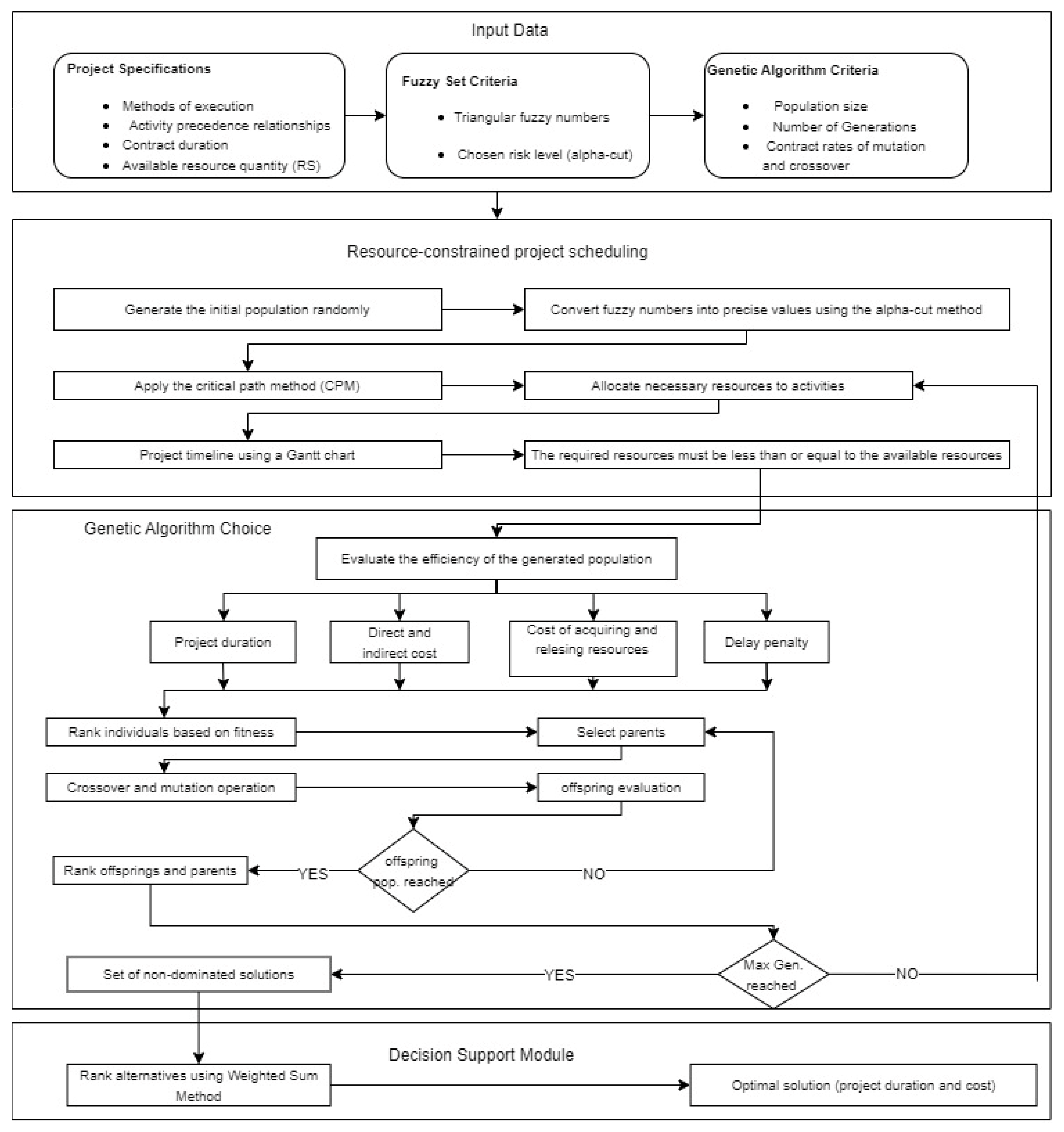
As shown in

Table 6. Set of solutions generated by NSGA-II.

Duration (Days)	Cost (USD)	Normalized Duration	Normalized Cost	(PI)
294	539,000	0.17324691	0.16447971	0.16886332
288	542,000	0.16971126	0.16539518	0.16805322
285	545,000	0.16794343	0.16631065	0.16712704
280	548,000	0.16499705	0.16722612	0.16611158
274	555,000	0.16263995	0.16783644	0.16523820
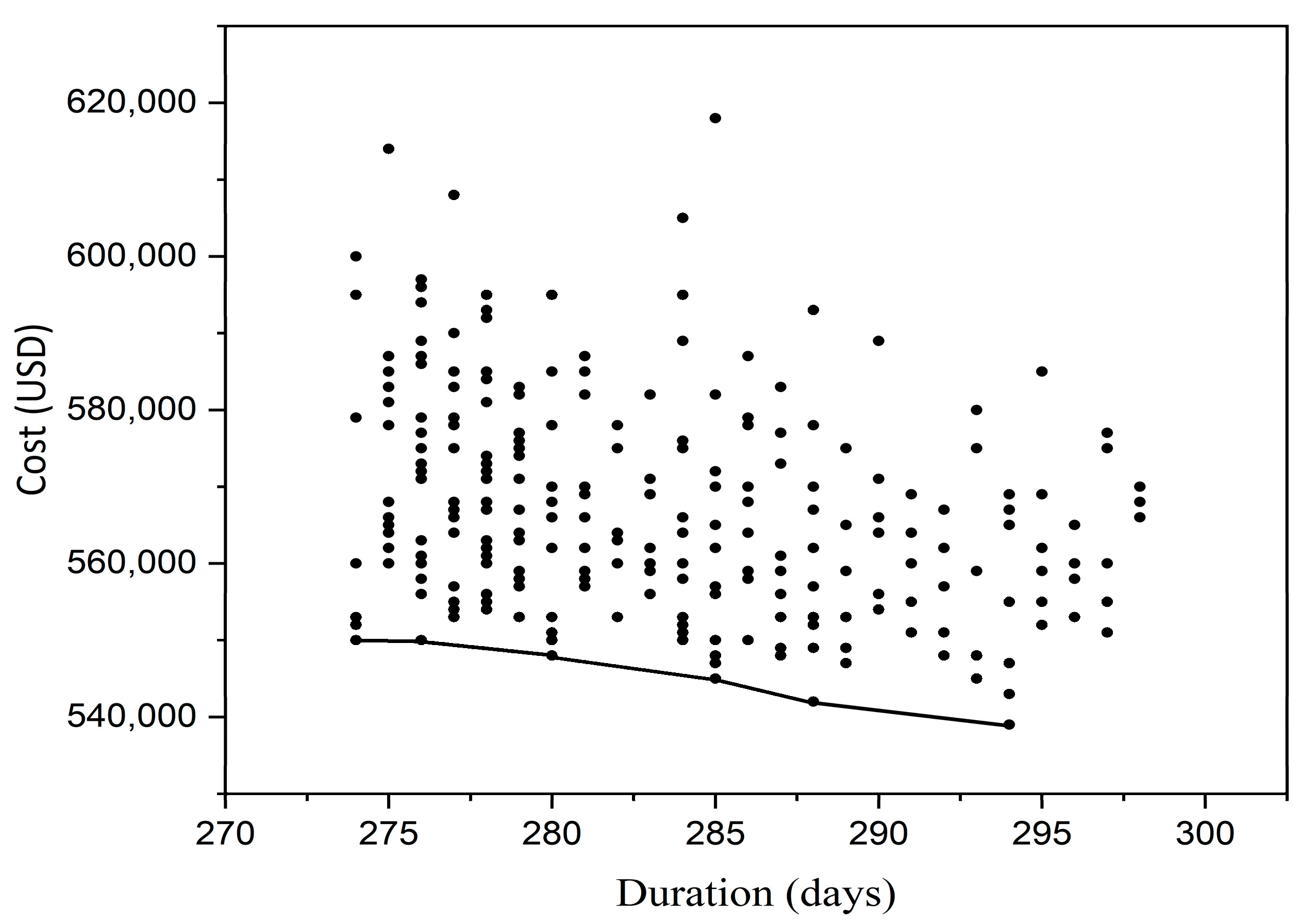
276	553,000	0.16146140	0.16875191	0.16510666

, the non-dominated set of solutions was generated after executing 200 generations in an optimized NSGA-II with population size = 50, crossover rate = 0.4, and mutation rate = 0.6. The optimal solution among them was identified using the weighted sum technique. The optimal choice was determined as the solution with the smallest preference index (PI), since the problem was solved using the minimization approach. The penultimate solution was the optimum, i.e., the PI value was 0.16549756, duration of implementation was 274 days and cost was USD 550,000. The solutions obtained after executing 200 generations using the optimization algorithm are presented in Figure 7. The curve illustrates the relationship between cost and time, representing the non-dominated set of solutions that reflects the best achievable balance between these two factors. This set comprises the most efficient solutions, where no single criterion can be improved without compromising the other.

Table 7. Assigned execution mode for each project activity (NSGA-II).

Activity	A	B	C	D	E	F	G	H	I	J	K	L	M	N
Mode 1	✗	✗	✗	✗	✗	✗	✗	✗	✗	✗	✗	✓	✓	✗
Mode 2	✗	✗	✗	✓	✗	✗	✗	✗	✗	✗	✓	✗	✗	✗
Mode 3	✓	✗	✗	✗	✓	✗	✗	✗	✗	✗	✗	✗	✗	✓
Mode 4	✗	✗	✗	✗	✗	✓	✗	✗	✓	✓	✗	✗	✗	✗
Mode 5	✗	✓	✓	✗	✗	✗	✓	✓	✗	✗	✗	✗	✗	✗

Note: A checkmark indicates the selected mode for the activity, while a cross represents an available mode that was not chosen.

represents the appropriate implementation mode for each of the activities in the project; it illustrates the execution mode for each project activity after applying the optimal solution identified through the optimization algorithm. This selection was made by achieving the optimal balance between cost, time, and resources based on the optimization criteria adopted in this study.

Based on Table 6, the selected execution mode for each project activity was determined.

Table 8. Optimal solution for project activities (time, cost, and resources).

Activities	A	B	C	D	E	F	G	H	I	J	K	L	M	N
Time/day	16	57	36	45	25	25	39	30	36	30	21	16	15	25
Cost/USD 1000	9	82	30	86	25	25	18	23	32	28	26	30	18	12
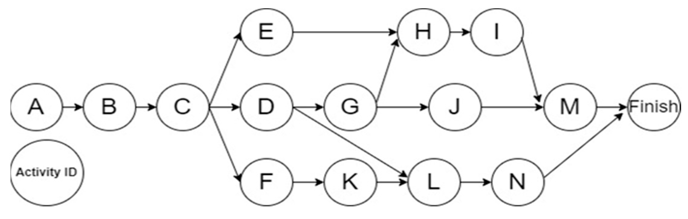
Resource (machine)	2	6	3	8	4	4	2	3	4	4	5	8	5	2

presents the optimal duration, cost, and resource allocation for each project activity. Furthermore, Figure 8 presents the project network, illustrating the execution time for each activity, the earliest start and finish times, the latest start and finish times, as well as the floating period duration.

The project cost distribution for the project using the method proposed in this study is presented in

Table 9. Distribution of project costs.

Project cost	USD 632,200
Direct cost	USD 550,000
Indirect cost	USD 82,200
Delay penalty	USD 0

. By comparing the obtained results (274 days and USD 632,200) with the contracted project duration and cost (285 days and USD 660,500), it is obvious that applying the method will lead to the project being completed in shorter time and at a lesser cost. We found that the proposed method is capable of finding a globally optimal solution and avoid entrapment in local minima. And, the main advantage of the method used for scheduling optimization is the implementation of the NSGA-II algorithm and its capability of reassigning resources for noncritical activities within their floating periods. This results in effective monitoring of constraints to resource without exceeding cost or duration of project activities.

Summary of Results

The optimization approach using the NSGA-II algorithm successfully identified an optimal project schedule by balancing cost, time, and resource constraints. After 200 generations, the best solution was determined using the weighted sum technique, with an optimal preference index (PI) of 0.16549756, a project duration of 274 days, and a total direct cost of USD 550,000. The analysis of the non-dominated set of solutions demonstrates that no single criterion (cost or time) could be improved without negatively impacting the other. By applying the optimal execution mode for each project activity (as detailed in Table 7 and Table 8), resources for noncritical activities within their floating periods are redistributed effectively using our method. Comparing the obtained results (274 days and USD 632,200) with the contracted project duration and cost (285 days and USD 660,500), using the proposed method achieved a shorter project duration and lower cost. This confirms the effectiveness of NSGA-II in avoiding local minima and identifying a globally optimal solution. The method’s ability to dynamically allocate resources while maintaining project constraints ensures an efficient and feasible scheduling solution.

6. Conclusions

Under resource constraints and uncertainty, this paper presents an integrated approach for shortening project schedules by combining resource planning scheduling with project scheduling. This approach was implemented within a computational framework based on Python. The method iteratively reschedules all project activities to achieve more efficient and optimized project scheduling. Based on the results obtained with NSGA-II, it is evident that the approach achieves a global optimal solution, effectively avoiding entrapment in local minima. This method assists both contractors and project managers in shortening the project schedule while ensuring the integrated and efficient utilization of resources. Moreover, the applied approach provides multi-objective improvements, particularly in scenarios characterized by uncertainty. It serves as a valuable tool for facilitating resource management and achieving a balance between cost and time. This enables contractors and project managers to select the optimal solution from the available alternatives, considering the specific conditions and challenges that may arise during project execution. The following are the weaknesses of the application mode:

• The use of fuzzy triangle numbers is limited to the modeling of uncertainty related to specific factors only.
• Linear developments, including the installation of electricity lines and pipes, are not considered.
• The scheduling of multiple constrained resources is overlooked.

Future directions for developing this method may include

• Expanding the scope of application to encompass linear projects, making the method more suitable for sectors such as energy and infrastructure.
• Incorporating additional membership functions beyond the triangular function, such as Gaussian or trapezoidal functions, to enhance the accuracy of uncertainty representation.
• Developing models that account for the multiple-resource-constrained scheduling problem, enabling more efficient project management.
• Exploring additional metaheuristic algorithms, such as harmony search or ant colony optimization, alongside the currently used genetic algorithm, to improve the method’s performance and optimization accuracy.

References

1. Memon, A.H.; Rahman, I.A.; Abdullah, M.R.; Asmi, A.; Azis, A. Factors Affecting Construction Cost in Mara Large Construction Project: Perspective of Project Management Consultant. Int. J. Sustain. Constr. Eng. Technol. 2010, 1, 41–54. [Google Scholar]
2. Moselhi, O.; Roofigari-Esfahan, N. Project schedule compression: A multi-objective methodology. Constr. Innov. 2013, 13, 374–393. [Google Scholar] [CrossRef]
3. Karaa, F.A.; Nasr, A.Y. Resource Management in Construction. J. Constr. Eng. Manag. 1986, 112, 347–358. [Google Scholar] [CrossRef]
4. Zheng, D.X.M.; Ng, S.T. Stochastic Time–Cost Optimization Model Incorporating Fuzzy Sets Theory and Nonreplaceable Front. J. Constr. Eng. Manag. 2005, 131, 176–186. [Google Scholar] [CrossRef]
5. Davis, E.W.; Heidorn, G.E. An Algorithm for Optimal Project Scheduling under Multiple Resource Constraints. Manag. Sci. 1971, 17, 803–816. [Google Scholar] [CrossRef]
6. Christofides, N.; Alvarez-Valdes, R.; Tamarit, J.M. Project scheduling with resource constraints: A branch and bound approach. Eur. J. Oper. Res. 1987, 29, 262–273. [Google Scholar] [CrossRef]
7. Zheng, D.X.M.; Ng, S.T.; Kumaraswamy, M.M. Applying Pareto Ranking and Niche Formation to Genetic Algorithm-Based Multiobjective Time–Cost Optimization. J. Constr. Eng. Manag. 2005, 131, 81–91. [Google Scholar] [CrossRef]
8. Kaiafa, S.; Chassiakos, A.P. A Genetic Algorithm for Optimal Resource-driven Project Scheduling. In Procedia Engineering; Elsevier Ltd.: Amsterdam, The Netherlands, 2015; pp. 260–267. [Google Scholar] [CrossRef]
9. Moselhi, O.; Alshibani, A.; Fellow, P. Schedule Compression Using Fuzzy Set Theory and Contractors Judgment. J. Inf. Technol. Constr. 2013, 18, 64–75. [Google Scholar]
10. Feng, B.C.-W.; Liu, L.; Member, A.; Burns, S.A. Using Genetic Algorithms to Solve Construction Time-Cost Trade-Off Problems. J. Comput. Civ. Eng. 1997, 11, 185–190. [Google Scholar] [CrossRef]
11. Zheng, D.X.M.; Ng, S.T.; Kumaraswamy, M.M.; Asce, M. Applying a Genetic Algorithm-Based Multiobjective Approach for Time-Cost Optimization. J. Constr. Eng. Manag. 2004, 130, 168–176. [Google Scholar] [CrossRef]
12. Afshar, A.; Ziaraty, A.K.; Kaveh, A.; Sharifi, F. Nondominated Archiving Multicolony Ant Algorithm in Time-Cost Trade-Off Optimization. J. Constr. Eng. Manag. 2009, 135, 668–674. [Google Scholar] [CrossRef]
13. Aminbakhsh, S.; Sonmez, R. Discrete particle swarm optimization method for the large-scale discrete time-cost trade-off problem. Expert Syst. Appl. 2016, 51, 177–185. [Google Scholar] [CrossRef]
14. Toğan, V.; Eirgash, M.A. Time-Cost Trade-off Optimization of Construction Projects using Teaching Learning Based Optimization. KSCE J. Civ. Eng. 2019, 23, 10–20. [Google Scholar] [CrossRef]
15. Hartmann, S.; Briskorn, D. A survey of variants and extensions of the resource-constrained project scheduling problem. Eur. J. Oper. Res. 2010, 207, 1–14. [Google Scholar] [CrossRef]
16. Brucker, P.; Drexl, A.R.M.; Ohring, K.N.; Pesch, E. Resource-Constrained Project Scheduling: Notation, Classification, Models, and Methods. Eur. J. Oper. Res. 1999, 112, 3–41. [Google Scholar] [CrossRef]
17. Tao, R.; Tam, C.M. System reliability theory based multiple-objective optimization model for construction projects. Autom. Constr. 2013, 31, 54–64. [Google Scholar] [CrossRef]
18. Heilmann, R. Resource-constrained project scheduling: A heuristic for the multi-mode case. OR-Spektrum 2001, 23, 335–357. [Google Scholar] [CrossRef]
19. Menesi, W.; Hegazy, T.; Asce, M. Multimode Resource-Constrained Scheduling and Leveling for Practical-Size Projects. J. Manag. Eng. 2014, 31, 04014092. [Google Scholar] [CrossRef]
20. Chen, P.H.; Weng, H. A two-phase GA model for resource-constrained project scheduling. Autom Constr. 2009, 18, 485–498. [Google Scholar] [CrossRef]
21. Tirkolaee, E.B.; Goli, A.; Hematian, M.; Sangaiah, A.K.; Han, T. Multi-objective multi-mode resource constrained project scheduling problem using Pareto-based algorithms. Computing 2019, 101, 547–570. [Google Scholar] [CrossRef]
22. Slowinski, R. Two Approaches to Problems of Resource Allocation among Project Activities—A Comparative Study. J. Oper. Res. Soc. 1980, 31, 711–723. [Google Scholar] [CrossRef]
23. Li, H.; Zhang, H. Ant colony optimization-based multi-mode scheduling under renewable and nonrenewable resource constraints. Autom. Constr. 2013, 35, 431–438. [Google Scholar] [CrossRef]
24. Altintas, C.; Azizoglu, M. A resource constrained project scheduling problem with multi-modes. Int. J. Inf. Technol. Proj. Manag. 2020, 11, 55–70. [Google Scholar] [CrossRef]
25. Afruzi, E.N.; Aghaie, A.; Najafi, A.A. Robust optimization for the resource-constrained multi-project scheduling problem with uncertain activity durations. Sci. Iran. 2020, 27, 361–376. [Google Scholar] [CrossRef]
26. Eshtehardian, E.; Afshar, A.; Abbasnia, R. Fuzzy-based MOGA approach to stochastic time-cost trade-off problem. Autom. Constr. 2009, 18, 692–701. [Google Scholar] [CrossRef]
27. Zahraie, B.; Tavakolan, M. Stochastic Time-Cost-Resource Utilization Optimization Using Nondominated Sorting Genetic Algorithm and Discrete Fuzzy Sets. J. Constr. Eng. Manag. 2009, 135, 1162–1171. [Google Scholar] [CrossRef]
28. Kalhor, E.; Khanzadi, M.; Eshtehardian, E.; Afshar, A. Stochastic time-cost optimization using non-dominated archiving ant colony approach. Autom. Constr. 2011, 20, 1193–1203. [Google Scholar] [CrossRef]
29. Birjandi, A.; Mousavi, S.M. Fuzzy resource-constrained project scheduling wwe ith multiple routes: A heuristic solution. Autom. Constr. 2019, 100, 84–102. [Google Scholar] [CrossRef]
30. Salama, T.; Moselhi, O. Multi-objective optimization for repetitive scheduling under uncertainty. Eng. Constr. Archit. Manag. 2019, 26, 1294–1320. [Google Scholar] [CrossRef]
31. Leu, S.-S.; Yang, C.-H. GA-Based Multicriteria Optimal Model for Construction Scheduling. J. Constr. Eng. Manag. 1999, 125, 420–427. [Google Scholar] [CrossRef]
32. Ghoddousi, P.; Eshtehardian, E.; Jooybanpour, S.; Javanmardi, A. Multi-mode resource-constrained discrete time-cost-resource optimization in project scheduling using non-dominated sorting genetic algorithm. Autom. Constr. 2013, 30, 216–227. [Google Scholar] [CrossRef]
33. König, M.; Beißert, U. Construction Scheduling Optimization by Simulated Annealing. In Proceedings of the 26th International Symposium on Automation and Robotics in Construction, Austin, TX, USA, 24–27 June 2009. [Google Scholar]
34. Hariga, M.; El-Sayegh, S.M. Cost Optimization Model for the Multiresource Leveling Problem with Allowed Activity Splitting. J. Constr. Eng. Manag. 2011, 137, 56–64. [Google Scholar] [CrossRef]
35. Ma, W.; Che, Y.; Huang, H.; Ke, H. Resource-constrained project scheduling problem with uncertain durations and renewable resources. Int. J. Mach. Learn. Cybern. 2016, 7, 613–621. [Google Scholar] [CrossRef]
36. Amiri, M.J.T.; Haghighi, F.R.; Eshtehardian, E.; Abessi, O. Multi-project Time-cost Optimization in Critical Chain with Resource Constraints. KSCE J. Civ. Eng. 2018, 22, 3738–3752. [Google Scholar] [CrossRef]
37. Hariga, M.; Shamayleh, A.; El-Wehedi, F. Integrated time–cost tradeoff and resources leveling problems with allowed activity splitting. Int. Trans. Oper. Res. 2019, 26, 80–99. [Google Scholar] [CrossRef]
38. Alipouri, Y.; Sebt, M.H.; Ardeshir, A.; Zarandi, M.H.F. A mixed-integer linear programming model for solving fuzzy stochastic resource constrained project scheduling problem. Oper. Res. 2020, 20, 197–217. [Google Scholar] [CrossRef]
39. Yeganeh, F.T.; Zegordi, S.H. A multi-objective optimization approach to project scheduling with resiliency criteria under uncertain activity duration. Ann. Oper. Res. 2020, 285, 161–196. [Google Scholar] [CrossRef]
40. Ghasemi, M.; Mousavi, S.M.; Aramesh, S. A new combination of multi-mode resource-constrained project scheduling and group decision-making process with interval-fuzzy information. J. Ind. Syst. Eng. 2020, 13, 216–239. [Google Scholar]
41. Pisello, A.L.; Hawkes, D.; Bougdah, H.; Rosso, F.; Mohareb, N.; Mesbah, S.; Mannan, M.A. IEREK Interdisciplinary Series for Sustainable Development Editorial Board. September 2020. [Online]. Available online: http://www.springer.com/series/15883 (accessed on 20 March 2025).
42. Zaman, F.; Elsayed, S.; Sarker, R.; Essam, D.; Coello, C.A.C. An evolutionary approach for resource constrained project scheduling with uncertain changes. Comput. Oper. Res. 2021, 125, 105104. [Google Scholar] [CrossRef]
43. Xie, F.; Li, H.; Xu, Z. Multi-mode resource-constrained project scheduling with uncertain activity cost. Expert. Syst. Appl. 2021, 168, 114475. [Google Scholar] [CrossRef]
44. Zhang, Y.; Cui, N. Project scheduling and material ordering problem with storage space constraints. Autom Constr. 2021, 129, 103796. [Google Scholar] [CrossRef]
45. Gholizadeh-Tayyar, S.; Okongwu, U.; Lamothe, J. A Heuristic-Based Genetic Algorithm for Scheduling of Multiple Projects Subjected to Resource Constraints and Environmental Responsibility Commitments. Process Integr. Optim. Sustain. 2021, 5, 361–382. [Google Scholar] [CrossRef]
46. Alvanchi, A.; Baniassadi, F.; Shahsavari, M.; Kashani, H. Improving materials logistics plan in road construction projects using discrete event simulation. Eng. Constr. Archit. Manag. 2021, 28, 3144–3163. [Google Scholar] [CrossRef]
47. Rashid, K.M.; Louis, J. Integrating Process Mining with Discrete-Event Simulation for Dynamic Productivity Estimation in Heavy Civil Construction Operations. Algorithms 2022, 15, 173. [Google Scholar] [CrossRef]
48. Li, X.; He, Z.; Wang, N.; Vanhoucke, M. Multimode time-cost-robustness trade-off project scheduling problem under uncertainty. J. Comb. Optim. 2022, 43, 1173–1202. [Google Scholar] [CrossRef]
49. Banihashemi, S.A.; Khalilzadeh, M. A Robust Bi-objective Optimization Model for Resource Levelling Project Scheduling Problem with Discounted Cash Flows. KSCE J. Civ. Eng. 2022, 26, 2539–2554. [Google Scholar] [CrossRef]
50. Ghoroqi, M.; Ghoddousi, P.; Makui, A.; Javid, A.A.S.; Talebi, S. An Integrated Model for Multi-Mode Resource-Constrained Multi-Project Scheduling Problems Considering Supply Management with Sustainable Approach in the Construction Industry under Uncertainty Using Evidence Theory and Optimization Algorithms. Buildings 2023, 13, 2023. [Google Scholar] [CrossRef]
51. Zhou, Q.; Li, J.; Dong, R.; Zhou, Q.; Yang, B. Optimization of Multi-Execution Modes and Multi-Resource-Constrained Offshore Equipment Project Scheduling Based on a Hybrid Genetic Algorithm. CMES Comput. Model. Eng. Sci. 2023, 134, 1263–1281. [Google Scholar] [CrossRef]
52. Zohrehvandi, M.; Zohrehvandi, S.; Khalilzadeh, M.; Amiri, M.; Jolai, F.; Zavadskas, E.K.; Antucheviciene, J. A Multi-Objective Mathematical Programming Model for Project-Scheduling Optimization Considering Customer Satisfaction in Construction Projects. Mathematics 2024, 12, 211. [Google Scholar] [CrossRef]
53. Lazari, V.; Chassiakos, A.; Karatzas, S. Multi-Objective Resource-Constrained Scheduling in Large and Repetitive Construction Projects. Algorithms 2024, 17, 351. [Google Scholar] [CrossRef]
54. Shahabi-Shahmiri, R.; Tavakkoli-Moghaddam, R.; Dolgui, A.; Mirnezami, S.A.; Ghasemi, M.; Ahmadi, M. Preemptive and non-preemptive multi-skill multi-mode resource-constrained project scheduling problems considering sustainability and energy consumption: A comprehensive mathematical model. J. Environ. Manag. 2024, 367, 121986. [Google Scholar] [CrossRef]
55. van der Beek, T.; Souravlias, D.; van Essen, J.T.; Pruyn, J.; Aardal, K. Hybrid differential evolution algorithm for the resource constrained project scheduling problem with a flexible project structure and consumption and production of resources. Eur. J. Oper. Res. 2024, 313, 92–111. [Google Scholar] [CrossRef]
56. Mohammadjafari, A.; Ghannadpour, S.F.; Bagherpour, M.; Zandieh, F. Multi-Objective Multi-mode Time-Cost Tradeoff modeling in Construction Projects Considering Productivity Improvement. arXiv 2025, arXiv:2401.12388. [Google Scholar]
57. Wang, H.; Gao, F. Research on project schedule optimization model construction and engineering efficiency improvement method. Appl. Math. Nonlinear Sci. 2024, 9. [Google Scholar] [CrossRef]
58. Moreno, F.; Forcael, E.; Orozco, F.; Baesler, F.; Agdas, D. Fixed start method for repetitive project scheduling with simulated annealing. Heliyon 2025, 11, e41741. [Google Scholar] [CrossRef] [PubMed]
59. Klir, G.J.; Wang, Z.; Harmanec, D. Constructing fuzzy measures in expert systems. Fuzzy Sets Syst. 1997, 92, 251–264. [Google Scholar] [CrossRef]
60. Mirrashid, M.; Naderpour, H. Transit search: An optimization algorithm based on exoplanet exploration. Results Control Optim. 2022, 7, 100127. [Google Scholar] [CrossRef]
61. Elmasry, M.; Zayed, T.; Hawari, A. Multi-Objective Optimization Model for Inspection Scheduling of Sewer Pipelines. J. Constr. Eng. Manag. 2019, 145, 04018129. [Google Scholar] [CrossRef]
62. Selvarajan, S. A comprehensive study on modern optimization techniques for engineering applications. Artif. Intell. Rev. 2024, 57, 194. [Google Scholar] [CrossRef]
63. Abdelkader, E.M.; Moselhi, O.; Marzouk, M.; Zayed, T. A multi-objective invasive weed optimization method for segmentation of distress images. Intell. Autom. Soft Comput. 2020, 26, 643–661. [Google Scholar] [CrossRef]
Figure 1. Proposed method.
Applsci 15 04089 g001
Figure 2. Categories of fuzzy numbers.
Applsci 15 04089 g002
Figure 3. TFN representation.
Applsci 15 04089 g003
Figure 4. Genetic algorithm population framework. X ij   = activity i under performance mode j; where j ϵ M j ; M j = number of performance mode for activity i; n = number of activities.
Applsci 15 04089 g004
Figure 5. Flowchart of the proposed approach.
Applsci 15 04089 g005
Figure 6. Project network.
Applsci 15 04089 g006
Figure 7. Pareto front generated by NSGA-II.
Applsci 15 04089 g007
Figure 8. Final project network diagram.
Applsci 15 04089 g008