Machine Learning-Based 3D Soil Layer Reconstruction in Foundation Pit Engineering

Abstract

In the construction of deep foundation pits, early warning measures are essential to reduce construction risks and prevent personnel injuries. In underground structure and pressure analysis, soil layer and support structure data are indispensable. Therefore, soil layer reconstruction serves as a critical step, while sparse borehole data limit the accuracy of traditional reconstruction methods. This paper proposes a machine learning-based soil layer reconstruction method to address this issue. First, various types of borehole and soil layer data are generated by simulating the formation process of Earth’s soil layers, thereby providing sufficient training data. Subsequently, a coding algorithm is designed to extract soil layer features as inputs for the convolutional neural network. Finally, 3D meshing is performed on the soil layer generated from real boreholes, and soil model rendering is achieved through a voxel clustering algorithm. The algorithm achieved an accuracy rate of over 90% in tests and demonstrated excellent robustness. By applying this algorithm, we successfully reconstructed the soil layers at a typical foundation pit site in a Chinese city, validating its effectiveness in real-world scenarios and its potential for large-scale engineering applications.

1. Introduction

In the field of civil engineering, particularly during the construction of deep foundation pits, accurate and reliable soil layer information is crucial for reducing construction risks and preventing accidents [1,2]. To obtain this information, engineers employ computer graphics-related algorithms to predict the spatial three-dimensional structures of different soil layers, subsequently performing solid modeling of these structures. This process is referred to as three-dimensional soil layer reconstruction. The 3D reconstruction of soil layers has great significance for the management of the underground construction process, as it enables the accurate calculation of earth pressure based on the actual soil layer conditions. This calculated earth pressure serves as the input load for the supporting structure calculation. There exist several methodologies for soil layer modeling, such as 3D soil layer modeling based on boundaries and interpolation of soil layer generation based on borehole information [3,4]. It is also possible to perform 3D geological modeling by fusing multiple data sources or by utilizing a hybrid bounding box approach [5,6]. In practical engineering, soil layer information is primarily obtained through borehole data. However, boreholes are typically sparse and unevenly distributed, making it impossible to reflect the stratigraphic distribution across the entire construction area directly [7]. Interpolation algorithms have become indispensable tools to infer the stratigraphic structure of the entire region from limited borehole data [8].

At present, the most commonly used interpolation method is kriging interpolation [9,10,11]. Ding et al. present a novel geostatistical approach for subsurface geological profile interpolation that uses a fractional kriging method enhanced by random forest regression to effectively capture complex subsurface spatial relationships, offering a reliable and precise solution for performing spatial interpolation tasks [12]. Further, the inverse distance weighted average interpolation method also plays an important role in the reconstruction of 3D soil layers. The scholars compiled a conceptual model of the geological environment and studied three spatial interpolation methods (nearest point, inverse distance weighting, and kriging) [13]. Some scholars conducted a comparative study of the inverse distance weight interpolation method and the natural neighborhood interpolation method and concluded that the inverse distance weight interpolation method is more suitable for strata. The lack of severe horizons can better preserve the conclusion on the characteristics of stratum loss. Additionally, methods integrating user-defined cross-sections with borehole data for soil layer modeling have also been proposed [14]. However, these algorithms often perform poorly on complex strata, such as those with faults and hiatuses. The traditional soil layer modeling methods face several limitations: (1) The algorithms lack robustness and adaptability, and they heavily depend on the quality of the input data. (2) There is a lack of effective methods for handling sparse data, especially when the number of borehole samples is small, rendering the algorithms less applicable. (3) Many algorithms require human–computer interaction and rely on human expertise, which can cause the calculation results to vary depending on the user’s experience and capabilities [15].

Convolutional neural networks have demonstrated superior performance in computer vision and other fields. With the development of big data technology and the improvement of computer computing power, machine learning technology has been proven to have significant effects in the fields of image and audio [16,17,18]. In the study of 3D geological modeling, machine learning has also been gradually applied [19], such as through a vector potential field solution from the perspective of machine learning, which constructs a geological model using implicit modeling methods [20]. The literature proposes a multi-parameter GSIS system for geological modeling which was verified by taking the engineering geological model of Beijing’s Shunyi District and the geological model of the central urban area as an example [21]. Fan et al. utilize a machine learning method, specifically the BicycleGAN framework, to address issues in geological reservoir modeling [22]. This method effectively considers local detail features and reduces the impact of conditioning data distribution patterns. Song et al. employ a deep-learning framework (GANSim-surrogate) to tackle the challenge of integrating geological patterns and various types of data in stochastic conditional geomodeling [23]. Liu et al. propose a method using single-image GAN (SinGAN) to generate nonstationary realizations for subsurface modeling from a single training image [24]. This method effectively evaluates and reconstructs complex geological patterns. Hou et al. propose a hybrid framework method combining multi-point statistics (MPS) and fully connected neural networks (FCNs) for 3D geological modeling, which achieves the goal of retaining the geometry and spatial relationships of strata and faults with a precision of 75% [25]. When processing formation voxels, the voxel data model often requires substantial storage capacity. To address this, a stack-based method is proposed to represent geological surfaces and underground structures. This approach effectively resolves data storage challenges associated with large-scale voxel datasets in the model, thereby solving the voxel data problems with large amounts of data stored by the model [26]. Modeling is challenging in some complex geologies, and a corresponding semi-automatic method for 3D modeling and visualization of complex geological bodies has been proposed [27].

In general, traditional interpolation algorithm modeling is relatively mature, and it can realize the reconstruction of the soil layer on a simple and continuous soil layer. Some improved algorithms based on the basic interpolation method have also played a role to a certain extent. Due to the limitations of the interpolation algorithm, traditional modeling methods perform poorly on complex terrains (such as hiatuses and faults). The interpolation algorithm is affected by the number and location of selected boreholes, and the modeling uncertainty is too large. The scope of the application is relatively limited. On the other hand, machine learning methods have shown promise in addressing some of these challenges [28]. However, there are relatively few studies on the use of machine learning to reconstruct soil layers. There are still several key challenges in applying machine learning to soil layer reconstruction. (1) Acquiring sufficient training data is difficult. Machine learning models require large amounts of labeled data for training. However, current geological data are scattered and not systematically organized, which complicates the process of obtaining the necessary data. (2) There is no mature method for transforming sparse borehole data, which have different dimensions and structures, into a uniform and consistent format suitable for machine learning models. (3) There is a lack of highly adaptable and robust learning models that can be effectively used in engineering environments.

The purpose of soil layer reconstruction in deep excavation projects differs from large-scale geological reconstruction in geoscience. The primary goal of pre-construction soil layer reconstruction in deep excavations is to mitigate construction risks. Even in small-scale excavation areas where no significant geological mutations have occurred, it is still necessary to obtain as much information as possible about soil distribution. The necessity of this reconstruction lies in the following aspects: (1) In areas with complex geological conditions (e.g., landslides, high groundwater levels, or uneven soft soil distribution), it is crucial to accurately understand soil layer distribution for construction risk analysis and optimization of ground treatment plans [29]. (2) While small-scale soil interlayers may be overlooked in large-scale geological studies, local anomalies can cause support structure deformation or even collapse during deep excavation. (3) A complete 3D soil layer reconstruction of a deep foundation pit is not only essential for pre-excavation risk assessment but also valuable for tracking project progress. Using 3D models for simulation, real-time monitoring, and early warnings during construction can further enhance project safety [30]. (4) Deep foundation pit projects may commence after the demolition of existing structures, meaning that the original soil layers might have been artificially altered. This increases the likelihood of localized geological mutations.

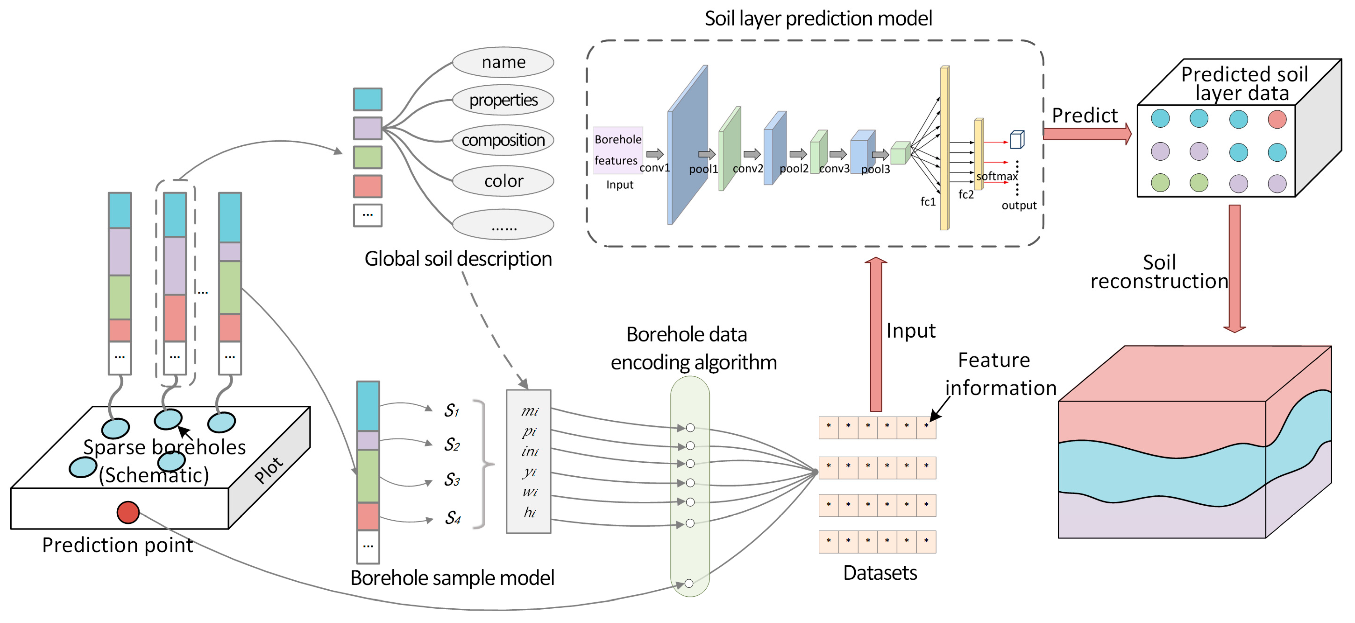
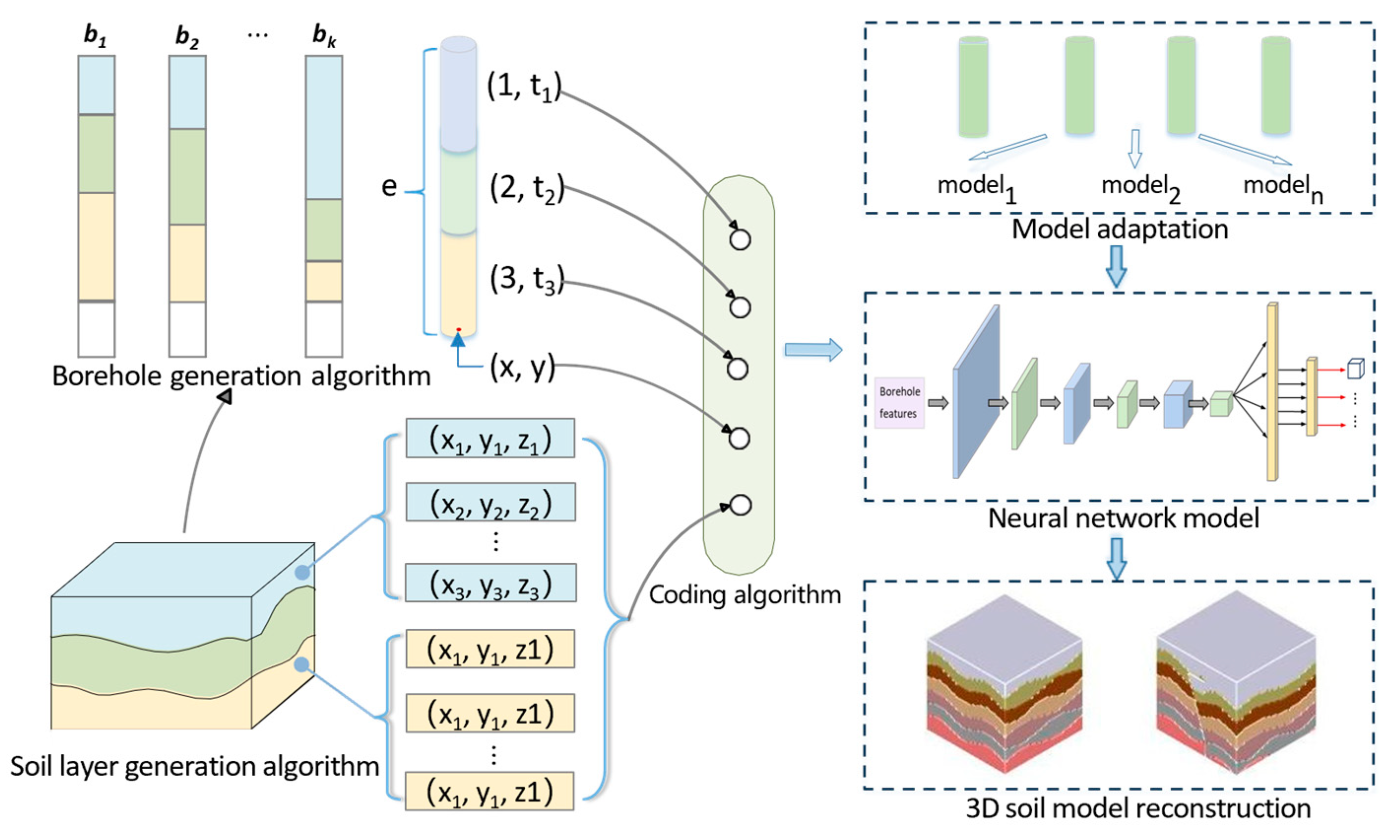
In response to the aforementioned problems, we designed a three-dimensional soil layer reconstruction method based on machine learning. The overall technical roadmap is shown in Figure 1. It is divided into five main technical links, including the following:

(1) Soil Layer Sample Data Enhancement Algorithm. In view of the scarcity of borehole data and soil samples, we designed soil layer data enhancement algorithms and borehole data enhancement algorithms to obtain sufficient training sample datasets;

(2) Borehole Data Preprocessing. An encoding algorithm is designed to encode borehole data with non-uniform dimensions into a feature map of a consistent form as an input to the network model;

(3) Deep Convolutional Neural Network Model Design and Training. We design and build a deep convolutional neural network model using the preprocessed borehole features as the input dataset. The model is trained and then saved for subsequent use;

(4) Model Adaptation Algorithm. A model adaptation algorithm is developed to fine-tune the model using a small amount of real borehole data provided by the user. The model is selected based on the number of soil layers to ensure it can be applied to modeling multiple soil layers;

(5) Visualization of Soil Layer Data. The voxel values are obtained from the soil layer labels output by the model. Voxels with the same label are clustered using a three-dimensional voxel aggregation algorithm, and the three-dimensional soil layer is generated through rendering.

2. Soil Layer Representation and Sparse Borehole Modeling

2.1. Meta-Information of Soil Layers

Real geological soil blocks contain multiple types of soil layers. Based on geological structural characteristics, they are primarily classified into continuous soil layers, hiatus soil layers, and fault soil layers. Based on soil properties, they can be further categorized into soft clay layers, expansive soil layers, collapsible loess layers, weathered rock layers, etc.

Table 1. Typical soil layer parameter information.

Scheme	Cohesion (kPa)	Internal Friction Angle (°)	Permeability Coefficient (m/s)	Common Engineering Issues
stiff clay	30–50	15–25	10−7–10−9	creep deformation
loose sand	0–5	25–30	10−4–10−5	quicksand
dense gravel	0	38–45	10−2–10−3	difficult dewatering
soft silt/mud	5–10	0–5	10−8–10−9	basal heave, large wall deflection
weathered rock	100–300	35–45	10−5–10−7	fracture water pressure

presents the types of soil layers that may be encountered during deep excavation, along with their corresponding characteristics and potential impacts on construction.

The information on soil layers mainly includes name, nature, composition, color, density, humidity, etc. The soil layer file is designed to store this information in this paper. Figure 2 shows the data structure of the soil layer file; the set of soil layers is denoted by $S$, $S=\left\{s_1,s_2,\dots ,s_n\right\}$, there are $n$ types of soil layers in $S$, and for $\forall si\in S$ there is a tuple, $si=\left\{m_i,p_i,{in}_i,y_i,w_i,h_i\right\}$, where $m_i$ represents the name of the $i$^th soil layer, $p_i$ represents the nature of the $i$^th soil layer, ${in}_i$ represents the composition of the $i$^th soil layer, $y_i$ represents the color of the $i$^th soil layer, $w_i$ represents the density of the $i$^th soil layer, and $h_i$ represents the humidity of the $i$^th soil layer.

2.2. Sparse Borehole Modeling

Borehole drilling refers to the method of drilling into the ground to investigate the distribution of subsurface soil layers. In engineering projects, borehole data are typically obtained through engineering drilling. When a borehole penetrates the ground, it passes through different soil layers, thereby revealing the thickness of each encountered layer. Borehole data include key parameters such as the elevation and coordinates of the borehole, the types of soil penetrated and their respective thicknesses, and other details like borehole radius, name, drilling time, color codes, etc. Borehole data are represented as a series of discrete points, with variations primarily observed in the vertical dimension. While vertical boreholes are the most common, inclined boreholes are also used in some cases. Utilizing these data allows for the direct acquisition of detailed soil distribution information and supports the creation of three-dimensional digital stratigraphic models. To accurately reconstruct soil layers, we designed a specific file format to systematically store and manage borehole data.

Figure 3 shows the structure of the borehole data. Each borehole file contains several boreholes, and the set of boreholes is represented by $B$, $B=\left\{b_1,b_2,\dots ,b_n\right\}$; there are $n$ boreholes in $B$; for all $b_i\in B$, there exists a tuple, $b_i=\left\{n,e,r,c,l\right\}$, where $n$ represents the name of the borehole, $e$ represents the elevation value of the borehole, $r$ represents the radius of the borehole, and $c$ represents the coordinates of the borehole. Here, $c$ is a tuple, $c=\left(x,y\right)$, where $x$ and $y$ are the coordinates of the X-axis and Y-axis directions of the borehole. $l$ represents the thickness of the soil layer and the soil layer through which the borehole passes, and $l$ is a nest tuple, $l=\left(\left(1,t_1\right),\dots \left(a,t_a\right)\right)$, where $\left(a,t_a\right)$ represents the label of the soil layer and the thickness of the soil layer through which the borehole passes.

Further, the borehole file also contains some other auxiliary information, such as file name, data type, file creation time, etc.

2.3. Voxel Data of Soil Layer

In three-dimensional space, the smallest unit of spatial volume is a voxel, which is represented by a single value. A voxel appears as a small cube in three-dimensional space. Voxel models have been widely applied in various fields, such as medical imaging [31], scientific visualization and simulation [32], and engineering applications [33]. We utilized a voxel model to build a three-dimensional terrain. The constructed soil model depends on the surface elevation and borehole data.

The basic steps are as follows: First, the block to be modeled is meshed. Then, the value of each voxel is calculated based on the label assigned by the model. This value represents its corresponding soil layer label. Next, the soil layer is generated using the voxel aggregation algorithm. Finally, the soil layer model is displayed in the visualization system with an appropriate orientation through the transformation matrix.

The soil voxel file is designed. The core part of the file is the voxel value. The set of voxels is represented by $V,V=$ $\left\{v_{s1},v_{s2},\dots ,v_{sn}\right\}$, where $v_{si}$ represents the voxel value set of the $i^{th}$ surface, $v_{si}=\left\{v_{l1},v_{l2},\dots ,v_{lm}\right\}$, where $v_{lj}$ represents the voxel set of the $j^{th}$ line in the $i^{th}$ surface, and $v_{\iota j}=$ $\left\{v_{ij1},v_{ij2},\dots ,v_{ijk}\right\}$, where $v_{ijp}$ represents the $p^{th}$ voxel value in the $j^{th}$ line of the $i^{th}$ surface. n, m, and k are the numbers of voxels in the X, Y, and Z directions of the soil layer after meshing, and their values depend on the length, width, and height of the stratum and the length, width, and height of the voxel. Figure 4 illustrates the process of soil layer visualization based on three-dimensional voxels.

Each soil layer voxel file has a collection $V$. The file assigns a specific color to each soil layer.

3. Data Enhancement Algorithm of Soil Layers

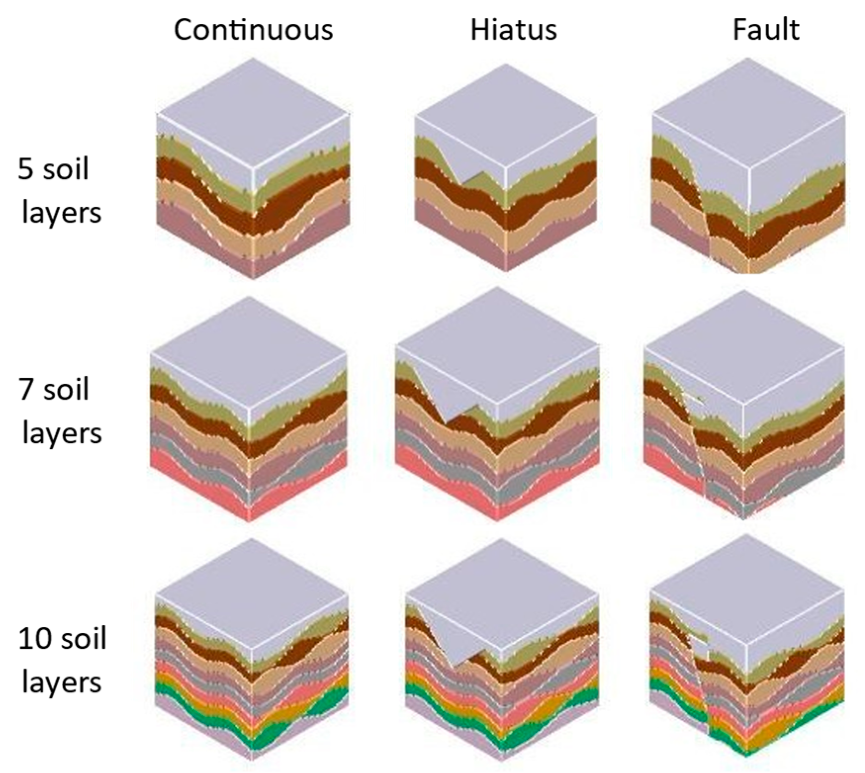
3.1. Common Patterns of Soil Layer Distribution

Over time, the occurrence of events such as crustal movement, weathering erosion, sedimentary discontinuities, and paleontological evolution significantly alters subsurface conditions. Based on an extensive review of geological data, we identified that soil layers can be primarily categorized into three types.

The first type is a continuous soil layer. This type of soil layer exhibits uninterrupted distribution, with no missing or disrupted layers, as illustrated in Figure 5a.

The second type is a hiatus soil layer. Due to the movement of the crust, the stratum lacks one or more layers of soil. It is usually in the shape of an inverted triangle. The remaining layers are still continuous. Figure 5b shows this situation.

The third type is a fault soil layer. Part of the crustal subsidence often leads to the formation of such a soil layer. The soil layer has a significant displacement fracture at a certain position, as depicted in Figure 5c.

In a continuous soil layer, the interface between the two types of soil also rarely appears in the form of a plane. Instead, they typically are curved surfaces. In addition to continuous soil layers, geological processes have also formed soil layers with hiatuses and faults. Based on this information, we simulated the formation process of real soil layers on Earth. Additionally, we designed a soil layer generation algorithm capable of generating data for the aforementioned three types of soil layers.

3.2. Soil Layer Generation Algorithm

The purpose of the algorithm is to simulate the real soil layer generation process, generate simulated soil layer data, and expand the training dataset for soil layers. In practical engineering, soil layer modeling typically relies on borehole data. However, due to the scarcity of borehole data, the resulting soil layer datasets are often small. Therefore, we designed a soil layer generation algorithm to acquire a sufficient amount of data.

The algorithm dynamically generates three types of soil layers based on varying input parameters. It allows customization of the thickness and proportion of each soil layer, thereby enhancing soil layer diversity. When generating hiatus soil layers, the coordinates of the hiatus plot are entered, and when generating fault soil layers, the coordinates of the fault and the thickness of the fault are entered.

In this algorithm, the following definitions are introduced:

Definition 1 (Stratum elevation). 

The elevation is the height of the stratum in three-dimensional space, denoted by $E$.

Definition 2 (Rectangular bottom vertex coordinate set of the stratum). 

The bottom vertex coordinate set is the polygon vertex coordinates at the soil layer’s bottom, represented by the set $D$, where $D=\left\{d_1,d_2,\dots ,d_n\right\}$. For each $d_i\in D$, $d_i$ is defined as $\left\{x_i,y_i\right\}$, where $x_i$ and $y_i$ are the coordinates of the $i$^th vertex in the X and Y directions, respectively.

Definition 3 (Three-dimensional grid). 

A three-dimensional grid divides three-dimensional entities in space. In our algorithm, the three-dimensional grid is conceptualized as a small cuboid and represented by the tuple $G$, where $G=\left\{g_1,g_2,g_3\right\}$. Here, $g_1$, $g_2$, and $g_3$ represent the length, width, and height of the cuboids in the grid, respectively.

Definition 4 (Soil layer proportion). 

The soil layer proportion refers to the ratio of the average thickness of each soil stratum to the total thickness across all layers. This parameter’s design can enhance the diversity of generated soil layer configurations. The proportion is denoted by the set $L=\left\{L_1,L_2,\dots ,L_{num}\right\}$, where $L_i$ represents the proportion of the $i^{th}$ soil layer, ensuring that ${\sum }_{i=1}^{num}{L}_i=1$.

Definition 5 (Hiatus coordinate set). 

The hiatus coordinate set represents the triangular vertex coordinates of the missing portion of the soil layer projected onto the XZ plane. It is defined as an ordered set, $S_h=\left\{S_{h1},S_{h2},\dots ,S_{hn}\right\}$, where each $S_{hi}$ denotes the coordinates of the $i$^th vertex. Here, $S_{hi}$ is a binary tuple, $S_{hi}=\left(s_{hx},s_{hz}\right)$. As shown in Figure 5b, the hiatus soil layer typically forms an inverted triangular shape, with the vertices labeled as points A, B, and C defining the boundaries of the missing region.

Definition 6 (Fault soil layer coordinate set). 

The fault soil layer coordinate set represents the endpoint coordinates of the line segment projected by the fault portion of the soil layer onto the XZ plane. It is defined as an ordered tuple, $S_s=\left\{S_{s1},S_{s2}\right\}$, where each $S_{si}$ denotes the coordinates of the $i$^th endpoint. Here, $S_{hi}$ is a binary tuple, $S_{si}=\left(s_{sx},s_{sz}\right)$. As shown in Figure 5c, the coordinate set of points A and B is $S_s$, which defines the boundaries of the fault line segment.

Definition 7 (Fault soil layer subsidence height). 

This term describes the height of the whole soil subsidence on one side of the fault line segment, symbolized as $d_s$.

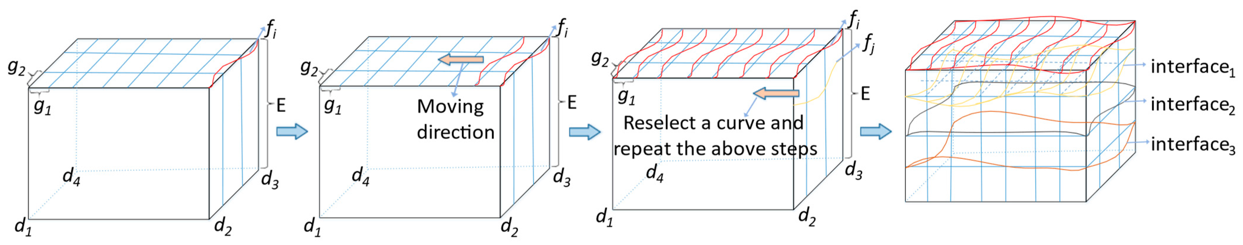
Definition 8 (Smooth curve function set). 

A set of functions designed to generate smooth surfaces, represented by the set $F=\left\{f_1,f_2,\dots ,f_n\right\},$ where $f_i$ is a B-spline curve function. Each curve has $g_f$ control points determined by Formula (1). The coordinate pi of each control point is selected randomly up or down by the grid point where the curve is located. These curves serve to replace straight lines within the grid.

$$g_f={\displaystyle \frac{\left|y_2-y_1\right|}{2g_2}},$$

(1)

where $y_1$ and $y_2$ are the $y$ coordinates of the polygon vertex in the Y-axis direction, and $g_2$ is the width of the three-dimensional grid.

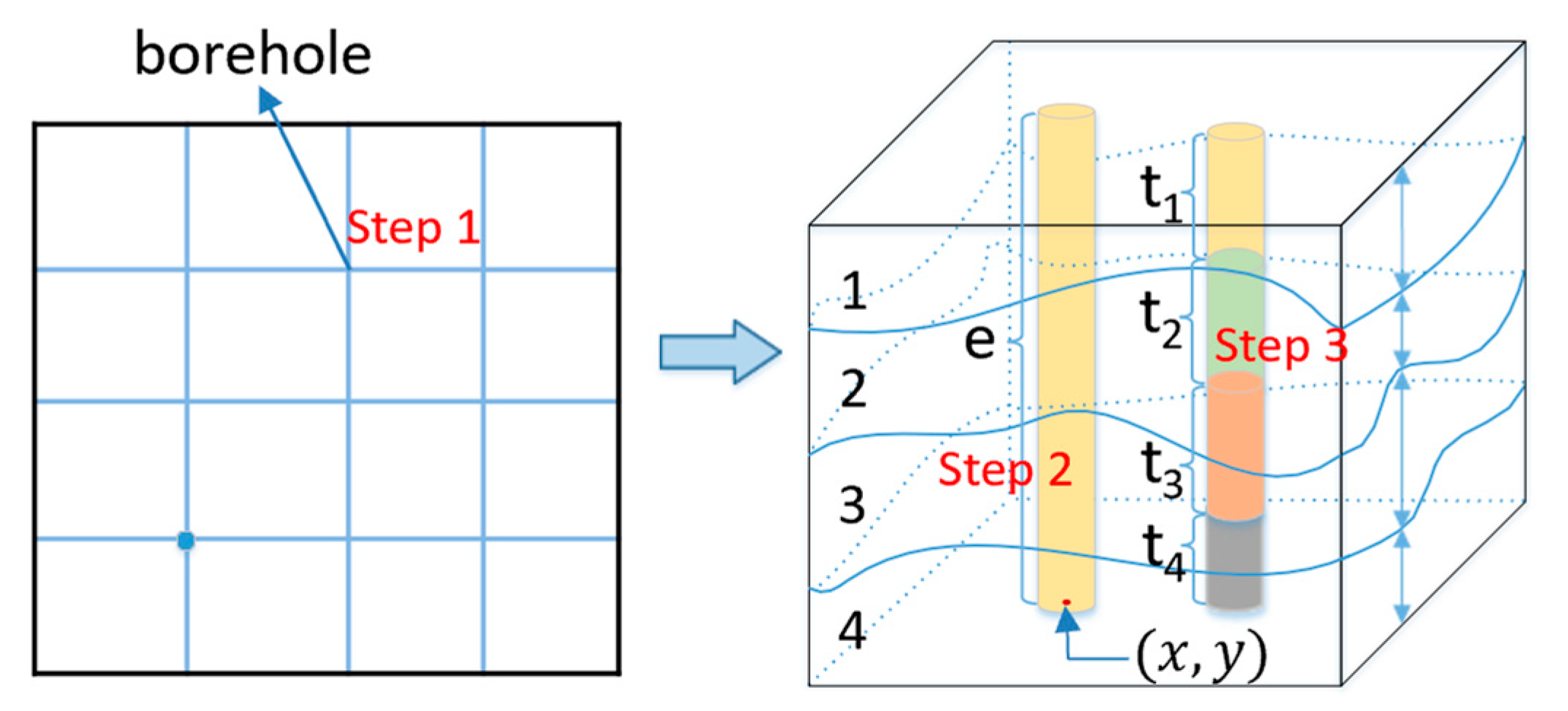
As shown in Figure 6, the continuous soil layer generation algorithm is divided into four steps, as follows:

Step 1. Generate a seed curve: For all $f_i\in F$, use the top point set of the soil layer grid as the input of $f_i$, and solve the function $z_i=f_i\left(y_i\right)$ to acquire the new height coordinate of the grid point. Then, the Z coordinate point of the grid point is replaced by $z_i$.

Step 2. Move the seed curve: Using the $f_i$ selected in the first step, select the grid points on $z_i$-$g_i$ in the same layer. Solve the function $z_i=f_i\left(y_i\right)$ and generate the second curve, thereby obtaining the updated coordinates $z_i$.

Step 3. Generate the first layer of the surface: Use the grid points on $z_i$-$g_1$ as the input of the function $f_i$ in turn, and repeat step 2 until the first layer of the surface is generated.

Step 4. Generate all boundary surfaces: Re-select the function $f_i$ from set $F$ and repeat the first three steps until all boundary surfaces are generated.

After the soil layer interface is generated, the mesh points enclosed by this interface are categorized as belonging to the same type of soil layer, and this portion of voxel data is saved. For continuous soil layers, $S_h$ is input to retrieve hiatus soil layer data. Then $S_s$ and $ds$ are input to obtain fault soil layer data. The process for creating a hiatus soil layer involves removing a portion of the voxel data from the continuous soil layer to form a ‘sink’. Conversely, the fault soil layer process involves subtracting a constant value from the height coordinates of a segment of the voxel data in the continuous soil layer to create a ‘section’, while the rest of the soil layers remain in their continuous state.

The generated soil layer data are represented by the set $T=\{t_1,t_2,\cdots ,t_n\}$, where $T$ contains $n$ soil layers. For all $t_i\in T$, there is a set $t_i=\{w_1,w_2,\dots ,w_n\}$, where $w_i$ is the three-dimensional coordinates of grid point $i$. Each $w_i$ is an array defined as $w_i=\left(w_{px},w_{py},w_{pz}\right)$.

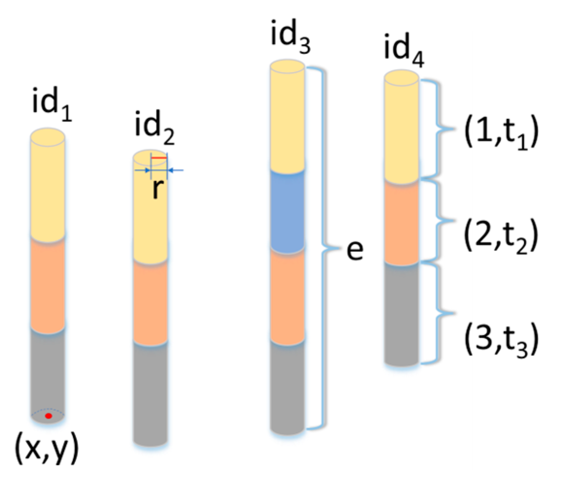
3.3. Generation Algorithm of Virtual Boreholes

Based on the soil layer data, we designed a borehole generation algorithm. The borehole locations are randomly selected from the uppermost grid points of the soil layer. First, the positions of the boreholes are determined based on these grid points. Subsequently, a set of boreholes is randomly generated according to the soil layer characteristics, and the thickness of each layer at each borehole location is calculated using the interface coordinates between the layers. The schematic diagram of the algorithm is illustrated in Figure 7.

The borehole generation algorithm consists of three steps:

Step 1. Select the grid point coordinates. The positions of the boreholes are all taken on the grid points.

Step 2. Acquire the borehole elevation and plane coordinates. The borehole elevation is the height coordinate of the grid point. We use the plane coordinate of the selected grid point as the borehole coordinate.

Step 3. Parse the soil layer that the borehole passes through from the soil layer data and extract the label of the soil layer. Then, calculate the thickness of each identified soil layer using the formula provided in Formula (2).

$$thicknes{s}_i=z_i-z_{i+1},$$

(2)

In the above formula, ${thickness}_i$ is the thickness of the $i^{th}$ soil layer at the borehole location; $z_i$ is the height coordinate value of the grid point through which the borehole passes at the $i^{th}$ interface; and $z_{i+1}$ is the height coordinate value of the grid point through which the borehole passes at the ${\left(i+1\right)}^{th}$ interface.

The generated borehole data are represented by the set $Z$, where $Z=\{z_1,z_2,\dots ,z_n\}$. This set $Z$ contains $n$ boreholes. For each $z_i\in Z$, there exists a set $z_i=\{e_{pi},l_{pi},t_{pi},c_{pi}\}$, where e_pi is the elevation value of the $i^{th}$ borehole, l_pi is the soil layer through which the $i^{th}$ borehole passes, t_pi is the thickness of each soil layer through which the $i^{th}$ borehole passes, and c_pi is the plane coordinate of the $i^{th}$ borehole.

4. Machine Learning Models for Soil Layer Reconstruction

4.1. Sparse Borehole Encoding

A large amount of soil layer and borehole data can be obtained through the soil layer generation algorithm and the borehole generation algorithm. However, this information cannot be directly used as the characteristics of the soil layers to train the network. To reconstruct a 3D soil layer model, it is essential to determine the attributes of each voxel within the soil layer being modeled. This involves dividing the soil layer into a three-dimensional grid and using the grid points as sample locations. Given the deterministic nature of the soil layer generation algorithm, each sample point belongs to a unique soil layer type, thereby defining its label. To characterize these samples, we devised an encoding method that links borehole data with the sample points, facilitating the acquisition of their properties.

The algorithm has the following definition:

Definition 9 (Sample points of soil layer). 

These are three-dimensional grid points. The method of selecting sample points is to randomly select the entire soil layer grid. The coordinates of sample points are represented by P, P = (X, Y, Z).

Definition 10 (Borehole dimension). 

The borehole dimension is the amount of data contained in a borehole. It is represented by Z_d. It can be known from the borehole generation algorithm that the borehole data consist of four sets of data.

If there are a total of three data amounts for the borehole coordinate and elevation, then the dimension of the borehole is calculated according to Formula (3):

$$z_d=n_s+3,$$

(3)

where $n_s$ represents the number of soil layers penetrated by a borehole.

The schematic diagram of the algorithm is presented in Figure 8. The algorithm procedure is divided into three main steps, as outlined below:

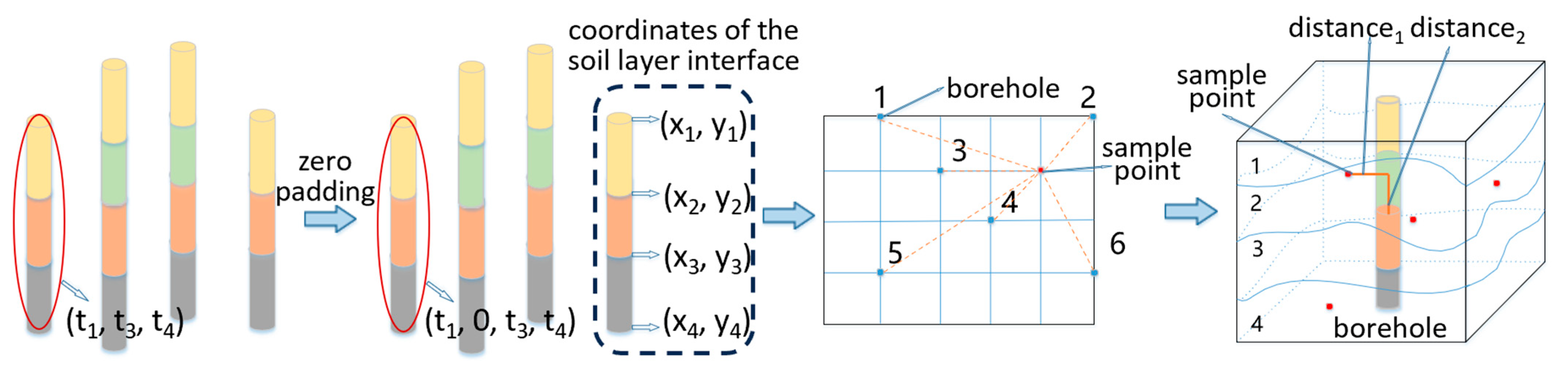
Step 1. Uniform Borehole Dimension. Due to the presence of hiatuses and faults in soil layers, boreholes passing through these layers may lack thickness information for certain soil layers. Since the number of missing layers can vary, the dimensions of borehole data may become inconsistent. This inconsistency results in a mismatch between the dimensions of sample features and the input requirements of neural network models. To resolve this issue, we apply zero-padding to the missing data layers, assigning a thickness value of zero to the positions where borehole data are absent.

Assuming the number of soil layers that need zero-padding is $Z_b$, then $Z_b$ can be derived from the following formula:

$$z_b=\left\{\begin{array}{ll}{s}_{num}-n_s,\hfill & n_s<s_{num}\hfill \\ 0,\hfill & n_s\ge s_{num}\hfill \end{array}\right.,$$

(4)

where $n_s$ is the number of soil layers passed by a borehole; $s_{sum}$ is the number of generated soil layers input in the algorithm.

Step 2. Acquiring the Coordinates of the Soil Layer Interface at the Borehole Position. After determining the thickness of the soil layer, the spatial distribution information of the soil layer is required. This spatial information is described by the coordinates of the soil layer interface. As derived from the borehole generation algorithm, the thickness of the soil layer is calculated based on the height coordinates of the boundary surface at the borehole position. The height coordinates of the soil interface at the borehole position can be obtained using Formula (5).

$$z_{sn}={\displaystyle \sum _{i=1}^{n-1}{h}_i},$$

(5)

where $h_i$ is the thickness of the $n^{th}$ soil layer; $Z_{sn}$ is the height coordinate of the interface between the $n^{th}$ soil layer and the ${(n+1)}^{th}$ soil layer at a borehole location.

Step 3. The distance from the soil layer boundary point to the sample point is calculated: We select the k boreholes closest to the sampling point and then obtain the coordinates of the soil interface at the borehole location. Subsequently, both the horizontal (distance1) and vertical distances (distance2) from these interface points to the sample point are computed.

For a sample point $P$, the distance from all boreholes to it is first calculated. This set of distances is represented by an ordered set, $J=\{j_1,j_2,\dots ,j_n\}$. In this set, each $j_i$ represents the horizontal distance from the $i^{th}$ borehole to the sample point $P$. The elements of set $J$ are arranged in ascending order and the first $k$ elements are selected. In Figure 8, boreholes 2, 3, 4, and 6 are the four closest boreholes to the sample point. Next, the coordinates of the points where these boreholes intersect with the soil layers are calculated. According to the Euclidean distance formula, distance₁ and distance₂ can then be calculated.

After these three steps, all the feature data of a sample can be generated, including the information on several boreholes, and the information on each borehole contains six sets of data, namely the elevation of the borehole, the coordinates of the borehole plane, the thickness of the soil layer, the coordinates of the soil interface at the borehole location, the horizontal distance from the coincidence point to the sample point, and the vertical distance from the coincidence point to the sample point, as shown in Figure 9. The dimension of a sample is determined by the number of soil layers ($s_{sum}$) and the number of selected boreholes (k). The calculation formula is as follows:

$$D_s=(4S_{num}+6)k,$$

(6)

4.2. Prediction Model

Deep convolution plays an important role in the feature extraction of high-dimensional data. This paper uses a deep convolutional neural network as the basic reconstruction model structure. The specific structure of the model contains three convolutional layers and two fully connected layers. The model can choose to set the hyperparameters used to determine the network architecture, in which the activation function applies Rectified Linear Unit (ReLU), and the pooling method uses maximum pooling.

In real-world scenarios, soil layer distributions are highly variable, and the number of soil layers is not constant. However, the trained model can only be modeled for soil layers with a constant number of layers. If a prediction model is designed for each number of layers, this will make the number of models very large and consume a lot of resources.

Therefore, we designed a model adaptation algorithm to preprocess the borehole data. The model can be applied to geology modeling with different soil layers. Figure 10 shows the operation steps of this algorithm.

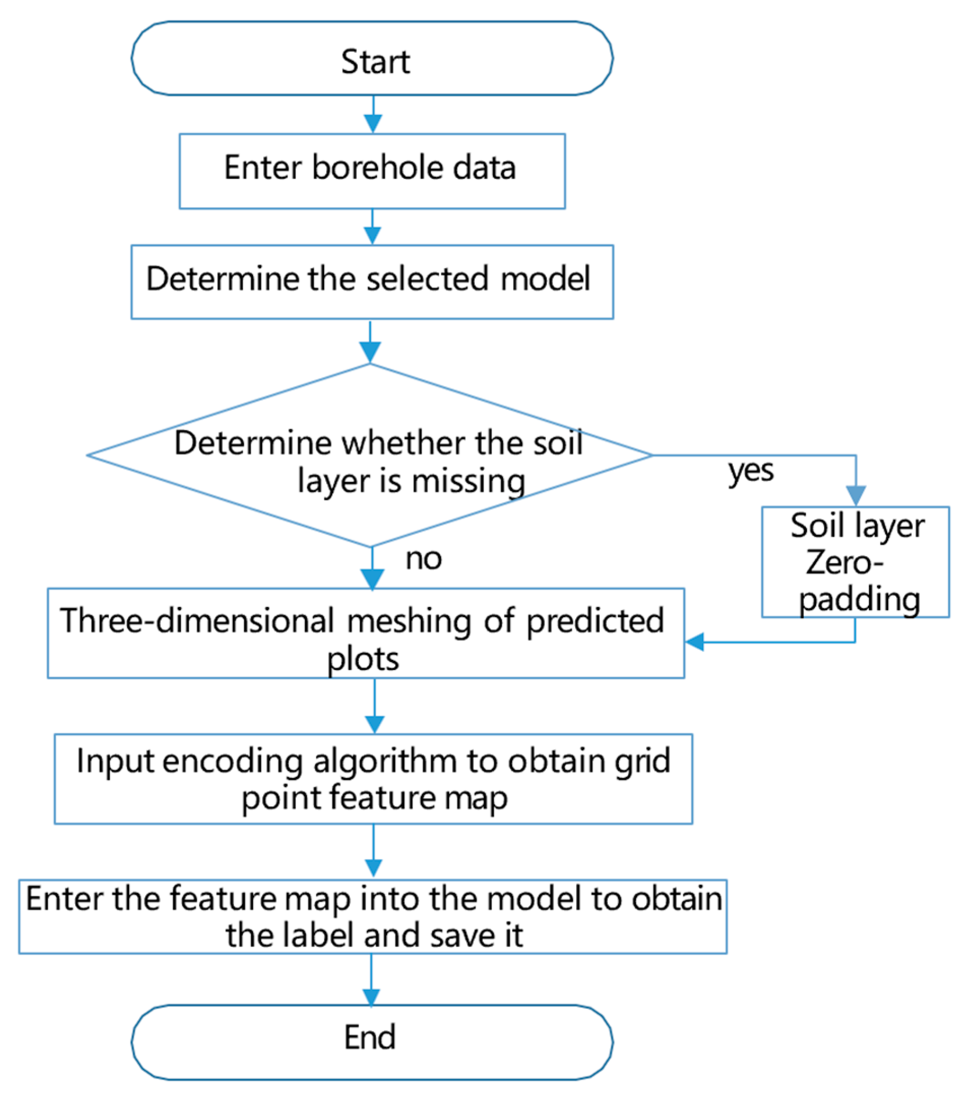
The model adaptation algorithm is divided into three steps:

Step 1. Selection of the trained soil layer reconstruction model. According to the borehole data provided by the user, the number of soil layers $S_{num}$ to be modeled is determined, and then the model is selected according to the number of soil layers. The selection method is as follows:

$$M=\left\{\begin{array}{cc}{M}_1,\hfill & 0<s_{num}\le m\hfill \\ M_2,\hfill & m<s_{num}\le 2m\hfill \\ \dots \hfill & \hfill \\ M_n,\hfill & \left[{\displaystyle \frac{n}{m}}\right]m<s_{num}\le n\hfill \end{array}\right.,$$

(7)

where n is the maximum number of soil layers, and m is the step size.

Step 2. Zero-padding treatment of the soil layer. To ensure consistency with the model’s input requirements, zero-padding is applied to all borehole data corresponding to the missing layers. This process standardizes the number of soil layers across all borehole data to match the model’s expected input dimensions.

Step 3. Prediction of voxel values. The preprocessed borehole data are input into the encoding algorithm, which divides the formation to be modeled into grid points. The feature map for each grid point is generated based on the encoding algorithm. Subsequently, the feature maps are fed into the model for prediction, yielding the corresponding label values.

In a typical low-quality environment for foundation pit construction, the number of soil layers is usually no more than 10. Therefore, this paper sets n to 10 and m to 5, then designs and trains two models with the numbers of soil layers corresponding to 5 and 10, named SCNN-5 and SCNN-10, respectively. If the soil layer type in borehole sampling is less than or equal to five, SCNN-5 is used for soil layer prediction. When the number of soil layers is greater than five, SCNN-10 is used. 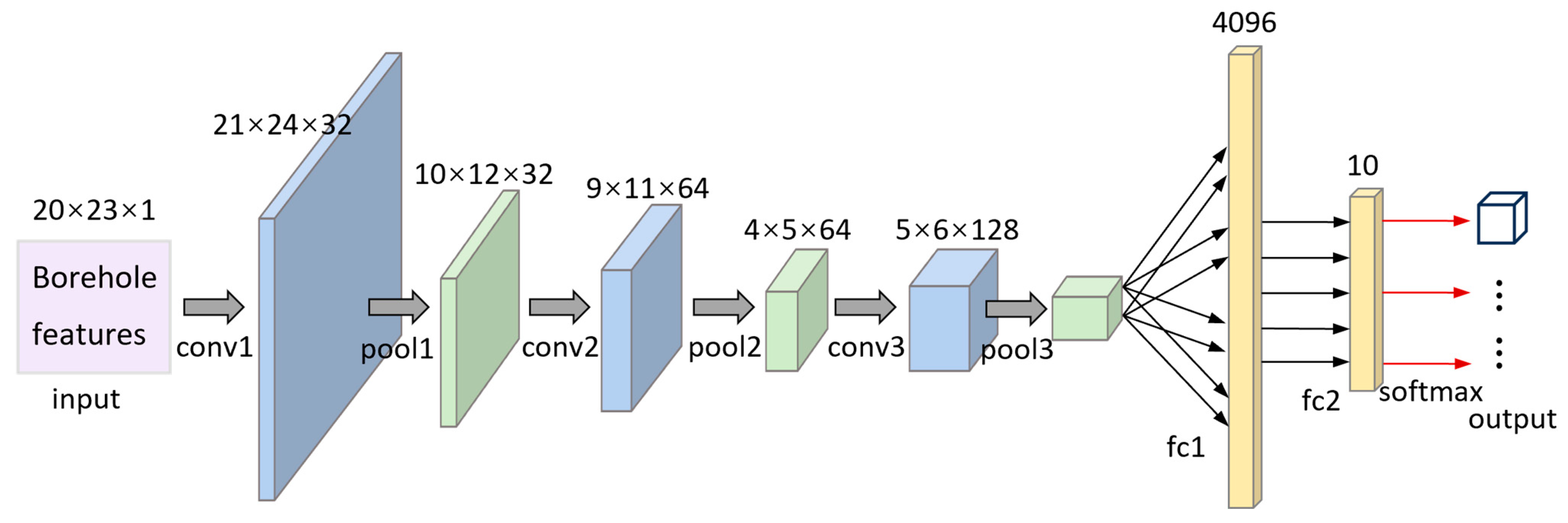Figure 11 shows the structure of SCNN-10.

Our CNN includes three convolutional and two fully connected layers. The distribution of label information is achieved by applying the output of the second fully connected layer to the input of the 10-way softmax layer. Borehole features with dimensions of 20 × 23 × 1 are applied to the input layer. All convolutional layers consist of four stages in order, namely convolution, ReLU, normalization, and pooling, followed by a 4096-node fully connected layer containing two stages: an inner product and ReLU. Additionally, convolutional layers 1–3 consist, respectively, of 32 feature maps with a filter size of 2 × 2, stride of 1, and padding of 1; 64 feature maps with a filter size of 2 × 2, stride of 1, and padding of 0; and 128 feature maps with a filter size of 2 × 2, stride of 1, and padding of 1. The first fully connected layer consists of 4096 nodes, while the second one consists of 10 nodes, followed by the softmax classification layer.

Through small-scale preliminary experiments, the model structure adopted by the algorithm was found to be sufficient to capture the key features in the soil layer data, while ensuring computational efficiency and avoiding overfitting. The model with two convolutional layers exhibited lower accuracy and did not meet practical requirements. In contrast, compared to the three-layer model, the framework models with four and five layers achieved an accuracy improvement of approximately 3%, but their computation times increased to about 1.4 and 1.8 times that of the original model, respectively, with a significantly increased risk of overfitting.

We also conducted a hyperparameter tuning process to achieve better model performance. The final parameter settings are as follows. Activation function: ReLU; all layers use the ReLU activation function. Optimizer: Adam; we employ the Adam optimizer with a learning rate of 0.001. Training iterations: 20,000; the model is trained for 20,000 iterations. Batch size: 128; a batch size of 128 is used during training. Dropout rate: 0.5; a dropout rate of 0.5 is applied after each pooling layer to help prevent overfitting. Weight decay: 1 × 10⁻⁴; a weight decay of 1 × 10⁻⁴ is used for regularization.

4.3. Datasets and Model Training

Corresponding to the two models, we designed two datasets to train them, respectively. The borehole data processed by the coding algorithm were used as the feature data for the samples. Given that the data from each part do not fall within the same range, it is necessary to standardize the feature data to ensure all data are in the same range. For this purpose, the Gaussian function was utilized for normalization.

The standardized feature data were compiled into separate datasets for different terrains. Each dataset has distinct sample sizes and dimensions. To ensure that samples could be taken from all soil layers, several points were randomly selected from within each layer. The sample sizes of the datasets amounted to 100,000 and 120,000, as shown in

Table 2. Dataset sample size and sample dimensions.

Number of Soil Layers	Sample Size	Sample Dimension
5	100,000	260
10	120,000	460

. In both datasets, the training set accounted for 70%, while the test set comprised the remaining 30%.

In the process of training our models, we utilized data samples generated by both the soil layer generation algorithm and the borehole generation algorithm. This data augmentation technique enabled us to obtain a substantial amount of sample data, which were then processed through the encoding algorithm before being fed into the network models. When applying these models in real-world engineering scenarios, actual borehole data are inputted into the corresponding model via a model adaptation algorithm. Figure 12 provides a detailed illustration of this workflow.

During the training process, data flow through each learning layer, and the loss value is ultimately calculated using the cross-entropy function. A smaller loss value indicates higher convergence of the neural network model and increased accuracy. The network model optimizer employs the Adam optimizer. To prevent overfitting, a dropout function is applied after each pooling layer to randomly deactivate neurons. The cross-entropy operation is performed on the real values and predicted values to compute the error, which leads to continuous updates of the weight and bias parameters. The training involves 20,000 iterations, and

Table 3. Test accuracy of the model on the dataset.

Number of Soil Layers	Sample Size	Test Accuracy
5	100,000	92%
10	120,000	95%

shows the accuracy of the model on the test set.

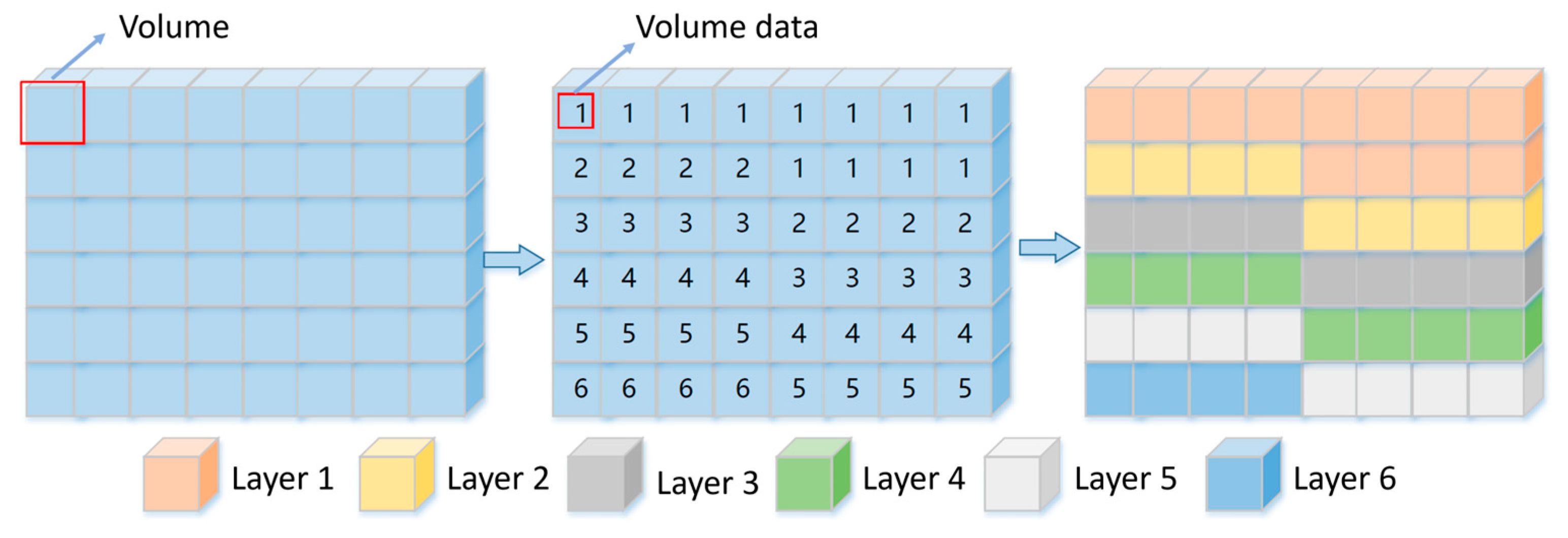
The label returned by the network model represents the value of a voxel, with each voxel corresponding to a small block of soil. The three-dimensional voxel aggregation algorithm aggregates voxels with identical soil characteristics into a unified structure. This 3D voxel aggregation technique allows for storing connected soil layers in a list. The algorithm employs principles similar to those of the maze algorithm, a classic approach used for path planning. Maze algorithms can be categorized into depth-first search, breadth-first search, genetic algorithms, and ant colony algorithms. Currently, many scholars opt to optimize the maze algorithm for path-planning applications [34]. In this paper, we utilize a depth-first search approach for path planning. After aggregating all connected voxels, we reconstruct the surface using an isosurface extraction method and then render it as a soil model. The resulting soil layer generated by our model is visualized in the system shown in Figure 13.

5. Experimental Evaluation

In the algorithms for soil layer generation and coding, numerous dynamic parameters are defined. The choice of these parameters significantly influences the prediction model’s performance. Consequently, it is essential to fine-tune these parameters to their optimal ranges to achieve the best possible model performance. Within our coding algorithm, we devised an experiment to investigate how the number of boreholes surrounding a sample point impacts the outcome. Furthermore, two experiments on the model were conducted: one comparing the model presented in this study with other models and another validating the model adaptation algorithm.

5.1. Experimental Results

(1) Experimental Study on the Impact of Borehole Numbers

During the development of the coding algorithm, we selected multiple boreholes surrounding a sample point for data encoding. Recognizing that the number of these boreholes significantly influences model quality, we conducted a series of experiments aimed at identifying the impact of different borehole numbers on model quality. In our study, we utilized SCNN-5 and SCNN-10 network models. Our methodology involved selecting the borehole closest to the sample point, encoding its data using the specified algorithm, and subsequently evaluating the accuracy of our test set through neural network analysis. The outcomes of our experiments are summarized in

Table 4. Results of different numbers of boreholes.

Model	7	8	9	10	11	12	13
SCNN-5	87%	87%	89%	92%	92%	88%	84%
SCNN-10	86%	93%	94%	95%	92%	90%	89%

, showing the impact of varying borehole numbers on model performance.

(2) Model Performance Comparison

To test the performance of the model, several classic classification algorithms were selected for comparison, including the LSTM neural network, random forest, decision tree, and SVM classifier. Each algorithm was tested using both 5-category and 10-category datasets. The results are shown in

Table 5. Results of different models.

Categories	SCNN-5	SCNN-10	Decision Tree	Random Forest	SVM	LSTM
5 categories	92%	/	82%	85%	87%	90%
10 categories	/	95%	79%	82%	86%	91%

.

(3) Model Adaptation Algorithm Performance Verification

In this part, to enhance the adaptability of the model, a model adaptation algorithm was designed. This approach utilized two models to address classification problems spanning 1 to 10 different categories. Missing soil layer data were handled by performing zero-padding.

Within this section, classification models for scenarios 3, 4, 7, and 8 were developed. Regarding the missing layer borehole data, the performance of the classification models for scenarios 3 and 4 was compared against SCNN-5. Similarly, the performance of the classification models for scenarios 7 and 8 was compared with SCNN-10. The experimental results are summarized in

Table 6. Model adaptation algorithm performance verification.

Model	3	4	7	8
Corresponding model	86%	89%	78%	90%
SCNN-5	84%	89%	/	/

.

(4) Real-world Application and Simulation Results

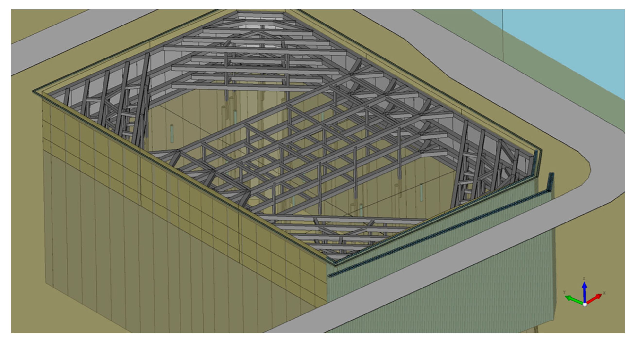
To further validate the practical applicability of our proposed method, we applied the algorithm to a real-world foundation pit project. The project is located in an urban area of a city in China. The geological conditions within the foundation pit site are complex, with soil layers composed of artificial fill, silty sand, silt, and clay. The excavation has an overall hexagonal shape, measuring approximately 75 m in the east–west direction and 119 m in the north–south direction, with a perimeter of 378 m and a depth of about 19.45 m.

Additionally, a main building structure with a basement is situated approximately 35 m east of the excavation site. To the south, a subway tunnel runs nearby, with a minimum distance of about 15 m from the excavation edge. The tunnel has an inner diameter of 8.5 m and is buried approximately 5.3 m below the excavation bottom. These factors significantly increase the construction difficulty and risks.

To enhance risk assessment and optimize the support system design, soil layer reconstruction is essential for such engineering projects. The excavation layout is illustrated in Figure 14.

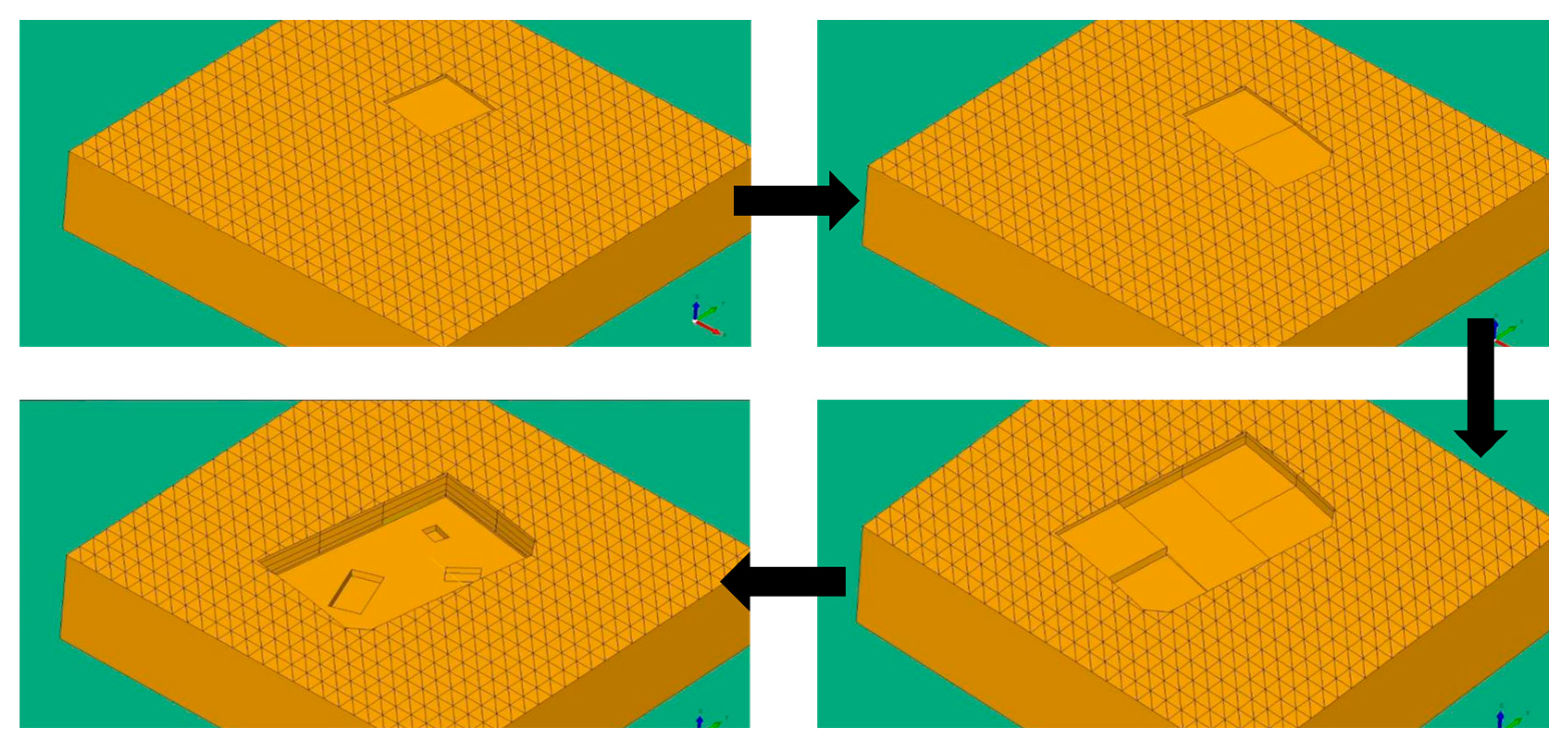
Before construction, the soil layer model reconstructed using this algorithm can be used for simulating the support structure construction and the excavation process. By calculating the relevant mechanical responses, a predictive analysis of the construction process can be conducted, which helps determine the foundation pit support structure.

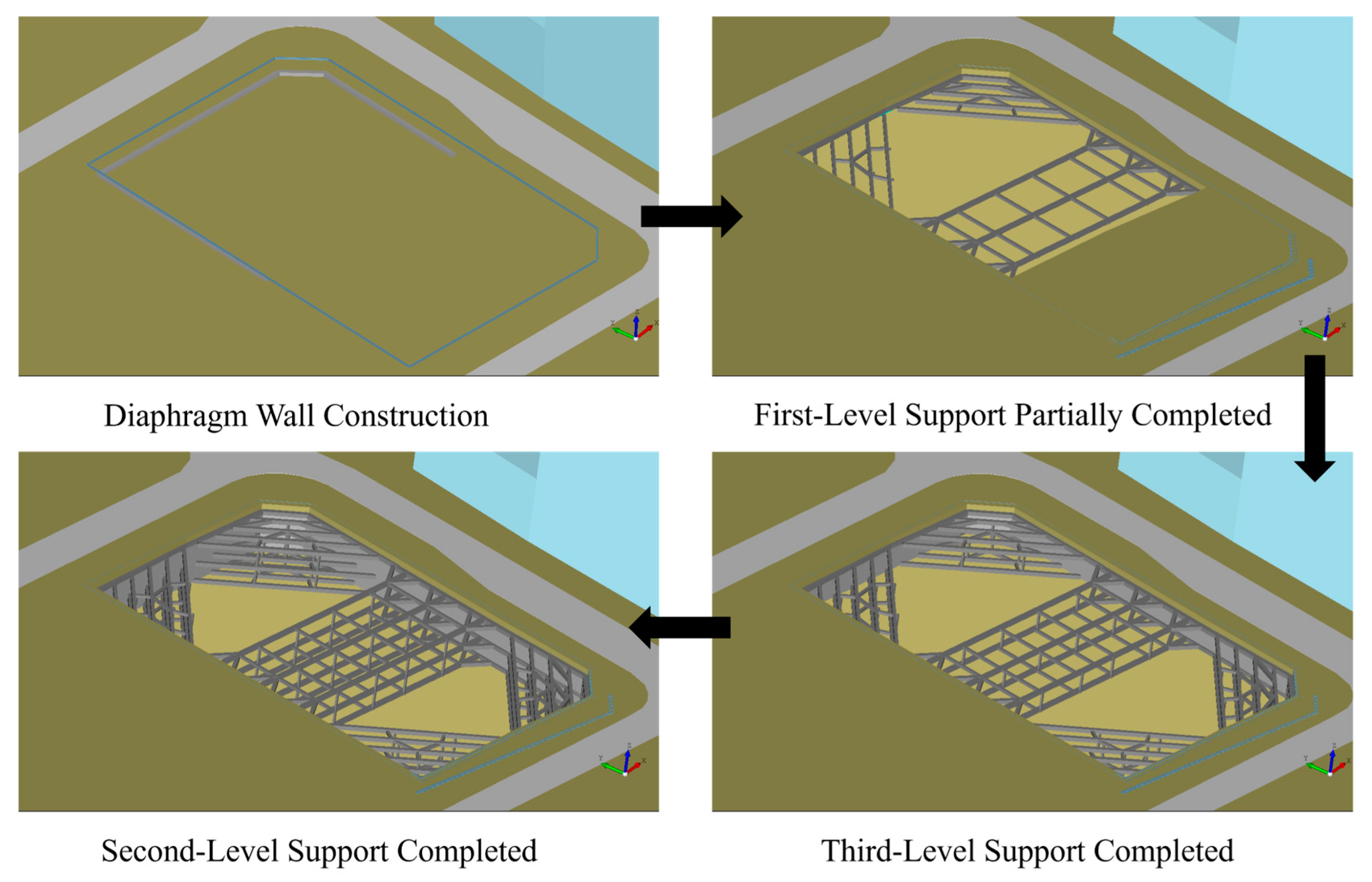
Figure 15 illustrates the three-dimensional soil layer reconstruction result obtained using our algorithm. The reconstructed model accurately captures the spatial distribution of soil layers, including continuous, hiatus, and fault layers, involving various types of soil, demonstrating the robustness of our approach in handling complex geological conditions. Figure 16 presents the simulated construction effects, which include the support structure of the excavation pit. The simulation results provide valuable insights for risk assessment and construction planning, highlighting the practical utility of our method in real-world engineering scenarios.

After excavation, based on the reconstructed soil layer model, the earthwork excavation process can also be recorded. The three-dimensional soil layer model, combined with monitoring data, enables real-time visualization and early warning of multi-source monitoring data. The construction team can use dynamic information to promptly reinforce the support structure or adjust the construction plan. Figure 17 and Figure 18 illustrate the construction of the support structures and the excavation process, along with progress tracking during the deep foundation pit excavation.

5.2. Analysis and Discussion

(1) Experimental Study on the Impact of Borehole Numbers

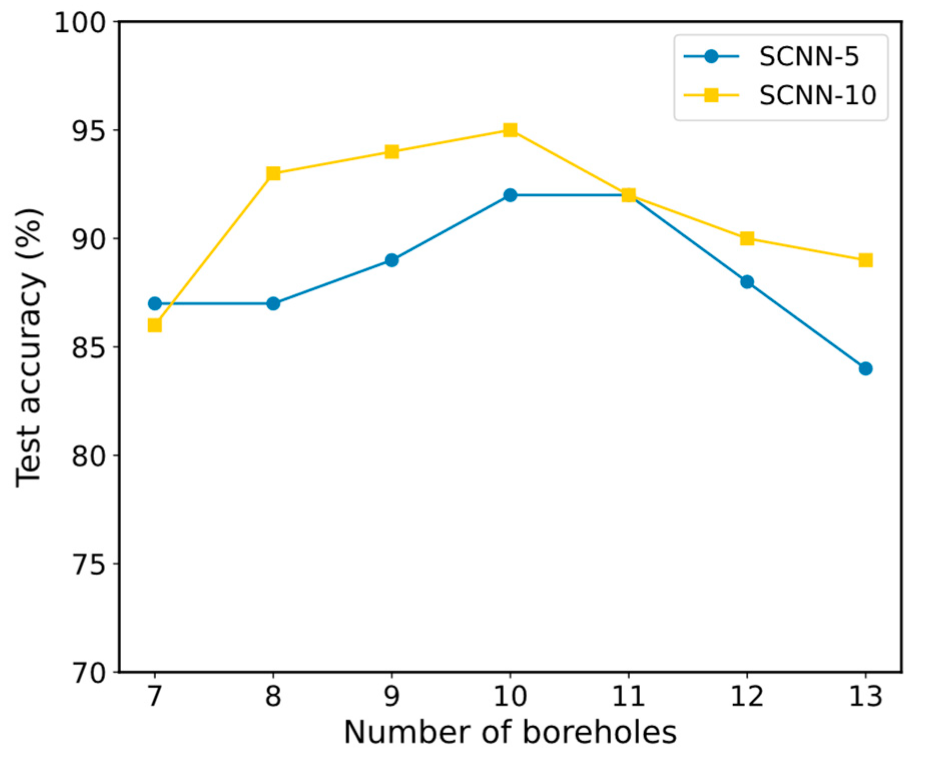
The experimental results for the number of boreholes selected are shown in Table 4, and the corresponding line graph is shown in Figure 19.

Figure 19 illustrates the relationship between the number of boreholes chosen and the quality of the model. Both models achieve their best performance with 10 boreholes, reaching accuracy rates of 92% and 95% on the test set. The line graph also shows that when the number of boreholes ranges from 7 to 13, the models demonstrate notable effectiveness, with accuracy exceeding 80%. According to the coding algorithm used, changes in the number of boreholes alter both sample dimensions and characteristics, which impacts the network model’s ability to extract features and, consequently, its performance on the test set. Based on the experimental results for the coding algorithm proposed in this paper, the optimal value of $k$ is 10.

(2) Model Performance Comparison

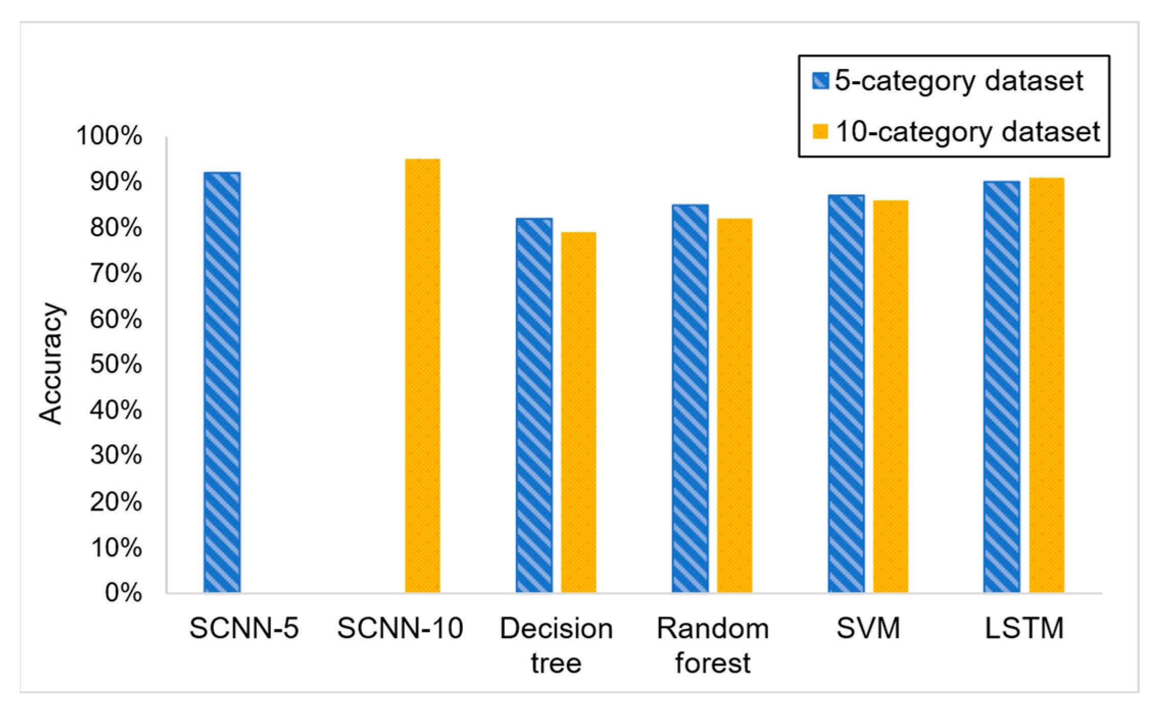
The performance comparison experiment results of different machine learning methods on the test set are shown in Table 5, and the histogram obtained from this table is shown in Figure 20.

Based on the experimental results, we can conclude that the network model proposed in this paper performs optimally across various datasets. Specifically, within the five soil layer datasets, SCNN-5 achieves the highest test accuracy, with other categories also demonstrating accuracies surpassing 80%. Among the models evaluated, the LSTM neural network follows SCNN-5 in performance, reaching an accuracy of 90%. For datasets containing ten soil layers, SCNN-10 exhibits superior performance; however, both the decision tree and random forest models show a decline in effectiveness. This discrepancy is likely attributed to the increase in sample feature complexity and dataset size. In contrast, SCNN-10 thrives under these conditions, suggesting that deep convolution operations are particularly effective for feature extraction in complex datasets. These findings highlight the robustness of the proposed SCNN model in handling varied and complex data environments.

(3) Model Adaptation Algorithm Performance Verification

The experimental results of model adaptation algorithm performance verification are shown in Table 6. The histogram obtained from this table is shown in Figure 21.

As can be seen from the figure, after applying the model adaptation algorithm, the performance of the models SCNN5 and SCNN-10 is similar to the performance of the model corresponding to the category. Specifically, the SCNN-10 model outperforms eight classification models, validating the effectiveness of the proposed model adaptation algorithm, which shows promise for practical applications. Utilizing this method significantly reduces the need for designing and training new models. Only a small number of models are required to accurately represent various soil layer characteristics, thereby enhancing the adaptability and efficiency of the models.

(4) Real-world Application and Simulation

Based on the proposed three-dimensional soil layer reconstruction algorithm, multiple high-risk soil zones within the construction area were accurately identified, allowing for targeted pre-reinforcement measures. After excavation, verification using the Cone Penetration Test confirmed the accuracy of the predicted soil classifications. Additionally, the actual volume of high-risk soil blocks deviated from the algorithm’s predicted values by only 6.8%, significantly enhancing construction controllability.

6. Conclusions

This paper introduces a three-dimensional soil layer reconstruction method grounded in machine learning, characterized by its robust performance and adaptability to various terrains, especially on complex strata. The key conclusions are summarized as follows:

• Data Augmentation Algorithm: The proposed data augmentation algorithm is capable of generating a substantial amount of virtual borehole data that closely mirror real-world borehole data, effectively enhancing the scale of the training dataset.
• Feature Encoding Algorithm: The feature encoding algorithm designed for borehole data successfully produces borehole information feature maps. This encoding method bridges the gap between sparse borehole data and machine learning model requirements.
• Soil Layer Prediction Model: Employing the soil layer prediction model developed in this study, an accuracy rate of 95% is achieved on simple soil layer test sets, while over 90% accuracy is attained on complex soil layer test sets.
• Model Adaptation: The model adaptation algorithm aligns borehole data from different formations with their corresponding predictive models, enhancing the model’s adaptability. This approach eliminates the need for training separate models for each soil layer configuration, significantly reducing computational resource requirements.
• Visualization and Practical Application: Utilizing the soil labels generated by the model, we achieve visual modeling of soil layers through a three-dimensional voxel aggregation algorithm. This enables the creation of high-fidelity soil layer models that closely resemble real-world conditions, providing a robust foundation for subsequent engineering calculations and analyses.

Our findings indicate that the designed models exhibit high adaptability. Compared to traditional interpolation algorithms, machine learning models offer superior performance in modeling complex soil layers. By incorporating a data augmentation algorithm to procure ample training data, we have streamlined the process from data generation, preprocessing, and model training to the creation of soil layer models. This approach ensures that the models trained on actual engineering borehole data exhibit remarkable fidelity to real soil layers, making them highly applicable in practical engineering scenarios. The proposed framework lays a solid foundation for advancing soil layer reconstruction techniques and their applications in geotechnical engineering.

Additionally, although the accuracy of the proposed algorithm has been validated through dataset testing and practical engineering applications, there is still room for improvement. The uncertainty of the algorithm is influenced by sampling density, the distribution of sampling boreholes, and the geological complexity of the study area. This issue becomes even more pronounced when dealing with sparse and spatially heterogeneous data. Compared to large-scale 3D soil layer reconstruction in natural geographic studies, foundation pit construction introduces additional uncertainty due to the presence of artificial fill. The composition of artificial fill is often heterogeneous, making it difficult to quantify and analyze its soil parameters. This increases the risk of uneven settlement during construction. If the site or its surroundings have previously undergone construction or other infrastructure development, artificial fill may further interfere with soil stability.

In future research, we will devote more time and effort to improving the algorithm, such as optimizing intelligent sampling design and developing dynamic learning systems. Additionally, we plan to introduce engineering-oriented quantitative evaluation criteria to assess the algorithm’s performance.