
A Method for Adapting Stereo Matching Algorithms to Real Environments


Abstract
1. Introduction
2. Related Work
2.1. Pattern-Based Calibration
2.2. Bundle Adjustment
2.3. Self-Calibration
2.4. Stereo Matching Algorithms
3. Materials and Methods
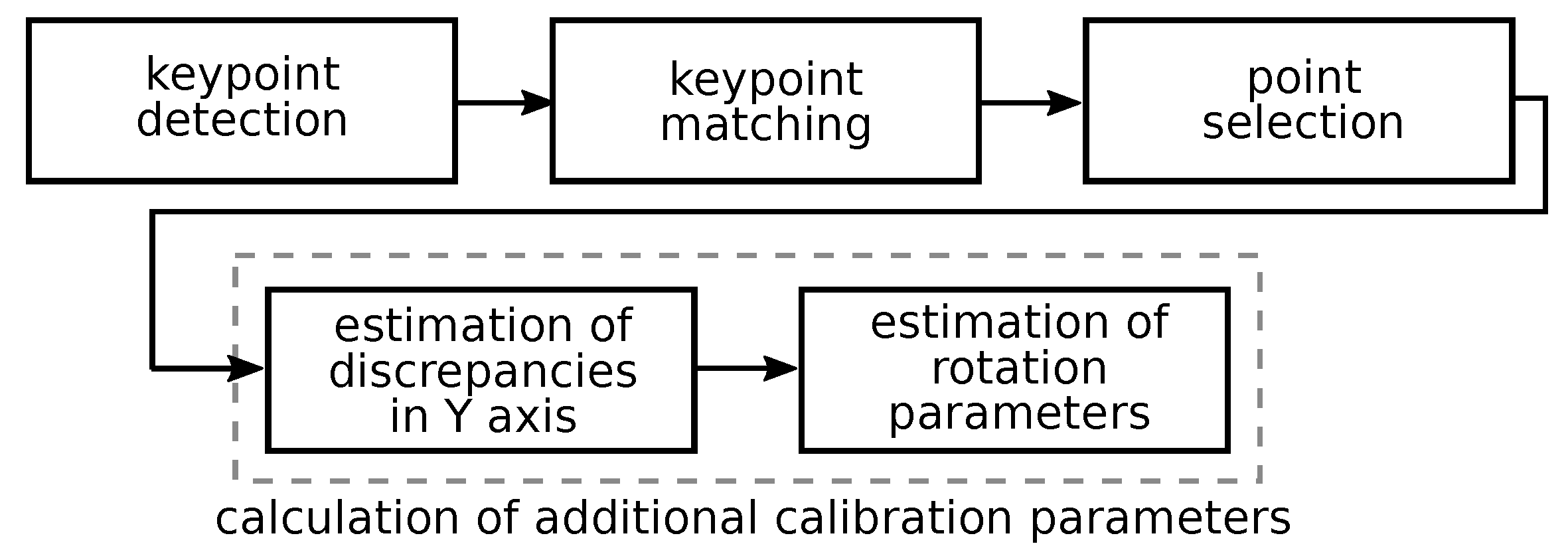
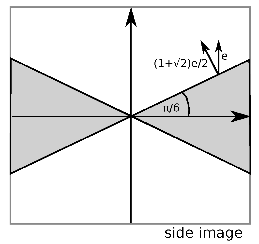
3.1. The Method of Auxiliary Calibration
Calculation of ACS Parameter
3.2. Test Data
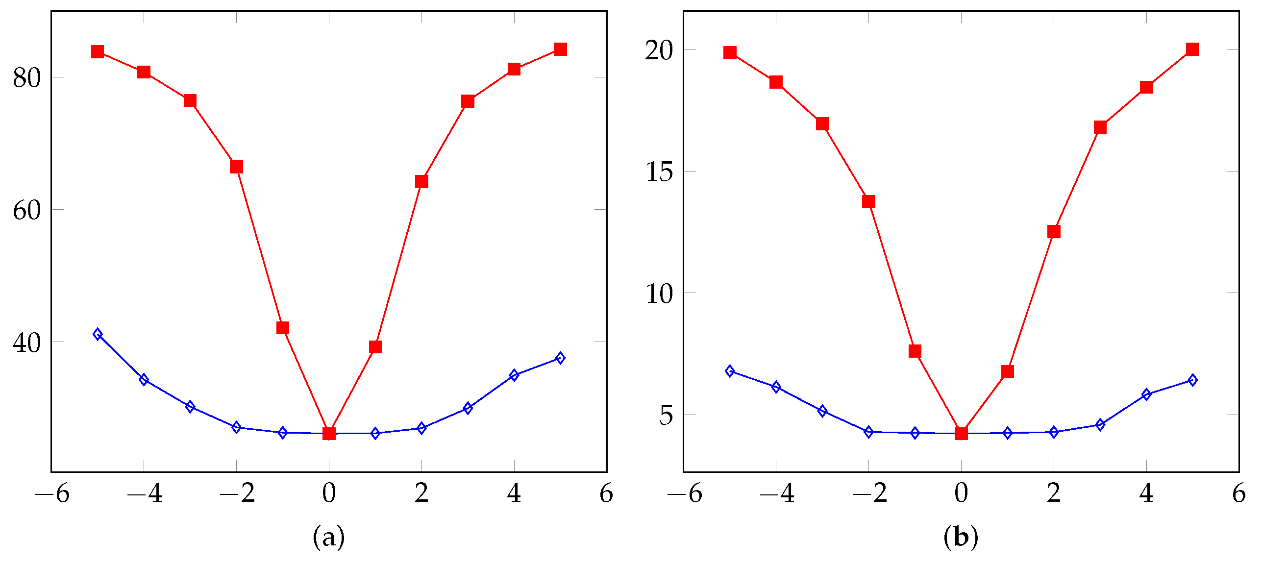
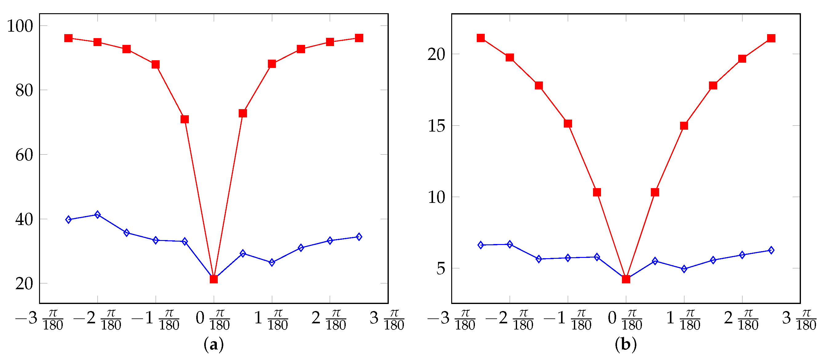
4. Results
5. Conclusions
Funding
Institutional Review Board Statement
Informed Consent Statement
Data Availability Statement
Conflicts of Interest
Abbreviations
| LIDAR | Light Detection and Ranging |
| ELAS | Efficient Large-scale Stereo Matching |
| StereoSGBM | Stereo Semi-Global Block Matching |
| BMP | Percentage of bad matching pixels |
| ACS | Auxiliary calibration step |
| SIFT | Scale-invariant feature transform |
| SURFs | Speeded up robust features |
References
- Scharstein, D.; Szeliski, R. A Taxonomy and Evaluation of Dense Two-Frame Stereo Correspondence Algorithms. Int. J. Comput. Vis. 2002, 47, 7–42. [Google Scholar] [CrossRef]
- Geiger, A.; Lenz, P.; Urtasun, R. Are we ready for autonomous driving? The KITTI vision benchmark suite. In Proceedings of the 2012 IEEE Conference on Computer Vision and Pattern Recognition, Providence, RI, USA, 16–21 June 2012; pp. 3354–3361. [Google Scholar] [CrossRef]
- Middlebury Stereo Evaluation—Version 3. Available online: https://vision.middlebury.edu/stereo/eval3/ (accessed on 23 August 2024).
- KITTI Vision Benchmark Suite. Available online: https://www.cvlibs.net/datasets/kitti/ (accessed on 23 August 2024).
- Geiger, A.; Roser, M.; Urtasun, R. Efficient Large-Scale Stereo Matching. In Computer Vision—ACCV 2010, Proceedings of the 10th Asian Conference on Computer Vision, Queenstown, New Zealand, 8–12 November 2010, Revised Selected Papers, Part I; Kimmel, R., Klette, R., Sugimoto, A., Eds.; Lecture Notes in Computer Science (LNCS, Volume 6492); Springer: Berlin/Heidelberg, Germany, 2011; pp. 25–38. [Google Scholar] [CrossRef]
- Bradski, D.G.R.; Kaehler, A. Learning Opencv, 1st ed.; O’Reilly Media, Inc.: Sebastopol, CA, USA, 2008. [Google Scholar]
- Georgopoulos, A.; Ioannidis, C.; Valanis, A. Assessing the performance of a structured light scanner. Int. Arch. Photogramm. Remote Sens. Spat. Inf. Sci. 2010, 38, 251–255. [Google Scholar]
- Roriz, R.; Cabral, J.; Gomes, T. Automotive LiDAR Technology: A Survey. IEEE Trans. Intell. Transp. Syst. 2022, 23, 6282–6297. [Google Scholar] [CrossRef]
- Seitz, S.M.; Curless, B.; Diebel, J.; Scharstein, D.; Szeliski, R. A Comparison and Evaluation of Multi-View Stereo Reconstruction Algorithms. In Proceedings of the 2006 IEEE Computer Society Conference on Computer Vision and Pattern Recognition (CVPR’06), New York, NY, USA, 17–22 June 2006; Volume 1, pp. 519–528. [Google Scholar] [CrossRef]
- 19 LiDAR Sensor Manufacturers in 2025. Available online: https://us.metoree.com/categories/lidar/ (accessed on 24 March 2025).
- StereoLab Store. Available online: https://www.stereolabs.com/en-pl/store (accessed on 24 March 2025).
- Basler Stereo Cameras. Available online: https://www.baslerweb.com/en/cameras/basler-stereo-camera/?utm_source=google&utm_medium=cpc&utm_campaign=EU+EN+-+NB+-+Prio+1&utm_term=NB+-+Stereo&utm_id=6809394628&gad_source=1&gclid=Cj0KCQjwhYS_BhD2ARIsAJTMMQa__kfTw8d2B4iB83TrfKFPa-EBL6t5CXD3PoNiG3jGzqW923IHpekaAoH-EALw_wcB (accessed on 24 March 2025).
- Stereoscopic Photography with StereoPi and a Raspberry Pi. Available online: https://www.raspberrypi.com/news/stereoscopic-photography-stereopi-raspberry-pi/ (accessed on 24 March 2025).
- Geiger, A.; Lenz, P.; Stiller, C.; Urtasun, R. Vision meets Robotics: The KITTI Dataset. Int. J. Robot. Res. 2013, 32, 1231–1237. [Google Scholar]
- Moravec, J.; Šára, R. High-recall calibration monitoring for stereo cameras. Pattern Anal. Appl. 2024, 27, 41. [Google Scholar] [CrossRef]
- Zhang, Z. A flexible new technique for camera calibration. IEEE Trans. Pattern Anal. Mach. Intell. 2000, 22, 1330–1334. [Google Scholar] [CrossRef]
- Triggs, B.; McLauchlan, P.F.; Hartley, R.I.; Fitzgibbon, A.W. Bundle Adjustment—A Modern Synthesis. In Vision Algorithms: Theory and Practice, Proceedings of the International Workshop on Vision Algorithms, Corfu, Greece, 21–22 September 1999; Triggs, B., Zisserman, A., Szeliski, R., Eds.; Springer: Berlin/Heidelberg, Germany, 2000; pp. 298–372. [Google Scholar]
- Camera Calibration and 3D Reconstruction. Available online: https://docs.opencv.org/4.x/d9/d0c/group__calib3d.html (accessed on 24 March 2025).
- Geiger, A.; Moosmann, F.; Car, O.; Schuster, B. Automatic Calibration of Range and Camera Sensors using a single Shot. In Proceedings of the 2012 IEEE International Conference on Robotics and Automation, Saint Paul, MN, USA, 14–18 May 2012. [Google Scholar]
- Li, B.; Heng, L.; Koser, K.; Pollefeys, M. A multiple-camera system calibration toolbox using a feature descriptor-based calibration pattern. In Proceedings of the 2013 IEEE/RSJ International Conference on Intelligent Robots and Systems, Tokyo, Japan, 3–7 November 2013; pp. 1301–1307. [Google Scholar] [CrossRef]
- Duan, Q.; Wang, Z.; Huang, J.; Xing, C.; Li, Z.; Qi, M.; Gao, J.; Ai, S. A deep-learning based high-accuracy camera calibration method for large-scale scene. Precis. Eng. 2024, 88, 464–474. [Google Scholar] [CrossRef]
- Hartley, R.I.; Zisserman, A. Multiple View Geometry in Computer Vision, 2nd ed.; Cambridge University Press: Cambridge, UK, 2004; ISBN 0521540518. [Google Scholar]
- Li, H.; Yin, J.; Jiao, L. Digital Surface Model Generation from Satellite Images Based on Double-Penalty Bundle Adjustment Optimization. Appl. Sci. 2024, 14, 7777. [Google Scholar] [CrossRef]
- Li, H.; Yin, J.; Jiao, L. An Improved 3D Reconstruction Method for Satellite Images Based on Generative Adversarial Network Image Enhancement. Appl. Sci. 2024, 14, 7177. [Google Scholar] [CrossRef]
- Bay, H.; Ess, A.; Tuytelaars, T.; Gool, L.V. Speeded-Up Robust Features (SURF). Comput. Vis. Image Underst. 2008, 110, 346–359. [Google Scholar] [CrossRef]
- Hosseininaveh, A.; Serpico, M.; Robson, S.; Hess, M.; Boehm, J.; Pridden, I.; Amati, G. Automatic Image Selection in Photogrammetric Multi-view Stereo Methods. In Proceedings of the 13th International Symposium on Virtual Reality, Archaeology and Cultural Heritage VAST, Brighton, UK, 19–21 November 2012; pp. 9–16. [Google Scholar]
- Scharstein, D.; Hirschmüller, H.; Kitajima, Y.; Krathwohl, G.; Nešić, N.; Wang, X.; Westling, P. High-Resolution Stereo Datasets with Subpixel-Accurate Ground Truth. In Pattern Recognition, Proceedings of the 36th German Conference, GCPR 2014, Münster, Germany, 2–5 September 2014; Jiang, X., Hornegger, J., Koch, R., Eds.; Springer: Cham, Switzerland, 2014; pp. 31–42. [Google Scholar]
- Kaczmarek, A.L.; Blaschitz, B. Equal Baseline Camera Array—Calibration, Testbed and Applications. Appl. Sci. 2021, 11, 8464. [Google Scholar] [CrossRef]
- Zhang, S.; Liu, S.; Ma, Y.; Qi, C.; Ma, H.; Yang, H. Self calibration of the stereo vision system of the Chang’e-3 lunar rover based on the bundle block adjustment. ISPRS J. Photogramm. Remote Sens. 2017, 128, 287–297. [Google Scholar] [CrossRef]
- Yang, B.; Pi, Y.; Li, X.; Yang, Y. Integrated geometric self-calibration of stereo cameras onboard the ZiYuan-3 satellite. ISPRS J. Photogramm. Remote Sens. 2020, 162, 173–183. [Google Scholar] [CrossRef]
- Liu, R.; Zhang, H.; Liu, M.; Xia, X.; Hu, T. Stereo Cameras Self-Calibration Based on SIFT. In Proceedings of the 2009 International Conference on Measuring Technology and Mechatronics Automation, Zhangjiajie, China, 11–12 April 2009; Volume 1, pp. 352–355. [Google Scholar] [CrossRef]
- Boukamcha, H.; Atri, M.; Smach, F. Robust auto calibration technique for stereo camera. In Proceedings of the 2017 International Conference on Engineering MIS (ICEMIS), Monastir, Tunisia, 8–10 May 2017; pp. 1–6. [Google Scholar] [CrossRef]
- Yin, H.; Ma, Z.; Zhong, M.; Wu, K.; Wei, Y.; Guo, J.; Huang, B. SLAM-Based Self-Calibration of a Binocular Stereo Vision Rig in Real-Time. Sensors 2020, 20, 621. [Google Scholar] [CrossRef] [PubMed]
- Hirschmüller, H. Stereo Processing by Semiglobal Matching and Mutual Information. IEEE Trans. Pattern Anal. Mach. Intell. 2008, 30, 328–341. [Google Scholar] [CrossRef] [PubMed]
- Scharstein, D.; Szeliski, R. High-accuracy stereo depth maps using structured light. In Proceedings of the 2003 IEEE Computer Society Conference on Computer Vision and Pattern Recognition, 2003. Proceedings, Madison, WI, USA, 18–20 June 2003; Volume 1, pp. 195–202. [Google Scholar] [CrossRef]
- Scharstein, D.; Pal, C. Learning Conditional Random Fields for Stereo. In Proceedings of the 2007 IEEE Conference on Computer Vision and Pattern Recognition, Minneapolis, MN, USA, 17–22 June 2007; pp. 1–8. [Google Scholar] [CrossRef]
- Hirschmuller, H.; Scharstein, D. Evaluation of Cost Functions for Stereo Matching. In Proceedings of the 2007 IEEE Conference on Computer Vision and Pattern Recognition, Minneapolis, MN, USA, 17–22 June 2007; pp. 1–8. [Google Scholar] [CrossRef]
- Khan, N.Y.; McCane, B.; Wyvill, G. SIFT and SURF Performance Evaluation against Various Image Deformations on Benchmark Dataset. In Proceedings of the 2011 International Conference on Digital Image Computing: Techniques and Applications, Noosa, Australia, 6–8 December 2011; pp. 501–506. [Google Scholar] [CrossRef]
- Drews, P.; de Bem, R.; de Melo, A. Analyzing and exploring feature detectors in images. In Proceedings of the 2011 9th IEEE International Conference on Industrial Informatics, Lisbon, Portugal, 26–29 July 2011; pp. 305–310. [Google Scholar] [CrossRef]

Disclaimer/Publisher’s Note: The statements, opinions and data contained in all publications are solely those of the individual author(s) and contributor(s) and not of MDPI and/or the editor(s). MDPI and/or the editor(s) disclaim responsibility for any injury to people or property resulting from any ideas, methods, instructions or products referred to in the content. |
© 2025 by the author. Licensee MDPI, Basel, Switzerland. This article is an open access article distributed under the terms and conditions of the Creative Commons Attribution (CC BY) license (https://creativecommons.org/licenses/by/4.0/).
Share and Cite
Kaczmarek, A.L. A Method for Adapting Stereo Matching Algorithms to Real Environments. Appl. Sci. 2025, 15, 4070. https://doi.org/10.3390/app15074070
Kaczmarek AL. A Method for Adapting Stereo Matching Algorithms to Real Environments. Applied Sciences. 2025; 15(7):4070. https://doi.org/10.3390/app15074070
Chicago/Turabian StyleKaczmarek, Adam L. 2025. "A Method for Adapting Stereo Matching Algorithms to Real Environments" Applied Sciences 15, no. 7: 4070. https://doi.org/10.3390/app15074070
APA StyleKaczmarek, A. L. (2025). A Method for Adapting Stereo Matching Algorithms to Real Environments. Applied Sciences, 15(7), 4070. https://doi.org/10.3390/app15074070