Abstract
Hollow wear on wheels is a common form of surface damage often observed in high-velocity vehicles. It is widely recognized that hollow wear of the wheel tread degrades the dynamic performance of rail vehicles, especially in the issue commonly referred to as “operational stability”, and leads to abnormal wheel–rail contact interactions. However, the evaluation criteria for vehicle stability are not uniform, which affects the assessment of wheel conditions and the timing of wheel re-profiling during maintenance. Therefore, numerical simulations were conducted by matching the measured worn wheel profiles with standard rails, and three different methods were employed to evaluate vehicle stability in this article. The numerical results revealed that the wheel equivalent conicity exhibits a nonlinear characteristic caused by hollow wear, which means that the nominal equivalent conicity is unable to accurately represent the geometric contact relationship between the wheel and rail. Under identical wheel wear conditions, a certain difference was observed in the critical speed of the vehicle determined by the velocity-reducing method and the bifurcation configuration method. Both methods were capable of reflecting the impact of wheel hollow wear on vehicle stability at the critical speed. Compared to the velocity-reducing method, the bifurcation configuration method can better reflect the transition process of a vehicle from stable running to hunting instability. Furthermore, the lateral vibration acceleration values measured above the bogie frame indicated that slight wheel wear is insensitive to increased speed. However, when the wear was severe, the lateral vibration acceleration of the bogie was found to increase sharply, exceeding the established stability criteria. This phenomenon was consistent with the safety alarms that occurred during actual vehicle operation, indicating that the vehicle had failed to meet stability requirements.
1. Introduction
The stability, safety, and comfort of the vehicle are crucial for the operation of railways as an efficient mode of transportation. Under high-speed, heavy-load, and long-term service conditions, the wear of wheel tread continuously intensifies. As the vehicle travel distance increases, lateral acceleration alarms on the bogies occur frequently during operation. Through maintenance of the vehicle, it is found that the wheels that reported the alarm exhibit varying degrees of hollow wear.
Hollow wear primarily occurs in the vicinity of the nominal rolling circle on the tread of the wheel. This phenomenon is commonly observed in high-speed trains and subways, attributed to the significant curvature radius of the railway and the high flatness of the rails. Sawley [1,2] conducted a comprehensive survey of wheel profiles for over 6700 wheels across a wide range of freight vehicles operating in North American freight railways. The survey revealed that a significant proportion of these wheels exhibited hollow wear shapes, and 45.5% of the wheels had hollow wear less than 0.25 mm, while 6.2% had wear exceeding 3 mm. Dynamic analysis further demonstrated that such hollow wheel shapes impair the steering ability of bogies, leading to increased rolling resistance and higher lateral forces between the wheels and rails. Zhai [3] monitored a certain number of EMUs in China over a certain period. The wheel wear data indicated that 69.29% of the wheels displayed hollow wear surpassing a depth of 0.2 mm. The lateral axle box acceleration spectra measured above the wheels indicated that, compared with new wheels, wheels with hollow wear had much higher amplitudes in the frequency range of 6–9 Hz. Tavakkoli [4] developed a multibody dynamic model for the vehicle and examined how the instability was affected by the ‘false wheel flange’ resulting from hollow wear. Hollow wear not only affects the lateral stability of the vehicle, but also increases the stress in the contact area between the false flange of the wheel and rail, exacerbating rolling contact fatigue and plastic deformation of the wheel rail material [3,5]. Alizadeh Kaklar [6] explored how hollow wear influences the variability and vibrations experienced by a wagon, taking into account the importance of both single- and dual-point wheel–rail contact as key factors. Particularly, the presence of a hollow design resembling a false flange greatly enhances the extent of lateral movement in the wheelset, while erosion at the base of the wheel flange amplifies this problem. The above research indicates that different types of railway vehicles generally have hollow wear on the wheel tread after long-term operation, but the depth of hollow wear is different. Moreover, the impact of hollow wear on vehicle stability is not fixed, and is influenced by various factors such as railway environment, vehicle speed, and suspension system parameters. Considering the operating cost of railways, a certain level of hollow wear is allowed. However, once the wear reaches the specified threshold, it is necessary to repair the wheel profile through mechanical processing. In general, for low-speed wagons, a larger range of hollow wear values may be allowed, but high-speed EMUs are more sensitive to the wheels’ geometric deviations than freight wagons. Therefore, hollow wear has a greater impact on the stability of vehicles at high speeds.
The methods and standards for judging vehicle stability are not uniform. Zhai [7] revealed the characteristics of the lateral acceleration value or frequency spectrum of the bogie axle box through numerical simulation and actual testing. By measuring the vertical and lateral forces between the wheel and rail, the lateral force of the wheel axle, derailment coefficient, wheel load reduction rate, and other indicators, calculations can be performed to intuitively evaluate the stability of the vehicle [8,9]. In addition, because of the nonlinear interaction between the wheel and the rail, it is possible for Hopf bifurcation and limit cycle motion to take place while the wheelset is in motion. So, the bifurcation configuration method can also be used to evaluate the stability of vehicles [10,11]. Polach [12,13] presented a computation of bifurcation diagram and the influence of nonlinearities of the vehicle system on the type of Hopf bifurcation investigated. For a detailed model of a railway passenger coach, he used two different methods to analyze the oscillation behavior depending on operating speed, wheel–rail contact conditions, and different model configurations. Li [14] studied the influence of different nonlinear equivalent conicity functions on bifurcation characteristics. Lei [15] used the root locus method to calculate the natural vibration frequency and natural damping of each rigid body in the vehicle system at different operating speeds. This method is a linear frequency domain calculation method, where different trajectory lines represent the natural frequency changes of different rigid bodies in the calculation model at different speeds. When the natural damping coefficient of a certain root locus is less than 0, it indicates that the system has become unstable. Due to the neglect of the influence of nonlinear factors in the system, the calculated critical speed value of the vehicle is relatively high, and this article will not continue to discuss the root locus method. Compared to other methods, the velocity-reducing method is simpler. By establishing a vehicle–track dynamics model, the convergence of lateral vibration of wheelsets can be simulated, thereby the critical speed of the vehicle instability can be calculated [16]. In the vehicle design, improvement, and maintenance processes, the velocity-reducing method, bifurcation configuration method, and measurement of lateral acceleration of the bogie frame have been widely used to assess vehicle stability. However, previous studies have not focused on whether the stability assessment results obtained from these three methods are consistent and the differences among them. To investigate the impact of hollow wear on vehicle stability, the measured worn wheel profiles were matched with standard rails, and dynamic simulations were conducted using these methods under identical wheel hollow wear conditions in this study. In addition, the characteristics of these methods were elucidated. The insights are expected to inform more effective maintenance strategies and safety assessments for high-speed rail vehicles.
2. The Influence of Tread Hollow Wear on the Wheel–Rail Contact Relationship
2.1. The Profile of Worn Wheels
Characterizing hollow wear solely by its depth has certain limitations. In fact, hollow wear on the wheel tread is not only related to the depth and width of the wear, but also closely associated with the position of the hollow wear. For hollow wear of wheel tread (as in Figure 1), the wear depth H is defined as the radius difference between the standard and worn wheel profiles at a point 70 mm from the flange’s back. However, this position is not the deepest point of hollow wear. Point A is defined as the highest point on the outer side of the wheel wear profile (away from the flange), Point B is the lowest point of the hollow wear, and the vertical distance h between A and B is the depth of hollow wear. The investigation showed that a hollow wear depth between 0.1 mm and 0.3 mm can easily lead to frame lateral acceleration exceeding the limit, triggering safety alarms and necessitating vehicle deceleration or halt [3].
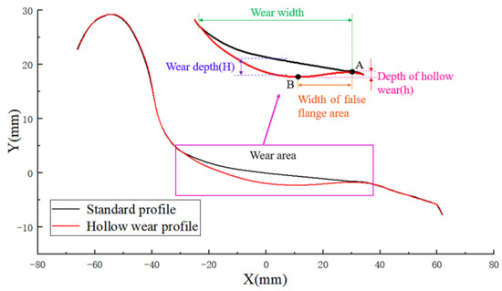
Figure 1.
The wheel hollow wear.
It is well understood that the hollow wear in wheel treads intensifies as mileage increases. To study the wheel–rail contact situation of worn wheel, a wheel profile measuring instrument was used to measure the tread profile of a selected wheelset of the high-speed train during one maintenance cycle, as shown in Figure 2.
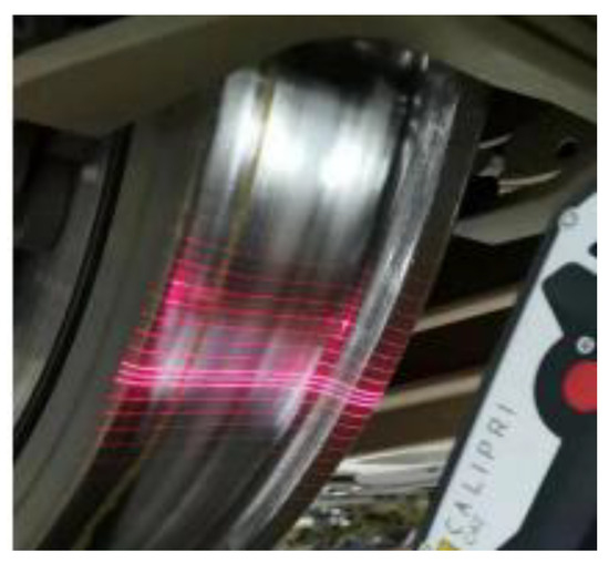
Figure 2.
Field measurements for wheel profile.
The standard wheel tread profile (which had been re-profiled) was defined as W1. Corresponding to different operating mileage of the vehicle (45,000 km, 95,000 km, 185,000 km, and 260,000 km), the profiles of worn wheel were labeled as W2~W5, respectively. The main parameters characterizing the hollow wear are listed in Table 1, as the calculation basis for subsequent analysis of wheel–rail contact point evolution and dynamic simulation. The data show that with the increase in mileage, the depth and width of wear on the wheel tread progressively rise, and the profile of wheel undergoes a dynamic development process.

Table 1.
Measurement results of wheel wear profiles in a re-profiling interval.
2.2. Dynamic Model
To study the effect of hollow wear on the dynamics of high-speed vehicles, the dynamics model was developed using multibody system software SIMPACK 2018 (as shown in Figure 3). The model was established for a single vehicle, ignoring the asymmetry of the vehicle structure and loading, as well as the nonlinear factors between connecting components. Therefore, it may be simplified to a multi-degree-of-freedom system consisting of the vehicle body, frame, and wheelsets, with each component connected by linear springs and damping units. The relative motion of the vehicle system is shown in Table 2.
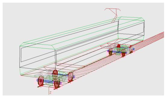
Figure 3.
The dynamics model.
Table 2.
The relative motion of the vehicle system.
The vehicle model comprises a single carbody, a pair of bogie frames, four wheelsets, and associated gearboxes. Its primary suspension system features a steel spring, a vertical shock absorber, and a module for positioning the axle box arm. The secondary suspension is equipped with an air spring, an anti-roll torsion bar, a lateral shock absorber as well as both vertical and anti-hunting shock absorbers, in addition to a lateral stop. Key parameters of the vehicle are shown in Table 3.
Table 3.
The main parameters of a single vehicle.
The calculation is based on full load conditions, utilizing a 60N rail and an LMC tread wheel. The gauge of the rail measures 1435 mm, with a cant of 1:40. Additionally, the inner spacing between the wheelset is 1353 mm. There is a certain deviation between the actual position and the ideal position of the rail on the railway line, which is called track irregularity and is the primary contributor to vibrations within vehicle systems. The spectrum of track irregularity measured along the Beijing Tianjin line in China (as shown in Figure 4) is used for the track excitation in SIMPACK software.
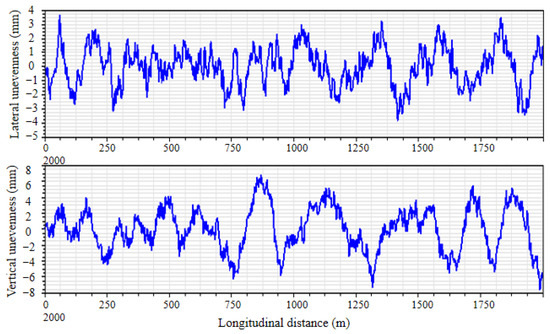
Figure 4.
The track irregularity spectrum.
2.3. Distribution of Wheel–Rail Contact Points
Using to the data in Table 1, the study employed a contact algorithm to calculate the wheel–rail contact geometry relationship between a worn wheel and a 60N rail. The wheel moved laterally from the center position, and the distribution of wheel–rail contact points under different lateral displacements were obtained. Without considering the shaking motion and elastic deformation of the wheelset, the wheel–rail contact geometry relationship of the worn tread under different operating mileage is shown in Figure 5.
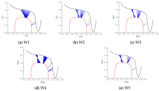
Figure 5.
Wheel–rail contact geometry evolutions.
The observation reveals that when the new wheel profile (W1) aligns with the new CHN60 profile, the allocation of wheel–rail contact points on the tread becomes concentrated. In this scenario, the distribution of wheel–rail contact points on the side of the wheel flange is sparse and evenly spread, which is an ideal one-point contact situation. As the train travel distance increases, for the worn wheels W2~W5, the worn wheel–rail contact points gradually spread towards both sides of the wear areas due to the intensification of wear depth and width. Moreover, the wheel–rail contact point jumps between various equilibrium positions, thereby generating impact vibrations associated with the “false flange” [17]. This indicates that the hollow wear on the wheel significantly alters the condition of wheel–rail contact, leading to a highly scattered and uneven arrangement of contact points between the wheel and rail. In such extreme conditions, the occurrence of two-point contact between the wheel and rail becomes quite common. It is important to highlight that both two-point and multipoint contact behaviors can exacerbate the interaction between the wheel and rail, thereby escalating the wear and deterioration of the profiles of both the wheel and rail [18,19].
2.4. Nonlinear Characteristics and Revised Equivalent Conicity for Worn Wheels
The nominal equivalent conicity is commonly used to characterize the wheel–rail contact geometry, and this method is only applicable for uniform wear but not for hollow wear. In fact, due to hollow wear on the wheel tread, the equivalent conicity decreases from the outer side towards the flange and then gradually increases. The equivalent conicity values under varying lateral displacements exhibit nonlinear characteristics. As a result, the nominal equivalent conicity cannot accurately reflect the wheel–rail geometric contact relationship of the tread.
The equivalent conicity values on multiple wheelsets of a certain type of high-speed train on the Ha-Da high-speed railway line were measured, and four wheels were selected and marked as A, B, C, D. The equivalent conicity curves are shown in Figure 6, characterized by the same equivalent conicity for 3 mm amplitude, but different values for other wheelset amplitudes.
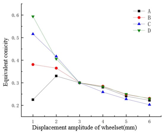
Figure 6.
Different equivalent conicity curves.
In response to this issue, Polach [20] considered the nonlinear characteristics of the equivalent conicity curve and expressed the equivalent conicity at point N on the wheel tread as follows:
According to the UIC 518 [21], when evaluating conicity values for wheelsets, it is essential to analyze the conicity values associated with amplitudes of 2 mm and 4 mm alongside the conicity value for an amplitude of 3 mm. By examining these three specific conicity values collectively, it becomes possible to establish a more comprehensive understanding of the conicity function. This approach allows for the calculation of a nonlinear parameter that characterizes how the conicity function changes in response to an increase in wheelset amplitude of 1 mm, specifically within the range of amplitudes from 2 mm to 4 mm. However, the lateral displacement of the wheelset increases under the poor railway line conditions, making it essential to broaden the equivalent conicity range. On this condition, the equivalent conicity can be revised as follows:
① By calculating the equivalent conicity values corresponding to the integer lateral displacements of the wheelset within the 1–6 mm range, the standard deviation is expressed as Equation (2)
where represents the equivalent conicity values for i = 1, 2,..., 6, and represents the average of these equivalent conicity values. A small standard deviation indicates that the equivalent conicity curve changes less.
② A nonlinear factor for the equivalent conicity curve was proposed, and it was defined as
③ The nonlinear factor was subtracted from the original nominal equivalent conicity value, after which the nonlinear equivalent conicity was revised.
To elucidate the impact of hollow wear on equivalent conicity, five types of wheels were matched with standard profile rail. The equivalent conicity curves, generated under various lateral displacements of the wheelset, are presented in Figure 7. The simulation results also showed that as the train travel distance increased, the average equivalent conicity value increased, and the equivalent conicity curve gradually showed a negative slope and nonlinear characteristics, further proving that the nonlinear equivalent conicity can more accurately reflect the differences in the transformation of the wheel–rail contact relationship than the nominal equivalent conicity.
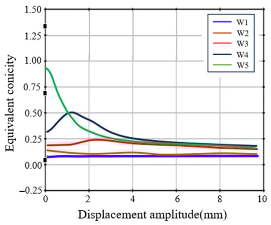
Figure 7.
Equivalent conicity curves of each wheel tread.
3. Impact of Hollow Worn Wheel on Vehicle Stability
3.1. Evaluation of Vehicle Stability Using Velocity-Reducing Method
In order to determine the critical speed of the vehicle under various hollow wear conditions, the five different profile wheels in Table 1 were further studied, using SIMPACK software to conduct simulation analyses on the vehicle system. Initially, the vehicle’s initial speed is set to a relatively high value. Excitations are then applied to the track, followed by the application of longitudinal forces to decelerate the vehicle. Through integration calculations, the lateral displacement of the wheelset is recorded over time. Based on the relationship curve between the lateral displacement of the wheelset and the vehicle’s traveling speed, the vehicle speed corresponding to the point where the lateral displacement of the wheelset gradually decays to the equilibrium position is identified. This is a process to obtain the critical speed of a vehicle using the velocity-reducing method.
The findings from the simulation demonstrate that there is a decrease in the vehicle’s critical speed as the hollow wear increases, as depicted in Figure 8. With the operational speed range for EMUs being 200–250 km/h, the allowable upper limit is established at 275 km/h, incorporating a 10% safety buffer. Nonetheless, the critical speeds for the vehicle associated with wheels W4 and W5 fall below this designated maximum speed. Consequently, when the vehicle reaches speeds above 265 km/h, the vibration amplitude of the wheelset stops converging and begins to escalate instead. This occurrence is referred to as hunting instability.
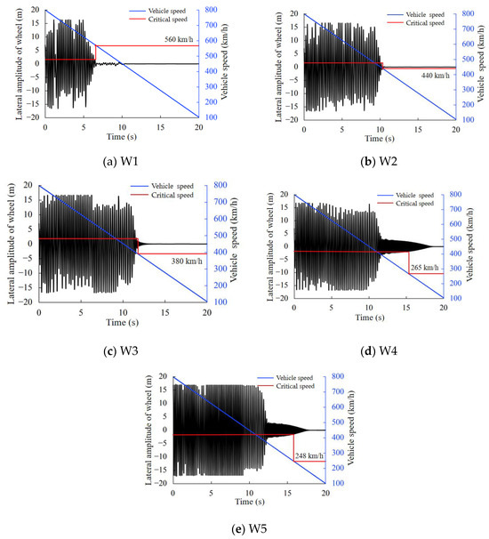
Figure 8.
Nonlinear critical speed corresponding to different worn wheels.
3.2. Evaluation of Vehicle Stability Using Bifurcation Configuration Method
3.2.1. Critical Speed and Bifurcation Type of Vehicles
Due to the nonlinear contact relationship between wheels and rails, bifurcation phenomena may occur during the movement of wheelsets, commonly represented by bifurcation diagrams.
According to the degrees of freedom listed in Table 2 and the motion differential equations of the vehicle system [22], let
Then, the nonlinear ordinary differential equation can be described the vehicle’s dynamic behavior by reducing the order.
where is called the control parameter or bifurcation parameter [23], and . In this article, the vehicle operating speed was used as the bifurcation parameter of the system, and the equilibrium solution of the nonlinear differential equation satisfied the following equation:
As the velocity of the vehicle rises, the complex conjugate eigenvalues of the Jacobi matrix cross the imaginary axis, and the system exhibits Hopf bifurcation [24]. Meanwhile, the equilibrium solution for the vehicle system transitions from a stable state to an unstable state.
Therefore, in the stability analysis of the vehicle system, the bifurcation diagram illustrates the amplitude of the limit cycle (often represented by the lateral displacement of the wheelset) as a function of the vehicle’s speed. The commonly used numerical calculation methods for solving limit cycles include the direct integration method, shooting method, and continuation algorithm. In this study, the shooting method is applied to solve the bifurcation configuration diagram of vehicles.
The bifurcation configuration of vehicles traveling in a straight line usually has three main forms, as shown in Figure 9. Figure 9a shows subcritical bifurcation, while Figure 9b,c show supercritical bifurcation. In the figure, the solid line denotes the stable limit cycle, while the dashed line denotes the unstable limit cycle; Point A is the Hopf bifurcation point of the vehicle system, defined as the linear critical speed, which is denoted as V_lin; Point B is the minimum speed at which vehicle hunting occurs, which is the nonlinear critical speed of the vehicle system, which is denoted as V_nl. In addition, Point D represents the saddle point of stable and unstable limit cycles.
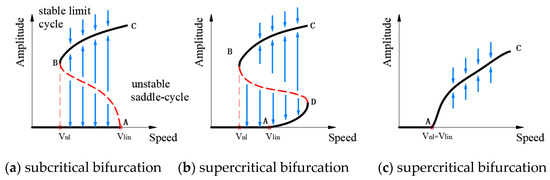
Figure 9.
Bifurcation diagram with subcritical and supercritical Hopf bifurcation.
In Figure 9a, when the vehicle’s speed is below the nonlinear critical speed (Point B), the limit cycle approaches zero irrespective of the initial excitation amplitude. However, once the vehicle’s speed surpasses this threshold, the amplitude of the limit cycle becomes contingent upon the initial excitation amplitude. If the initial excitation amplitude is within the AB line, the limit cycle converges to zero. If the initial excitation amplitude exceeds the amplitude corresponding to the AB line, the limit cycle will converge to the amplitude corresponding to the BC line. In Figure 9b, when the vehicle’s speed is greater than the nonlinear critical speed and the initial excitation amplitude exceeds the amplitude of the BD line, the limit cycle converges to the amplitude corresponding to the BC line, resulting in a larger amplitude of wheelset vibration. When the vehicle’ speed is between the BA point and the initial excitation amplitude is smaller than that of the BD line, the limit cycle converges to zero. When the vehicle speed is between the AD points and the initial excitation amplitude is smaller than the amplitude corresponding to the BD line, the corresponding limit cycle converges to the amplitude corresponding to the AD line, and the wheelset vibration amplitude is smaller. In Figure 9c, the linear and nonlinear critical speeds of the vehicle system are the same, both corresponding to Point A. When the vehicle’s speed exceeds this value, the limit cycle converges to the amplitude corresponding to the AC line.
3.2.2. Analysis of Hopf Bifurcation Diagram for Wheelsets
For vehicle dynamics systems, engineers focus on bifurcation speed points and bifurcation configurations, as the former relates to nonlinear critical speeds and the latter relates to the operational state of the vehicle after instability. Figure 10 shows the lateral vibration bifurcation configurations and corresponding nonlinear critical speeds for the five types of worn wheels with varying speeds, respectively. The speed of the vehicle is depicted on the horizontal axis, while the vertical axis illustrates the lateral vibration amplitude of the wheelset at various speeds. The threshold point of the limit cycle indicates the vehicle’s nonlinear critical speed.
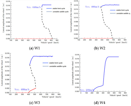
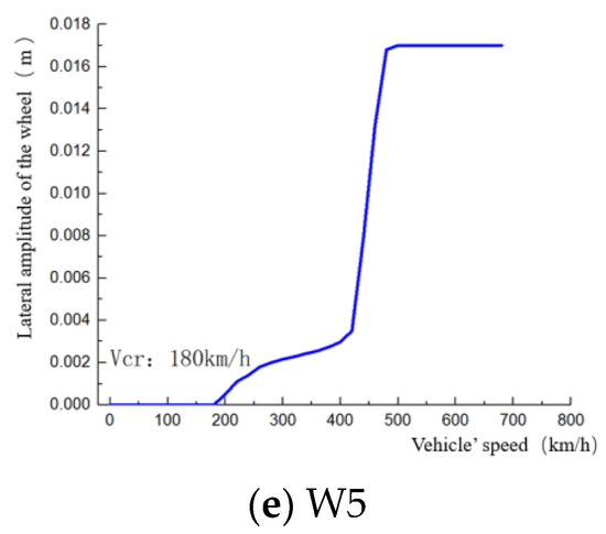
Figure 10.
Bifurcation configuration diagram of wheel’s lateral amplitude.
According to the lateral vibration limit cycle amplitude of standard profile wheel W1 and worn wheel W2, their bifurcation configurations are subcritical, as shown in Figure 10a,b, with corresponding nonlinear critical speeds of 640 km/h and 480 km/h, respectively. As the wheel wear intensifies, the bifurcation characteristics change from subcritical configuration to supercritical configuration, while the nonlinear critical speed decreases. As shown in Figure 10c, the operating mileage of the corresponding wheel is 95,000 km, and the nonlinear critical speed is 400 km/h, which already has the characteristics of a supercritical configuration. For the more severely worn wheels W4 and W5, the simulated nonlinear critical speed of the vehicle is reduced to 220 km/h and 180 km/h. Once the vehicle speed exceeds the nonlinear critical speed, the lateral displacement limit cycle amplitude of the wheelset cannot converge to zero, and the vehicle’s operational stability is significantly reduced. In this situation, it is unable to meet the requirement of a maximum operating speed of 250 km/h for a high-speed vehicle.
In addition, Figure 7 shows the equivalent conicity curves of each wheel tread. The equivalent conicity slopes of the tread surfaces of wheels W1 and W2 are positive at this position, which both have subcritical bifurcation configurations. The equivalent conicity slopes of the tread surfaces of wheels W3, W4, and W5 are negative at the corresponding positions, and the bifurcation configurations of these wheels are supercritical configurations. It can be inferred that there is a certain correlation between the slope of the equivalent conicity curve and the type of bifurcation configuration.
3.3. An Evaluation of Vehicle Stability Using the Lateral Vibration Acceleration Method
In order to monitor the safe operating status of vehicles, an alarm system is installed at the end of the bogie, and acceleration sensors are installed on the bogie frame that measures wheel–rail forces to provide a basis for speed limit processing. The acceleration of lateral vibration in the bogie frame is often utilized to assess the vehicle’s lateral stability.
As outlined in the Chinese national standard GB/T 5599-2019 [25], which details the criteria for evaluating dynamic performance and identifying tests for vehicles, real-time sampling of vibration acceleration above the axle box is carried out continuously within the maximum speed range during testing. Subsequently, the collected data undergo filtering using a band-pass filter set to a frequency range of 0.5 to 10 Hz. If the peak acceleration exceeds or reaches 8 m/s2 six consecutive times, it indicates that the continuous lateral vibration of the bogie cannot converge, thereby determining that the bogie is laterally unstable.
The maximum and average vibration accelerations at various speeds are derived from the lateral and vertical accelerations recorded at specific measurement points. Beyond these, the vehicle’s operational stability and safety are gauged through additional indicators. The vertical and lateral forces that interacted between the wheel and rail are ascertained using force-measuring wheels [26]. The dynamic performance of the vehicle is evaluated by assessing whether the lateral force on the wheel axle, the derailment coefficient, and the wheel load reduction rate conform to the requisite standards [27].
The force acting laterally on the axle of the wheel must adhere to Equation (8):
where and are the static load of the left and right wheels, respectively; is the peak value of the lateral force on the wheel axle.
The derailment coefficient should comply with
where Q is the lateral force exerted by the wheel at the climbing rail side on the rail, and P is the vertical force exerted by the wheel on the rail on the same side.
The wheel load reduction rate should comply with
where is the load reduction of the wheel, and is the average wheel load on the side where loading or unloading occurs.
The vehicle dynamics performance is shown in Figure 11 as the vehicle speed is gradually increased from 160 km/h to 300 km/h on a straight track, with a speed sampling step of 20 km/h. Figure 11a,b show the maximum vertical and lateral acceleration values of a carbody measured within this speed range. At the same speed, the difference in the maximum vertical acceleration among the five worn wheels is very small, but the difference in the maximum lateral acceleration is significant, especially for the worn wheels W4 and W5, which exhibit much greater lateral acceleration than the other wheels. This indicates that wheel hollow wear has a minor impact on the vertical vibration of the vehicle, but it has a significant effect on the lateral vibration.
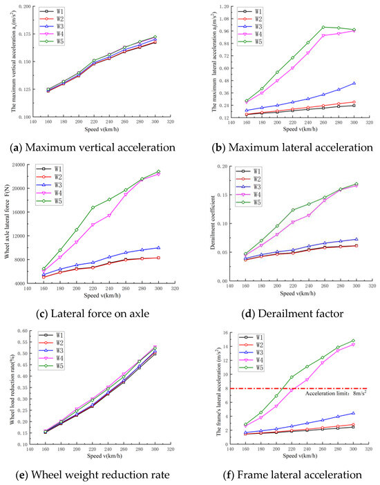
Figure 11.
Vehicle dynamics performance.
Figure 11c–e, respectively, depict the curves of wheel axle lateral force, derailment coefficient, and wheel load reduction rate as functions of speed for the five worn wheels. As the speed increases, the common characteristic of the wheel axle lateral force and derailment coefficient curves is that the slopes of the curves for worn wheels W4 and W5 are large, showing a significant difference from other tread surfaces. This indicates that once hollow wear reaches a certain depth, it significantly influences the lateral forces involved in the interaction between the wheel and rail. At the same time, the rate of wheel load reduction does not show a strong sensitivity to hollow wear, and no clear causal connection exists between the two.
The bogie frame, as the main body of the bogie, is constantly subjected to complex dynamic loads. When high-frequency vibrations generated by wheel–rail interactions are transmitted to the bogie frame through the primary suspension, a significant amount of energy remains. The variation of the lateral vibration acceleration of the bogie frame with speed, corresponding to different hollow wear profiles, is shown in Figure 11f. As the vehicle speed increases, the lateral vibration acceleration of the frame also gradually increases, with the curves of the severely worn wheels W4 and W5 showing a sharp increase in slope. When the speed of the vehicle hits 220 km/h, the W4 curve shows that the lateral acceleration of the bogie frame goes beyond the alarm threshold set at 8 m/s2.
However, the criterion for determining the lateral instability of the bogie is that the peak acceleration exceeds 8 m/s2 six or more consecutive times. The values depicted in Figure 11f fail to represent the variations in lateral acceleration of the bogie frame over time. Consequently, a time domain analysis of the lateral acceleration of the bogie frame was performed. As illustrated in Figure 12, at a speed of 250 km/h, the lateral vibration acceleration associated with W4 is markedly increased, while the lateral vibration acceleration related to W5 exceeds the acceptable limit on multiple occasions, indicating that the lateral stability of the vehicle does not fulfill the necessary criteria.
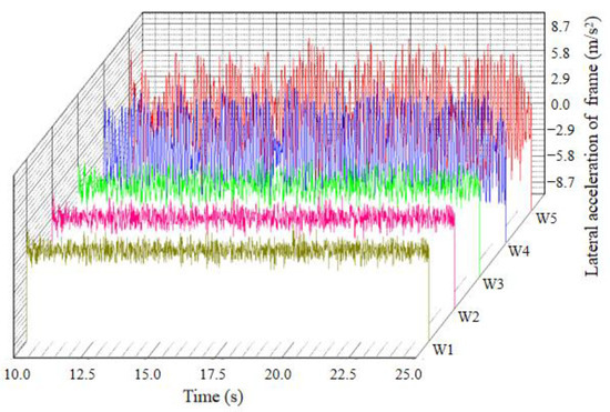
Figure 12.
Time domain diagram for lateral acceleration of bogie frame.
4. Experimental Analysis
To comprehend the vibration properties of high-speed trains functioning on real railway lines, measurements were taken during tracking and tests were performed on the vehicles. Firstly, acceleration sensors were installed under the carriage and above the steel springs of the longitudinal beam of the bogie frame (see Figure 13) to monitor the vibration acceleration of the vehicle body and bogie. At the same time, a portable wheel tread measuring instrument was used to obtain the profile of the wheel tread. The first measurement was taken when the vehicle had traveled 260,000 km, and the second measurement was taken after the wheels were re-profiled, corresponding to the profiles W5 and W1 in Table 1, respectively.
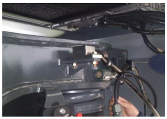
Figure 13.
Arrangements of vibration measuring sensors for bogie frame.
Figure 14 and Figure 15 present the results of testing the lateral acceleration response for both the vehicle body and the bogie. A comparative analysis reveals that the lateral acceleration recorded on the frame of the bogie is significantly greater than that observed in the vehicle body. This is because the vibration generated by the wheel–rail interaction is transmitted to the vehicle body through various damping elements of the bogie, ensuring the ride comfort of the vehicle body [28]. During the first test, the vehicle was approaching the maintenance cycle and the measured lateral vibration acceleration value of the bogie exceeded the instability alarm limit. The second measurement showed a significant decrease in the lateral vibration acceleration value of the bogie, indicating that the repaired high-speed train has better lateral stability and verifying the correctness of the simulation results.
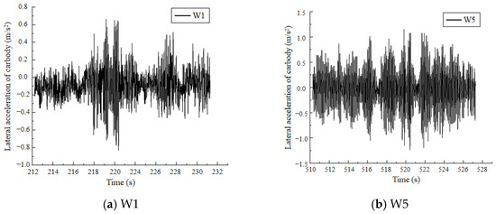
Figure 14.
The lateral acceleration of the carbody.
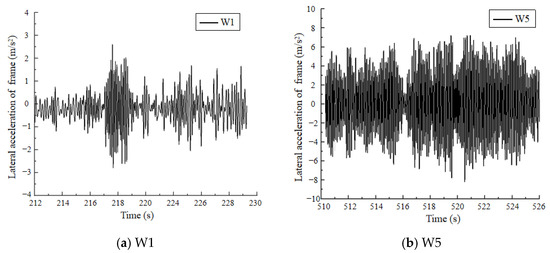
Figure 15.
The lateral acceleration of the frame.
5. Discussion
Based on the measured wheel profile, this paper examines how the hollow wear of wheels affects the geometric relationship between wheel–rail contact and the stability of the vehicle.
With an increase in the vehicle’s mileage, both the depth and width of the hollow wear intensifies, and the wheel equivalent conicity has nonlinear characteristics. And thus, the nominal equivalent conicity cannot accurately reflect the wheel–rail geometric contact relationship. It is more accurately depicted by using nonlinear equivalent conicity to reflect the contact relationship between worn wheel and rail.
The critical speeds corresponding to different degrees of wheel hollow wear were obtained using the velocity-reducing method and the bifurcation configuration method. These methods indirectly assess the vehicle’s stability by comparing the critical speeds with the vehicle’s actual operating speed. The numerical results show that under the same wheel wear conditions, there is a certain difference in the critical speeds determined by the two methods. The bifurcation configuration method better reflects the transition process of the vehicle from stable operation to hunting instability. In addition, through the dynamic simulation of the vehicle system, the maximum vertical and lateral accelerations of the carbody and the lateral vibration acceleration of the bogie frame can be obtained. The data indicate that wheel tread hollow wear has a relatively small effect on the vertical vibration of the carbody, but a significant effect on the lateral vibration. This is because the contact points between the wheel and rail gradually spread to both sides of the hollow wear area, leading to increased lateral impacts between the wheel and rail. Slight hollow wear is not sensitive to speed, but when the hollow wear is severe, the lateral vibration acceleration of the bogie increases sharply. The conclusions drawn from the three methods show that as hollow wear intensifies, the critical speed of the vehicle decreases or the lateral acceleration of the bogie exceeds the limit. They are commonly used in suspension system design, wheel profile improvement, and vehicle system performance analysis.
As the vehicle operates on the track, the sensors mounted on the body and bogie continuously capture the vibration acceleration data of both the body and frame in real time, allowing for intuitive monitoring of this information. The results from the simulation align with the actual functioning of the vehicle, demonstrating that hollow wear on the wheels considerably affects vehicle stability.
In response to the vibration issues caused by hollow wear, the current practice of railway maintenance departments is to restore the standard profile of wheels through re-profiling. In the future, as an additive manufacturing method, the application of laser cladding technology in repairing hollow wear damage deserves further research.
Author Contributions
Conceptualization, L.Z. and J.H.; methodology, L.Z.; software, C.W.; validation, L.Z. and J.H.; formal analysis L.Z.; investigation, C.W.; resources, Z.L.; data curation, L.Z.; writing—original draft preparation, L.Z.; writing—review and editing, L.Z.; visualization, C.W.; supervision, J.H.; project administration, J.H. All authors have read and agreed to the published version of the manuscript.
Funding
This research was funded by the National Natural Science Foundation of China (Grant No. 12393783), the Research and Development Project of Science and Technology of China Railway Corporation (N2023T011-B(JB)), and the Natural Science Foundation of Hunan Province (Grant No. 2021JJ40181).
Acknowledgments
We would like to acknowledge the Central South University for providing the research facilities and laboratory space necessary for this study.
Conflicts of Interest
The authors declare no conflict of interest.
References
- Sawley, K.; Wu, H. The formation of hollow-worn wheels and their effect on wheel/rail interaction. Wear 2005, 258, 1179–1186. [Google Scholar]
- Sawley, K.; Urban, C.; Walker, R. The effect of hollow-worn wheels on vehicle stability in straight track. Wear 2005, 258, 1100–1108. [Google Scholar]
- Zhai, W.; Jin, X.; Wen, Z.; Zhao, X. Wear problems of high-speed wheel/rail systems: Observations, causes, and countermeasures in China. Appl. Mech. Rev. 2020, 72, 060801. [Google Scholar] [CrossRef]
- Tavakkoli, H.; Ghajar, R.; Alizadeh, K.J. The influence of tread hollowing of the railway wheels on the hunting of a coach. In Proceedings of the ASME 2010 International Mechanical Engineering Congress and Exposition, Vancouver, BC, Canada, 12–18 November 2010; Volume 11, pp. 895–900. [Google Scholar]
- Frohling, R.; Ekberg, A.; Kabo, E. The detrimental effects of hollow wear-field experiences and numerical simulations. Wear 2008, 265, 1283–1291. [Google Scholar]
- Alizadeh Kaklar, J.; Ghajar, R.; Tavakkoli, H. Modelling of nonlinear hunting instability for a high-speed railway vehicle equipped by hollow worn wheels. Proc. Inst. Mech. Eng. Part K J. Multi-Body Dyn. 2016, 230, 553–567. [Google Scholar]
- Zhai, W.; Liu, P.; Lin, J.; Wang, K. Experimental investigation on vibration behaviour of a CRH train at speed of 350 km/h. Int. J. Rail Transp. 2015, 3, 1–16. [Google Scholar]
- Li, W.; Guan, Q.; Chi, M.; Wen, Z.; Sun, J. An investigation into the influence of wheel-rail contact relationships on the carbody hunting stability of an electric locomotive. Proc. Inst. Mech. Eng. Part F J. Rail Rapid Transit 2022, 236, 1198–1209. [Google Scholar]
- Sun, J.; Chi, M.; Cai, W.; Gao, H.; Liang, S. An investigation into evaluation methods for ride comfort of railway vehicles in the case of carbody hunting instability. Proc. Inst. Mech. Eng. Part F J. Rail Rapid Transit 2021, 235, 586–597. [Google Scholar]
- Wei, W.; Yabuno, H. Subcritical Hopf and saddle-node bifurcations in hunting motion caused by cubic and quintic nonlinearities: Experimental identification of nonlinearities in a roller rig. Nonlinear Dyn. 2019, 98, 657–670. [Google Scholar] [CrossRef]
- Schupp, G. Bifurcation analysis of railway vehicles. Multibody Syst. Dyn. 2006, 15, 25–50. [Google Scholar]
- Polach, O. Application of nonlinear stability analysis in railway vehicle industry. Non-Smooth Probl. Veh. Syst. Dyn. 2008, 500, 15–27. [Google Scholar]
- Polach, O.; Kaiser, I. Comparison of methods analyzing bifurcation and hunting of complex rail vehicle models. J. Comput. Nonlinear Dyn. 2012, 7, 041005. [Google Scholar]
- Li, Y.; Huang, C.; Zeng, J.; Cao, H. Bifurcations in a simplified and smoothed model of the dynamics of a rolling wheelset. Nonlinear Dyn. 2023, 111, 2079–2092. [Google Scholar]
- Lei, C.; Wang, S.; Guo, B.; Ma, W.; Dong, L. Study on Low-frequency Lateral Swaying of 2B0 Locomotive. J. China Railw. Soc. 2019, 41, 42–49. [Google Scholar]
- Wang, C.; Luo, S.; Wu, P.; Xu, Z.; Ma, W.; Fang, W. Effect of Hollow Worn Tread of Electric Multiple Units on Vehicle Stability. J. Southwest Jiaotong Univ. 2021, 56, 84–91. [Google Scholar]
- Hou, M.; Chen, B.; Cheng, D. Study on the evolution of wheel wear and its impact on vehicle dynamics of high-speed trains. Coatings 2022, 12, 1333. [Google Scholar] [CrossRef]
- Cui, D.; Li, L.; Wang, H.; Wen, Z.; Xiong, J. High-speed EMU wheel re-profiling threshold for complex wear forms from dynamics viewpoint. Wear 2015, 338, 307–315. [Google Scholar]
- Wang, C.; Luo, S.; Xu, Z.; Ma, W.; Dong, X.; Wu, P. Simulation analysis and field test verification of lateral instability of high-speed EMU framework. J. China Railw. Soc. 2021, 43, 39–48. [Google Scholar]
- Polach, O. Characteristic parameters of nonlinear wheel/rail contact geometry. Veh. Syst. Dyn. 2010, 48 (Suppl. S1), 19–36. [Google Scholar]
- UIC Code 518; Testing and Approval of Railway Vehicles from the Point of View of Their Dynamic Behavior-Safety-Track Fatigue-Running Behavior. International Union of Railways (UIC): Paris, France, 2009.
- Zhang, T.; Dai, H. Bifurcation analysis of high-speed railway wheel-set. Nonlinear Dyn. 2016, 83, 1511–1528. [Google Scholar]
- True, H.; Kaas-Petersen, C. A bifurcation analysis of nonlinear oscillations in railway vehicles. Veh. Syst. Dyn. 2007, 12, 5–6. [Google Scholar]
- Zeng, J. Nonlinear oscillations and chaos in a railway vehicle system. Chin. J. Mech. Eng. 1998, 11, 231–238. [Google Scholar]
- GB/T 5599-2019; The Standardization Administration of the People’s Republic of China: GB/T 5599-2019 Specification for Locomotive and Vehicle Dynamic Performance Evaluation and Test Identification. Standards Press of China: Beijing, China, 2019.
- Ham, Y.; Lee, D.; Kwon, S.; You, W.; Oh, T. Continuous Measurement of Interaction Forces between Wheel and Rail. Int. J. Precis. Eng. Manuf. 2009, 10, 35–39. [Google Scholar]
- Zhu, T.; Wang, X.; Wu, J.; Zhang, J.; Xiao, S.; Lu, L.; Yang, B.; Yang, G. Comprehensive identification of wheel-rail forces for rail vehicles based on the time domain and machine learning methods. Mech. Syst. Signal Process. 2025, 222, 111635. [Google Scholar]
- Gong, D.; Liu, G.; Zhou, J. Research on mechanism and control methods of carbody chattering of an electric multiple-unit train. Multibody Syst. Dyn. 2021, 53, 135–172. [Google Scholar]
Disclaimer/Publisher’s Note: The statements, opinions and data contained in all publications are solely those of the individual author(s) and contributor(s) and not of MDPI and/or the editor(s). MDPI and/or the editor(s) disclaim responsibility for any injury to people or property resulting from any ideas, methods, instructions or products referred to in the content. |
© 2025 by the authors. Licensee MDPI, Basel, Switzerland. This article is an open access article distributed under the terms and conditions of the Creative Commons Attribution (CC BY) license (https://creativecommons.org/licenses/by/4.0/).