Bubble Temperature Effect on the Heat Transfer Performance of R449a During Flow Boiling Inside a Horizontal Smooth Tube

Abstract

Since the Montreal Protocol (dated 1987), the reduction of the environmental impact has been one of the main goals in the HVAC sector, which has led to the replacement of widely used fluids with new environmentally friendly ones. Nevertheless, only new fluids with suitable heat transfer features can be used. The refrigerant mixture R449a, one of the fourth-generation refrigerants, was tested during flow boiling inside a horizontal smooth tube. The experiments were carried out at six different mass fluxes G ∈ [175;400] kg·m⁻²·s⁻¹ and four different bubble temperatures T_b ∈ [2.5;10] °C, while the nominal values for inlet and outlet quality were selected as x_Ti = 0.1 and x_To = 0.9, respectively. The results highlighted that, as the bubble temperature increases, it has an opposite effect on the pressure drop per unit length and the heat transfer coefficient: the former decreases while the latter grows. The comparison between experimental results and the correlations showed that the Zhang and Webb formula provides the best prediction of pressure drop, while the models provided by Bertsch yield the most reliable predictions for the heat transfer coefficient. Nevertheless, for both quantities, other correlations with similar performances are available.

1. Introduction

For nearly 40 years since the Montreal Protocol (1987), the reduction of environmental impact has been recognised as one of the most significant achievements in the HVAC sector and refrigerant development, and it has led to replacing widely used fluids with new ones that are more environmentally friendly. Nevertheless, the selection of the new refrigerant cannot be based only on environmental considerations: the thermodynamic features and the heat transfer characteristics have to be considered as well. Specifically, this work focuses on the refrigerant R449a, which is a blend of four refrigerants that was developed to be the drop-in replacement for R404A and R507A and aims to test its heat transfer performances, which are quantified by the pressure drop per unit length Z and the heat transfer coefficient h. The manuscript reports the outcome of the experiments performed during flow boiling inside a horizontal smooth tube, aimed to test the effect of the bubble temperature on the pressure drop per unit length and the heat transfer coefficient. Ultimately, the results were used as a benchmark to be compared with the predictions provided by correlations available in the open literature.

Over the past few decades, researchers have focused on developing pressure drop and heat transfer coefficient models during flow boiling and condensation. The computational analysis of the heat transfer coefficient for the refrigerant blends is quite different compared to pure fluids because of mass diffusion resistance in the mixture. Mastrullo et al. [1] performed an experimental analysis on R452A during evaporation in a steel tube of 6 mm diameter, and the results depicted the reduction in the heat transfer coefficient in refrigerant blends as the effect of the temperature glide, which contributes to the mass diffusion resistance. Wongsa-ngam et al. [2] studied the performance of smooth and microfin tubes during the evaporation of R134a, a pure fluid, and proposed a new set of correlations for the heat transfer coefficient. Other authors, such as Bell and Ghaly [3], suggested the possibility of utilising models proposed for pure refrigerants, with adjustments to the heat transfer coefficient made by accounting for mass transfer resistance. The model by Shah [4] explains the transition between nucleate boiling and convective boiling in smooth pipes, where the heat transfer coefficient can be related to the convection number and boiling number.

The general correlation during saturated and subcooled boiling of multiple fluids, including water and refrigerants, was proposed by Gungor and Winterton [5]. The authors defined the pool boiling heat transfer coefficient as a function of saturation pressure, mass flux, and heat flux. The experimental data collected by Gungor and Winterton [5] were referred to and analysed by Liu and Winterton [6], where a different approach is used to describe the enhancement factor, and the heat transfer coefficient is determined by the root mean square of the heat transfer coefficient of nucleate boiling and convective boiling. Wattlet et al. [7] conducted experiments on pure refrigerants such as R134A, MP-39, and R12 and developed a correlation for wavy and stratified flow patterns for low mass fluxes. A flow pattern map for flow boiling and the flow pattern effect on the heat transfer coefficient were studied by Kattan et al. [8]. For flow boiling inside a small diameter channel, the correlation was developed by Kew and Cornwell [9]. Flow boiling experiments were conducted by Boissieux et al. [10] with HFC refrigerants, leading to a variation of the heat transfer coefficient relation proposed by Kattan et al. [8]. The modification to the flow pattern map developed by Kattan et al. [8]. Boiling was suggested by Wojtan et al. [11] by adjusting the dry angle in the heat transfer model. Bertsch et al. [12] proposed a correlation covering a wide range of mass fluxes in small tubes and channels. The semi-empirical model to predict the heat transfer coefficient was proposed by Del Col [13] based on the experimental analysis and the prediction of flow boiling in a horizontal tube with an internal diameter of 8 mm. A study on saturated flow boiling inside mini and micro channels was performed, and a universal formulation was developed by Kim and Mudawar [14]. Further work on minichannels was done by Li Lin et al. [15]. One of the new correlations proposed recently was by Dione et al. [16] based on the experiments for geothermal heat pumps.

In the case of two-phase flow inside a horizontal tube, the two components contributing to the pressure drop are the accelerative and frictional terms. Most of the correlations focus only on the latter term, while to compute the former, it requires a further correlation providing the void fraction, for instance, the model proposed by Zivi [17], which is based on the principle of minimum entropy, or for the particular case of subcooled boiling, the relation proposed by Rouhani and Axelsson [18], which was later modified by Steiner [19]. Nevertheless, a few correlations also account for both frictional and accelerative terms and provide the total pressure drop. A good example is in the work of Choi et al. [20].

The theoretical model for frictional pressure drop in two-phase flow, which is based on the Lockhart-Martinelli relation, was proposed by Chisholm [21]. Kuo and Wang [22] analysed the flow boiling inside smooth and microfin tubes and proposed an empirical correlation. Zhang and Webb [23] conducted both experimental and empirical studies on pure and refrigerant blends with copper and multiport aluminum tubes, suggesting a correlation for the liquid-only multiplier. The new definition for the two-phase Reynolds number was stated by Shannak [24]. The author also developed correlation and friction factor expressions for two different ranges of the Reynolds number. Sun and Mishima [25] studied the impact of the Laplace number at laminar flow conditions and proposed the modification of the parameter C in the Chisholm model [21] for both turbulent and laminar flows. Dione et al. [16] performed empirical analysis on both homogeneous and separated flow models and proposed a new correlation for the two-phase multiplier based on the liquid Reynolds number. Yang et al. [26] developed a correlation that included the effect of saturation pressure, mass flux, and heat flux. In recent years, Sugita et al. [27] defined the expression C in the Chisholm model [21] in terms of Bond number and Froude number to calculate the vapour only multiplier and cover a wide range of vapour Reynolds numbers for friction factor calculations.

2. Experimental Setup

The study examined R449a, a zeotropic mixture composed of four pure refrigerants (composition detailed in

Table 1. R449A composition.

Component		R32	R125	R1234yf	R134a
Atmospheric lifetime	[days]	1790	10600	11	5100
Mass fraction	[kgi·kgtot−1]	24.3%	24.7%	25.3%	25.7%
Molar mass	[kg·kmol−1]	86.5	120.0	114.0	102.0
GWP	[-]	675	3500	4	14:30

, properties in

Table 2. R449A properties.

Quantity	Unit of Measurement	Value
Critical pressure	[bar]	44.47
Critical temperature	[°C]	81.5
Temperature glide	[°C]	4.47
Molar mass	[kg·kmol−1]	87.2
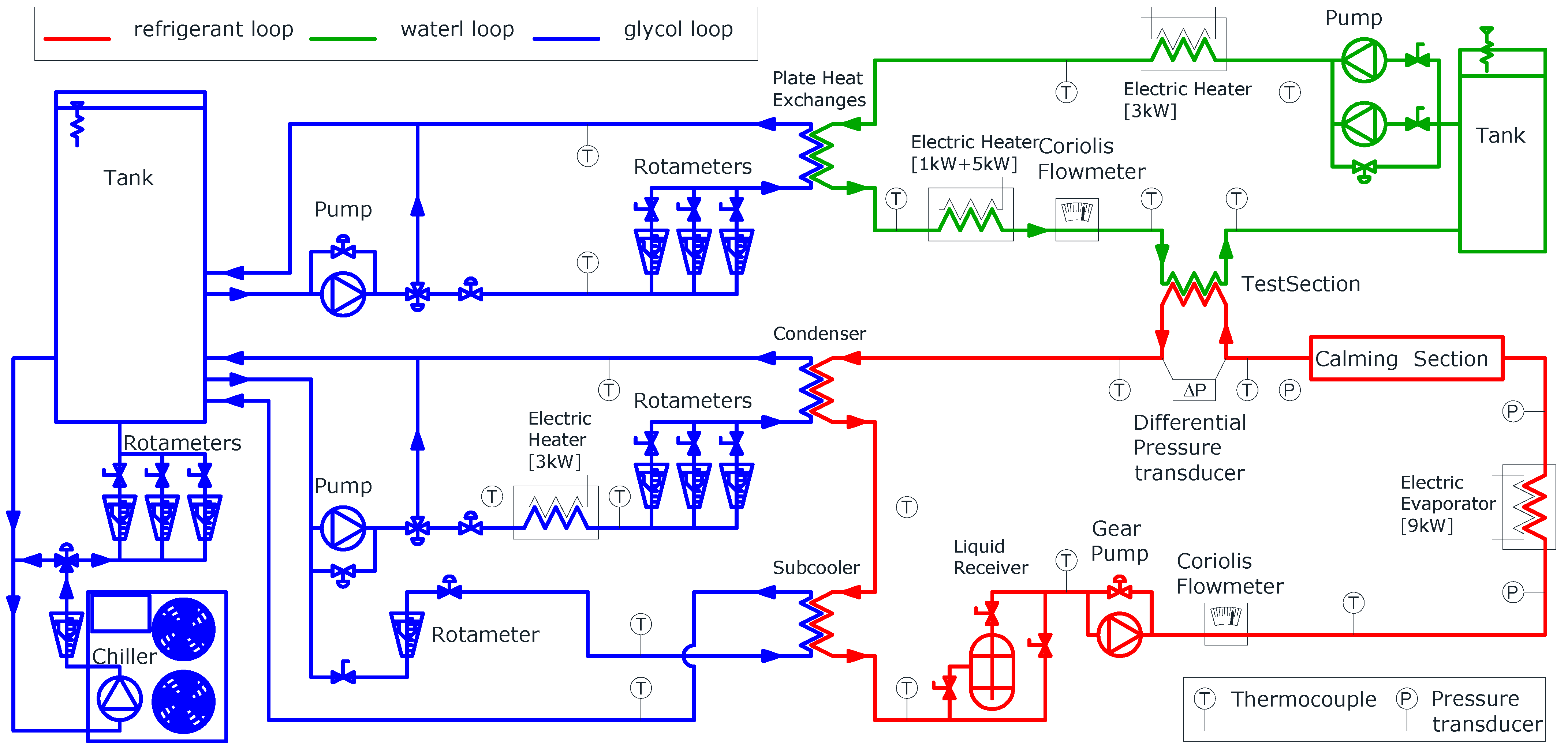
GWP	[-]	1397

). This refrigerant is a potential drop-in replacement for R404A (GWP 3922) and R507A (GWP 3985). The experimental setup, briefly described here (Figure 1) and consisting of three circuits, is explained in greater detail by Colombo et al. [28].

In the refrigerant loop (red line in Figure 1), a shell-and-tube condenser supplies liquid refrigerant to the pump. To avoid cavitation, a plate heat exchanger (sub-cooler) cools down the refrigerant after the condenser. A gear pump with an inverter drive maintains a fixed mass flow rate, measured by a Coriolis flowmeter (range: 0 ÷ 400 kg·h⁻¹, uncertainty: ±0.15% of the reading). The refrigerant’s thermodynamic state is monitored by a K-type thermocouple (uncertainty: ±0.5 K) and a pressure transducer (range: −1 ÷ 30 bar, uncertainty: ±1% of full scale) before it enters an electric evaporator (power: 9 kW). Thermal power adjustments are managed through software to achieve a two-phase flow in specified conditions. The shape of the evaporator heaters is designed to promote phase mixing and ensure thermal equilibrium between liquid and vapor. A straight adiabatic calming section (inner diameter: 8.92 mm, length 4.7 m) follows. It is used to make the flow pattern independent of the flow features at the evaporator outlet. The test section consists of a tube-in-tube counterflow heat exchanger (length: 2.6 m, heat transfer length: 2.22 m) thermally insulated with 100 mm-thick rubber foam. The refrigerant flows in the inner tube (geometry described in

Table 3. Smooth tube geometrical features.

Quantity	Unit of Measurement	Symbol	Value
Inner diameter	[mm]	DI	8.92
Outer Diameter	[mm]	DO	9.52
Wet perimeter	[mm]	P	28.0
Cross-section area	[mm2]	A	62.5
Hydraulic diameter	[mm]	DH	8.92

) while demineralised water passes through the annulus. The refrigerant inlet pressure is measured by an absolute pressure transducer (range: 0 ÷ 16 bar, uncertainty: ±0.25% of full scale). A differential pressure transducer (range: −3.5 ÷ 3.5 bar, uncertainty: ±0.1% of full scale) measures pressure drop. K-type thermocouples (uncertainty: ±0.5 K) measure the inlet and outlet temperatures of the refrigerant. Wall temperature is calculated as the average of three thermocouples placed in grooves (length: 50 mm, depth: 0.15 mm, width: 0.4 mm) machined on the exterior of the inner tube at the inlet and outlet. Thermocouple reference junctions are submerged in Dewar flasks with melting ice to ensure accuracy. The refrigerant leaving the test section returns to the condenser.

The water circuit (green line in Figure 1) exchanges thermal power with the refrigerant to induce phase change. A Coriolis flowmeter (range: 0 ÷ 400 kg·h⁻¹, uncertainty: ±0.15% of reading) measures the water flow rate. Water is supplied from an insulated tank, with flow regulated by bypass or needle valves. Successively, the water is cooled by a water and glycol mixture in a plate heat exchanger, which is followed by a PID-controlled 6 kW electric heater to set the inlet temperatures in the test section. Water inlet and outlet temperatures are recorded using three thermocouples connected in series (K-type, uncertainty: ±0.1 K).

In the glycol loop (blue line in Figure 1), a commercial chiller (cooling capacity: 21 kW) cools a water-glycol mixture (30% glycol by volume; freezing point: −17 °C; operating temperature: −10 °C) stored in a tank. Two circuits, one for water and another for refrigerant, supply the corresponding heat exchangers. The former cools the demineralised water, while the latter manages the test section inlet pressure and prevents cavitation in the refrigerant pump. A manual needle valve regulates the glycol mass flow rate, while a PID-controlled 3 kW electric heater sets the condenser inlet temperature to match refrigerant saturation pressure.

3. Data Sampling

During each test, 181 samples for each quantity were collected at a sampling frequency of 1 Hz, with their mean values serving as the output. To ensure repeatability, the acquisition procedure mandates that each experiment be conducted 10 times, with the mean values of these tests used as the final output. The operating conditions are uniquely defined by three parameters:

• the refrigerant pressure at the test section inlet (p_rTi);
• the refrigerant mass flux (G);
• the bubble temperature (T_b).

4. Data Processing

After an experiment is completed, the instrument readings are processed assuming that

• steady-state operating conditions are met (data is processed only if the variations in quantities remain within ±3% and temperature fluctuations are within ±0.3 K);
• thermal dispersions are negligible (single-phase tests have shown that the difference between refrigerant-side thermal power and waterside thermal power in the test section does not exceed 5%);
• the thermal resistance of the copper tube is negligible (a posteriori calculations indicate it is two orders of magnitude smaller than the refrigerant’s thermal resistance);
• the fouling effect is negligible (the refrigerant circulation pump is a magnetically driven gear-type pump that operates without the need for lubricant).

The post-processing yields three primary outputs:

• the operating conditions (p_rTi, G, T_b, Δx, x_m);
• the total pressure drop per unit length (Z);
• the heat transfer coefficient (h).

Uncertainties for these outputs are calculated using the values in

Table 4. Uncertainties affecting the heat transfer coefficient.

Quantity	Unit of Measurement	Value
Mass flow rate (water/refrigerant)	[-]	±0.15% of the reading
Temperature	[K]	±0.5
Operating pressure	[bar]	±0.025
Pressure drop	[kPa]	±0.35
Evaporator power	[kW]	±0.09

and the uncertainty propagation algorithm described by Moffat [29]. For a quantity y, which depends on n independent variables x_j, the absolute uncertainty (U_y) is determined by

$$U_y=\sqrt{{\sum }_{j=1}^n{\left(U_{x_j}{\displaystyle \frac{\partial y}{\partial x_j}}\right)}^2}$$

(1)

The refrigerant pressure at the test section inlet, p_rti, is measured by an absolute pressure transducer, while the temperature at the same location, T_rti, is recorded using a thermocouple. The bubble temperature T_b is computed using the measured pressure, p_rti, as input for the software RefProp 10.

The mass flux G is calculated as the ratio of the refrigerant mass flow rate, m_r, to the duct’s cross-sectional area, A_c:

$$G={\displaystyle \frac{m_r}{A_c}}$$

(2)

The refrigerant quality change within the test section is determined based on the refrigerant’s pressure and enthalpy at the inlet and outlet. The outlet pressure, p_rto, is derived by subtracting the pressure drop (Δp > 0) measured by the differential pressure transducer from the inlet pressure:

$$p_{rTo}=p_{rTi}-∆p$$

(3)

The test section inlet enthalpy, i_rti, is calculated using the energy balance at the evaporator. The enthalpy of the subcooled liquid at the evaporator inlet, i_rei, is obtained using NIST RefProp 10 based on the evaporator inlet temperature, T_rei, and pressure, p_rei:

$$i_{rEi}=i(T_{rEi},p_{rEi})$$

(4)

The evaporator’s thermal power, Q_E, is measured by a net analyser, and the evaporator outlet enthalpy, which corresponds to the test section inlet enthalpy, is computed as:

$$i_{rTi}=i_{rEi}+{\displaystyle \frac{Q_E}{m_r}}$$

(5)

The test section outlet enthalpy, i_rTo, is determined using the energy balance for the test section:

$$i_{rTo}=i_{rTi}+{\displaystyle \frac{m_a{c}_{pa}\left(T_{aTi}-T_{aTo}\right)}{m_r}}$$

(6)

The refrigerant inlet quality, x_Ti, and outlet quality, x_To, are calculated using RefProp 10 with pressure and enthalpy as inputs at the corresponding positions:

$$x_{Ti}=x\left(p_{rTi},i_{rTi}\right)$$

(7)

$$x_{To}=x\left(p_{rTo},i_{rTo}\right)$$

(8)

The quality change, Δx, and the mean quality, x_m, are determined as follows:

$$∆x=x_{Ti}-x_{To}$$

(9)

$$x_m={\displaystyle \frac{x_{To}+x_{Ti}}{2}}$$

(10)

The total pressure drop, Δp, is measured using a differential pressure transducer. The pressure gradient Z (with an uncertainty below 4%) is obtained as:

$$Z={\displaystyle \frac{∆p}{L}}$$

(11)

The heat transfer coefficient h, relative to the inner tube surface, is determined using the logarithmic mean temperature difference, ΔT_lm, calculated based on the refrigerant and wall temperatures. The wall temperature T_w is the average of the readings from thermocouples glued to the outside of the copper tube:

$$T_w={\displaystyle \frac{T_b+T_s+T_t}{3}}$$

(12)

The logarithmic mean temperature difference is expressed as:

$${∆T}_{lm}={\displaystyle \frac{\left(T_{wo}-T_{rTo}\right)-\left(T_{wi}-T_{rTi}\right)}{\ln \frac{T_{wo}-T_{rTo}}{T_{wi}-T_{rTi}}}}$$

(13)

This temperature difference is then used to compute the heat transfer coefficient:

$$h={\displaystyle \frac{Q_T}{\pi D_{I}l{∆T}_{lm}}}$$

(14)

5. Results

The experiments aim to study the effect of the temperature on the pressure drop per unit length Z and the heat transfer coefficient h during full evaporation inside a horizontal smooth tube. As the R449a is a zeotropic mixture, during phase change, the temperature varies, and the experimental conditions are identified according to the operating pressure p and the corresponding bubble temperature T_b. These two quantities span the ranges p ∈ [662;833] kPa and T_b ∈ [2.5;10] °C, respectively. In

Table 5. R449a thermal properties at the operating pressures: liquid, at bubble temperature T_b, and vapor, at dew temperature T_d.

		Liquid Phase at Bubble Temperature Tb					Vapour Phase at Dew Temperature Td
p	Td-Tb	Tb	ρ	k	μ	σ	Tb	ρ	k	μ	σ
[kPa]	[°C]	[°C]	[kg·m−3]	[W·m−1·K−1]	[Pa·s]	[N·m]	[°C]	[kg·m−3]	[W·m−1·K−1]	[Pa·s]	[N·m]
662	5.2	2.5	1188	9.05·10−2	1.84·10−4	9.04·10−3	7.7	29.0	1.28·10−2	1.17·10−5	8.55·10−3
716	5.1	5.0	1179	8.93·10−2	1.78·10−4	8.68·10−3	10.1	31.3	1.30·10−2	1.18·10−5	8.19·10−3
773	5.1	7.5	1169	8.82·10−2	1.73·10−4	8.31·10−3	12.6	33.8	1.33·10−2	1.19·10−5	7.84·10−3
833	5.1	10.0	1160	8.70·10−2	1.68·10−4	7.95·10−3	15.1	36.5	1.35·10−2	1.20·10−5	7.49·10−3

, the values of the quantities identifying the operating conditions tested during the experiments are reported together with the thermal properties affecting the pressure drop per unit length and the heat transfer coefficient in flow boiling. The properties were evaluated for the liquid phase at the bubble temperature T_b and the vapour phase at the dew temperature T_d. Because the temperature glide takes place during evaporation, the average temperature between the inlet and outlet of the test section was used to compute the thermal properties required for the data processing, whose values are reported in

Table 6. Liquid and vapour R449a thermal properties at the mean operating temperatures T_m.

		Liquid Phase					Vapour Phase
Tm	p	ρ	k	μ	ρ	k	μ	ρlv = ρl/ρv	klv = kl/kv	μlv = μl/μv	Tm
[°C]	[kPa]	[kg·m−3]	[W·m−1·K−1]	[Pa·s]	[kg·m−3]	[W·m−1·K−1]	[Pa·s]	[-]	[-]	[-]	[°C]
5.0	716	1179	8.93·10−2	1.78·10−4	29.2	1.26·10−2	1.18·10−5	40.4	7.1	15.1	5.0
7.5	773	1169	8.82·10−2	1.73·10−4	31.5	1.28·10−2	1.19·10−5	37.1	6.9	14.5	7.5
10.0	833	1160	8.70·10−2	1.68·10−4	34.1	1.31·10−2	1.20·10−5	34.1	6.6	13.9	10.0
12.5	896	1150	8.58·10−2	1.63·10−4	36.8	1.34·10−2	1.21·10−5	31.3	6.4	13.4	12.5

.

Table 7. Effect of the temperature on liquid and vapour R449a thermal properties, percentage variation Δg_% = g(T)/g(T_r) − 1, reference temperature T_r = 5 °C.

		Liquid Phase				Vapour Phase
Tm	Δp%	Δρ%	Δk%	Δμ%	Δρ%	Δk%	Δμ%	Δρlv%	Δklv%	Δμlv%
7.5	8%	−0.8%	−1.3%	−3.0%	8.1%	2.0%	0.9%	−8.3%	−3.2%	−3.9%
10.0	16%	−1.6%	−2.7%	−6.0%	16.8%	4.0%	1.8%	−15.8%	−6.4%	−7.6%
12.5	25%	−2.5%	−4.0%	−8.8%	26.0%	6.2%	2.7%	−22.6%	−9.5%	−11.2%

shows their percentage variation, which is calculated according to Equation (15), with g as a generic quantity and selecting the smallest mean temperature as the reference temperature, T_r = 5 °C:

$${∆g}_{\%}={\displaystyle \frac{g\left(T\right)}{g\left(T_r\right)}}-1$$

(15)

To avoid spurious effects connected with the single-phase flow and, at the same time, perform experiments representative of full evaporation in similar operating conditions, nominal inlet and outlet qualities of x_Ti = 0.1 and x_To = 0.9 were selected, respectively, while the nominal outlet wall temperature was set T_wo = 25 °C to properly analyse the effect of the mass flux. The tests were considered suitable for post-processing if all the following constraints were fulfilled:

• inlet quality in the range: x_Ti ∈ [0.04;0.14];
• outlet quality in the range: x_To ∈ [0.75;0.95];
• quality change in the range: Δx ∈ [0.7;0.9];
• the outlet wall temperature is in the range T_wo ∈ [22.5;27.5] °C.

Figure 2 reports the four flow pattern maps, sorted according to the bubble temperature, which highlights the inlet quality x_Ti (blue triangles pointing to the right), the mean quality x_m (blue dots), and the outlet quality x_To (blue triangles pointing to the left).

It is useful to highlight some remarks to analyse the heat transfer performances.

A.

Compared to the vapour density, the density of the liquid phase, as reported in

Table 8. Pressure drop per unit length: comparison between experimental data and predictions of the correlations.

	E%	EA%	σ%	X30%		E%	EA%	σ%	X30%
Zhang-Webb [23]	1.8%	15.1%	22.4%	88%	Dione-(H) [16]	52.7%	52.7%	46.9%	38%
Sun-Mishima [25]	−0.6%	18.2%	25.9%	88%	Yang et al. [26]	−35.1%	36.4%	15.0%	25%
Shannak [24]	−6.1%	19.3%	24.0%	88%	Kuo-Wang [22]	64.8%	64.8%	39.0%	13%
Sugita et al. [27]	−14.1%	20.7%	19.0%	79%	Dione-(S) [16]	67.7%	67.7%	47.5%	13%
Choi et al. [20]	−16.6%	23.7%	21.4%	71%

, is almost forty to thirty times larger; moreover, as shown in

Table 9. Heat transfer coefficient: comparison between experimental data and predictions of the correlations. (*) use of the Bell and Ghali corrections.

	E%	EA%	σ%	X30%		E%	EA%	σ%	X30%
Bertsch [12]	−11.8%	14.0%	11.2%	100%	Wattelet * [7]	26.2%	26.2%	20.0%	58%
Gungor-Winterton [5]	7.4%	16.5%	19.3%	88%	Liu-Winterton [6]	27.3%	27.3%	19.6%	54%
Dione [16]	−4.6%	18.0%	20.9%	88%	Kew-Cornwell [9]	43.9%	43.9%	30.1%	42%
Kim-Mudawar [14]	9.2%	16.0%	18.5%	83%	Kattan [8]	44.6%	44.6%	21.6%	38%
Del Col * [13]	9.2%	16.8%	19.9%	83%	Boissieu [10]	44.6%	44.6%	21.6%	38%
Wojtan [11]	15.7%	18.4%	17.3%	79%	Del Col [13]	51.1%	51.1%	27.1%	17%
Shah [4]	19.5%	20.1%	20.0%	67%	Wattelet [7]	79.4%	79.4%	26.7%	0%
Wongsa-Ngam [2]	−19.4%	21.1%	14.3%	62%

, the ratio decreases as the mean temperature rises.

B.

The thermal conductivity of the liquid phase slightly decreases (Table 8) as the mean temperature increases, while, for the vapor, the opposite happens. In absolute terms, the variation for the vapour is larger than the one for the liquid; therefore, in the selected temperature range, the ratio between the liquid thermal conductivity and the vapour thermal conductivity monotonically decreases from 7.1 to 6.4.

C.

Because of remark A, during the experiments, vapour occupies the largest part of the cross-sectional area (e.g., in case x = 0.1, the smallest value of the volume fraction is 76%).

D.

In the intermittent flow, the effects of gravity and shear stress are comparable, and the liquid adjoins a significant portion of the cross-sectional perimeter periodically. The heat transfer performances of the flow are influenced by the thermal conductivities of both liquid and vapor.

E.

In the annular flow, the shear stress effect overcomes the gravity effect, and the liquid is arranged all around the cross-sectional perimeter in an almost uniform layer. The heat transfer performances of the flow are mainly related to the liquid thermal conductivity.

F.

In a horizontal smooth tube, the dry-out phenomenon takes place in the quality range x ∈ [0.6;0.7].

G.

As long as the quality change Δx and the mean quality x_m are the same, because of remarks B, D, and E, it could be expected that the heat transfer performance of intermittent flow is worse than the annular flow.

H.

According to Figure 3, which displays the flow regimes onsetting in the test section during the experiments, because of remarks C, D, and F, it seems that the largest part of the test section wall surface is adjoined by the vapour phase.

5.1. Pressure Drop per Unit Length

As highlighted in Figure 2, for all the operating conditions, there is a slug or intermittent flow at the test section inlet, and, as the evaporation takes place and the quality increases, it is replaced by an annular flow. According to the flow pattern maps, the higher the mass flux, the wider is the portion of the test section with annular flow.

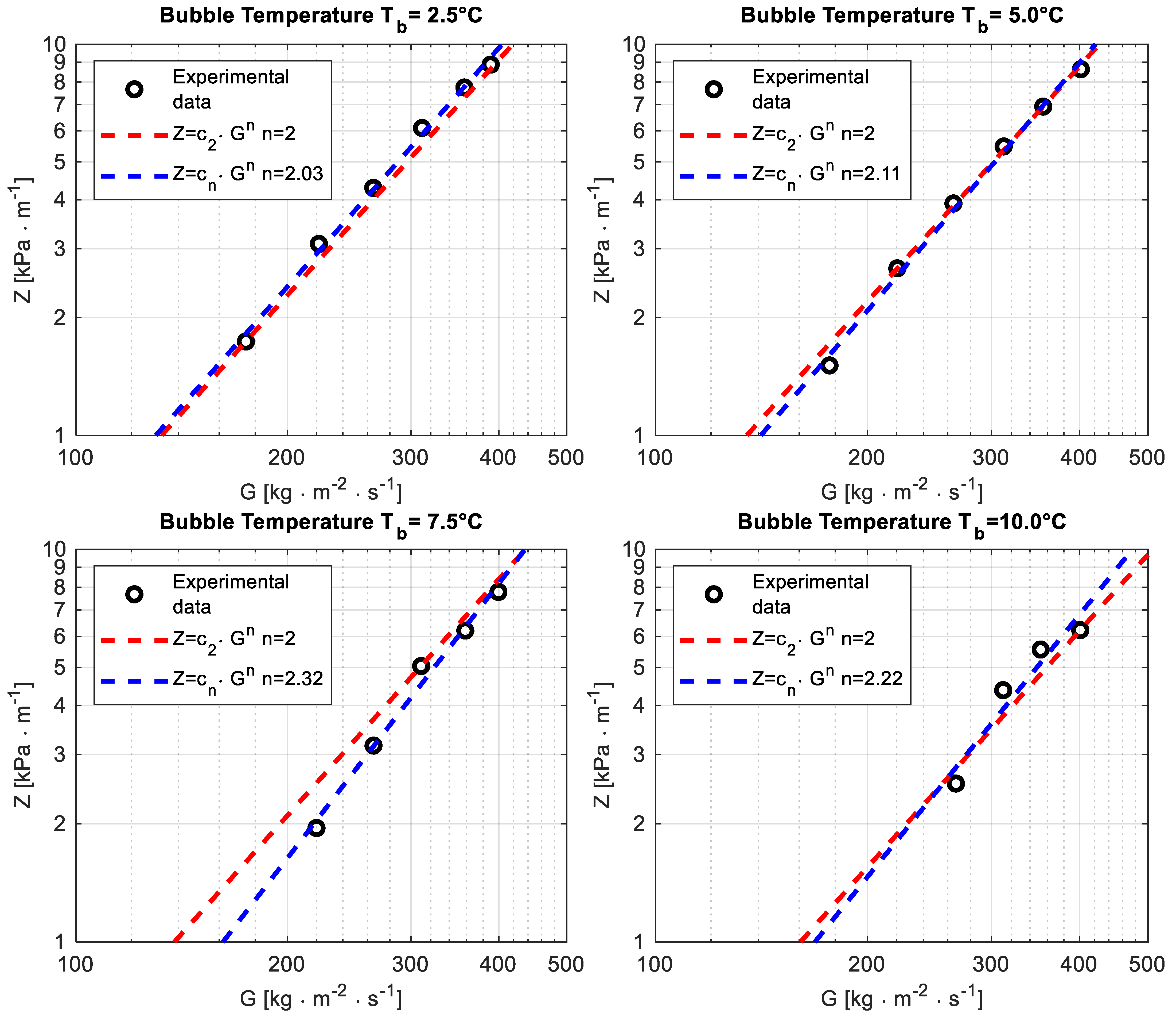
The fitting of pressure drop per unit length as a function of the mass flux using a power law, performed as a preliminary test, highlighted an exponent n close to 2 in the range n ∈ [2.03;2.32], which is consistent with the theory and suggests that the data are reliable. The outcome of the fitting is reported for the four operating bubble temperatures in Figure 3 (because of the limit of the differential pressure transducer, it was not possible to properly read the pressure drop in some operating conditions tested for bubble temperatures T_b = 7.5 °C and T_b = 10 °C).

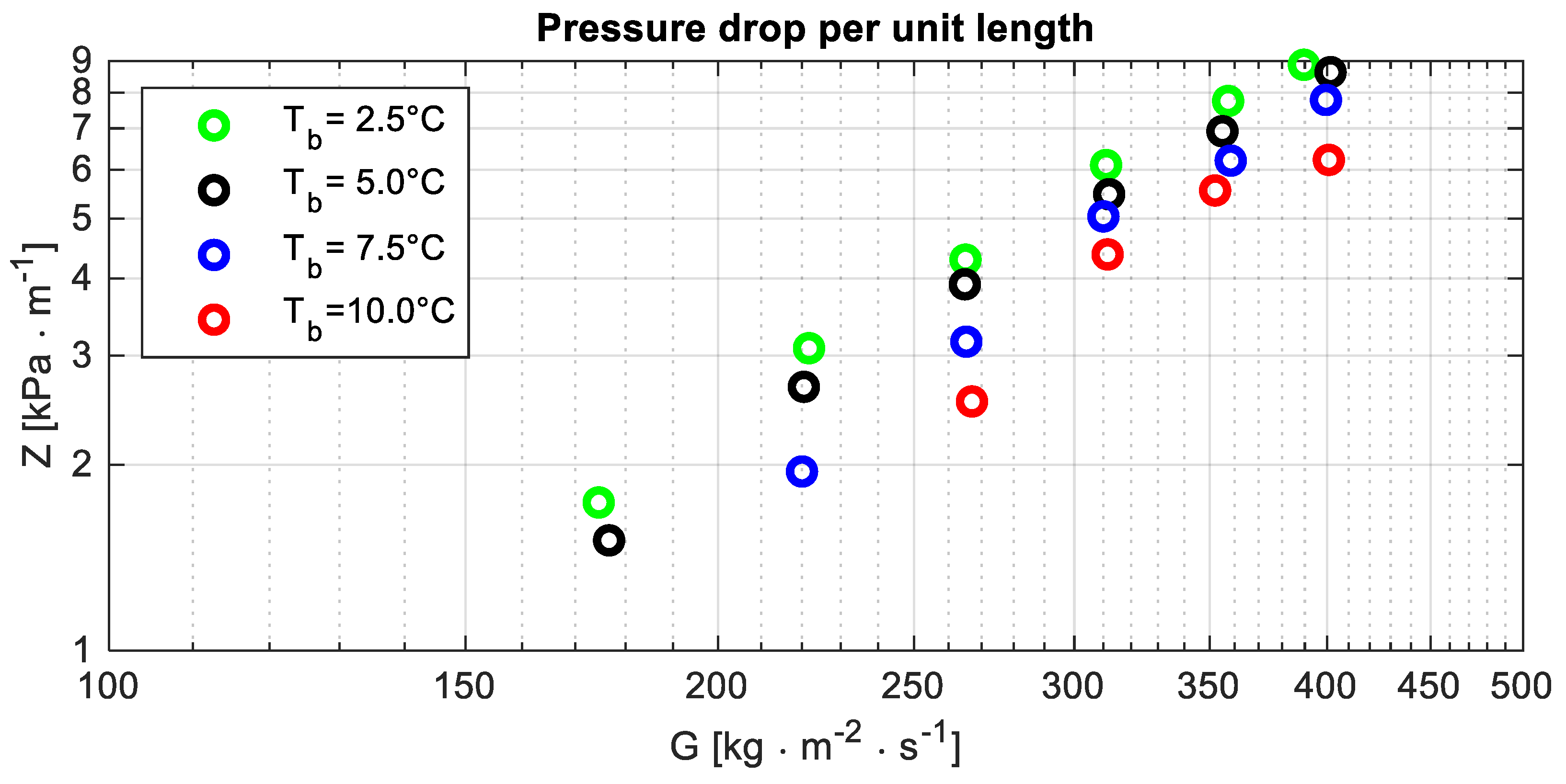
All the data concerning the pressure drop per unit length are displayed in Figure 4, which shows that the pressure drop per unit length reduces as the temperature increases. That could be explained by considering the following notes.

• Because of remark F, the pressure drop per unit length is mainly affected by the vapour dynamic viscosity. According to Table 9, that quantity seems unaffected by the temperature in the range T_m ∈ [5;12.5] °C tested during the experimental activity: Table 9 reports a percentage variation Δμ_% < 3%.
• The dynamic viscosity of the liquid phase reduces as the temperature increases (Table 9): between the smallest and the largest temperature, its percentage variation is almost 10% (Δμ_% = −8.8%).
• Because of remarks D, it could be expected that the velocity gradient in a cross-section is mainly related to the vapour velocity. From remark A, it follows that, for a fixed mass flux, the mean vapour velocity reduces as the temperature increases. The percentage reduction of the mean velocity is approximately of the same order of magnitude, with the opposite sign of the density percentage variation.
• The combined effects of the aforementioned factors account for the reduction of the pressure drop per unit length as the temperature increases.

5.2. Heat Transfer Coefficient

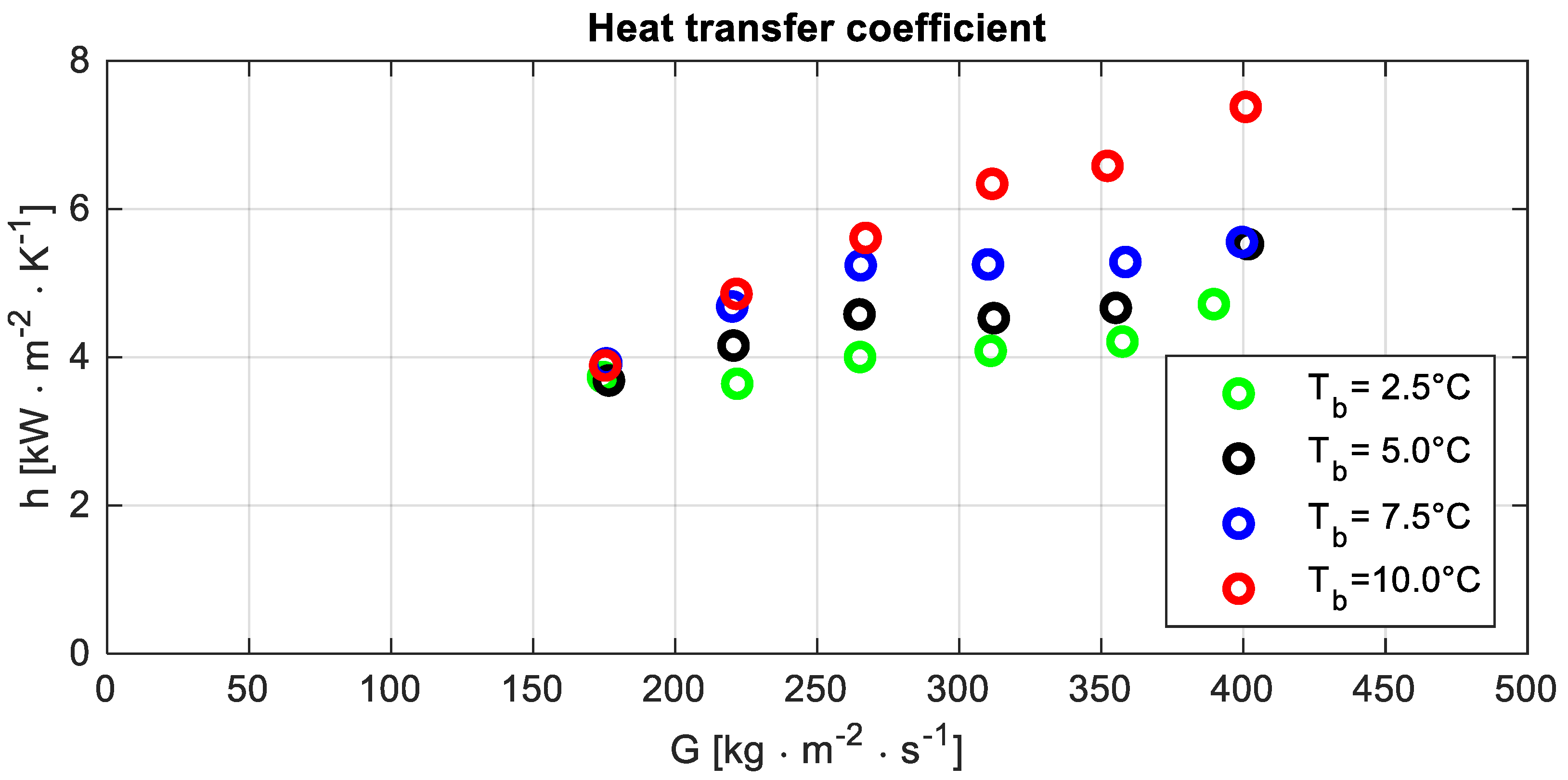
The outcome of the experiments, which is reported in Figure 5, highlighted the increase of the heat transfer coefficient when the operating temperature grows. A possible explanation could be linked to remarks H and B, which, respectively, mention that the test section wall is mainly adjoined by the vapour phase and the thermal conductivity of vapour increases with the operating temperature.

Figure 5 shows a difference in the trend of the heat transfer coefficient as a function of the mass flux at bubble temperature T_b = 10 °C compared to other operating conditions. It could be a consequence of the smaller outlet quality. Because of that, a shorter portion of the test section is characterised by the dry-out condition, and a larger heat transfer coefficient could be expected.

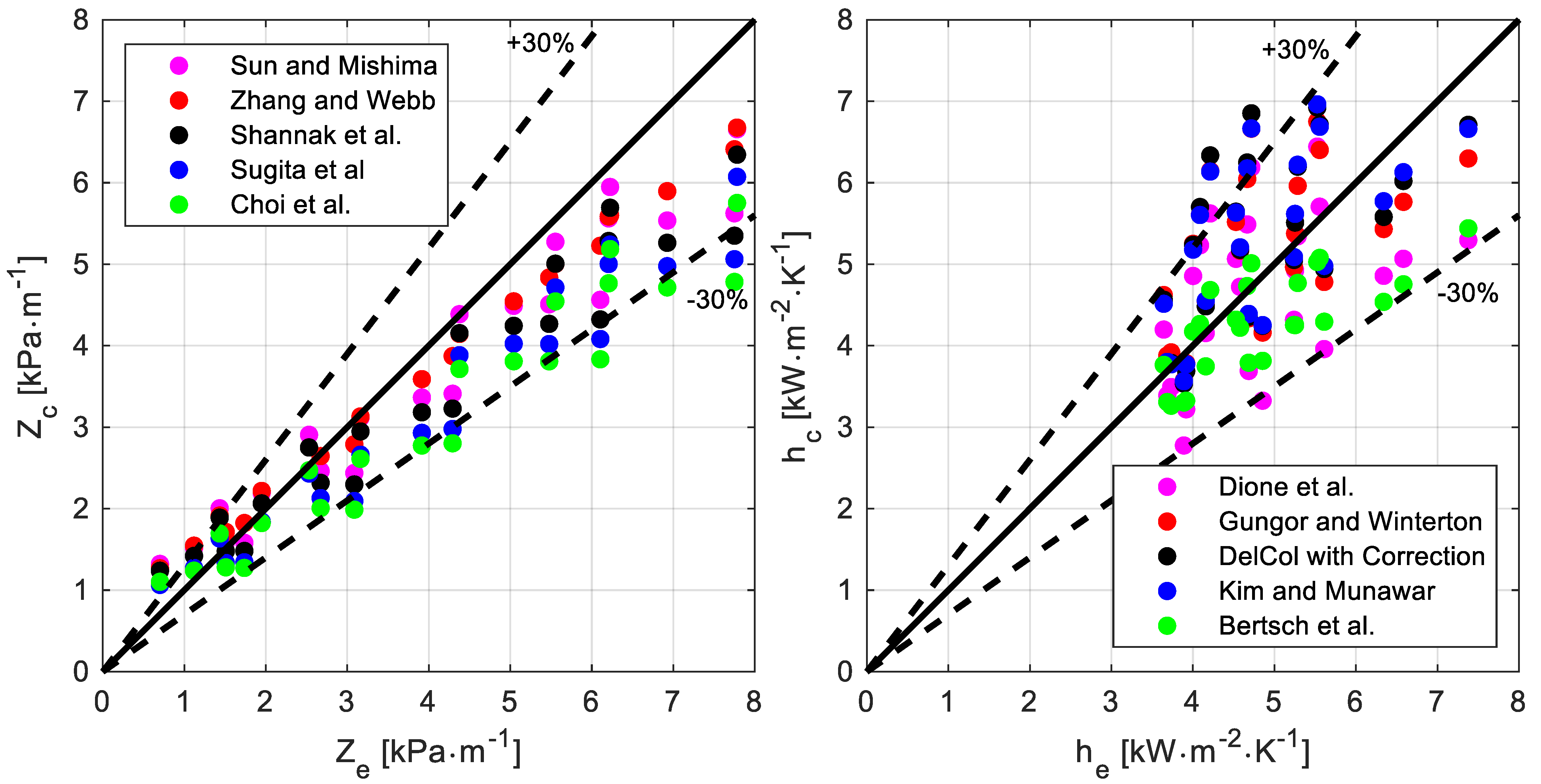
5.3. Comparison Between Data and Correlations

In the end, the experimental results concerning the pressure drop per unit length Z and the heat transfer coefficient h, collected during the tests performed at the different bubble temperatures T_b, were compared with the predictions of the correlations available in the open literature on the basis of the four indexes.

• The mean percentage error E_%:

$$E_{\%}={\displaystyle \frac{1}{N}}\sum _{j=1}^N\left({\displaystyle \frac{g_{cj}}{g_{ej}}}-1\right)$$

(16)

• The mean absolute percentage deviation E_a%:

$$E_{A\%}={\displaystyle \frac{1}{N}}\sum _{j=1}^N\left|{\displaystyle \frac{g_{cj}}{g_{ej}}}-1\right|$$

(17)

• The standard deviation of the mean percentage error σ_%:

$${\sigma }_{\%}=\sqrt{{\displaystyle \frac{1}{N}}\sum _{j=1}^N{\left[\left({\displaystyle \frac{g_{cj}}{g_{ej}}}-1\right)-E_{\%}\right]}^2}$$

(18)

• The percentage of the predictions X₃₀ with ±30% of the experimental data:

$$X_{30}={\displaystyle \frac{N_{30}}{N}}$$

(19)

Nine correlations were selected to predict the pressure drop per unit length Z. All the models, except one, only provide the frictional pressure drop per unit length. Instead, in Choi et al. [20], the focus is the total pressure drop per unit length, which is the quantity that is possible to measure in the experiments. Their model suggests computing the accelerative pressure drop to rely on the Rouhani and Axelsson correlation [18] for the void fraction. In the present analysis, the accelerative pressure per unit length, as specified by Choi et al. [20], was calculated for all the correlations, the total pressure drop per unit length was determined, and the comparison with the experimental data was performed.

The chart on the left in Figure 6 displays the parity plot of the five best-performing (based on the index X₃₀) correlations to predict the pressure drop per unit length. The numerical values listed in Table 8 (sorted for decreasing value of the index X₃₀) show that among all the considered correlations, three of them (namely, Zhang-Webb, Sun-Mishima, and Shannak) are capable of adequately accounting for the temperature effect, and their performances are good and comparable. The X₃₀ is the same for all of them, while the other indexes have only a marginal difference.

Fifteen correlations were compared with the experimental data; they are listed in Table 9, sorted for decreasing value of the index X₃₀, while the chart on the right in Figure 6 displays the parity plot of the best-performing five (according to the X₃₀ values). Even though five correlations proved to properly predict the heat transfer coefficient and account for the temperature effect, the Bertsch correlation performs best (X₃₀ = 100%, E_A% = 14%). It is also interesting to highlight that the Bell and Ghali correction, originally developed to extend results for pure fluids to zeotropic mixtures during convective condensation, also seems to work for evaporation. For instance, the worst-performing correlations (Del Col and Wattelet), which were developed using a database involving pure fluids only, significantly improve their indexes (especially the former) when the Bell and Ghali correction is used to account for the resistance to mass transfer.

6. Conclusions

A set of experiments concerning operating conditions that properly approximate complete evaporation (inlet quality in the range: x_Ti ∈ [0.04;0.14], outlet quality in the range: x_To ∈ [0.75;0.95], quality change in the range: Δx ∈ [0.7;0.9]) was performed at six different mass fluxes in the range G ∈ [175;400] kg·m⁻²·s⁻¹ to test the effect of the temperature, which was identified by the bubble temperature, on the pressure drop per unit length and the heat transfer coefficient. The experimental activity highlighted that the pressure drop per unit length reduces as the bubble temperature increases, while the opposite happens for the heat transfer coefficient. When comparing the data with the predictions of the correlations for the pressure drop per unit length, three of them were found to have similar, best-performing indexes. Finally, regarding the heat transfer coefficient, the Bertsch correlation performed best (X₃₀ = 100%, E_A% = 14%).