Article

Optimizing Computational Process of High-Order Taylor Discontinuous Galerkin Method for Solving the Euler Equations

1
Graduate School of Science and Technology, University of Tsukuba, Tsukuba 305-8573, Japan
2
Institute of Systems and Information Engineering, University of Tsukuba, Tsukuba 305-8573, Japan
*
Author to whom correspondence should be addressed.
Appl. Sci. 2025, 15(7), 4047; https://doi.org/10.3390/app15074047
Submission received: 23 February 2025 / Revised: 22 March 2025 / Accepted: 25 March 2025 / Published: 7 April 2025

Abstract

:
Solving the Euler equations often requires expensive computations of complex, high-order time derivatives. Although Taylor Discontinuous Galerkin (TDG) schemes are renowned for their accuracy and stability, directly evaluating third-order tensor derivatives can significantly reduce computational efficiency, particularly for large-scale, intricate flow problems. To overcome this difficulty, this paper presents an optimized numerical procedure that combines Taylor series time integration with the Discontinuous Galerkin (DG) approach. By replacing cumbersome tensor derivatives with simpler time derivatives of the Jacobian matrix and finite difference method inside the element to calculate the high-order time derivative terms, the proposed method substantially decreases the computational cost while maintaining accuracy and stability. After verifying its fundamental feasibility in one-dimensional tests, the optimized TDG method is applied to a two-dimensional forward-facing step problem. In all numerical tests, the optimized TDG method clearly exhibits a computational efficiency advantage over the conventional TDG method, therefore saving a great amount of time, nearly 70%. This concept can be naturally extended to higher-dimensional scenarios, offering a promising and efficient tool for large-scale computational fluid dynamics simulations.

1. Introduction

The Euler equations, fundamental to computational fluid dynamics, require high-order temporal accuracy to capture intricate flow features in various engineering and scientific applications. Among numerical methods, the Discontinuous Galerkin (DG) method is particularly notable. It extends the principles of the finite element method (FEM) to offer flexibility for complex geometries, efficient parallelization, and the ability to handle discontinuities at element interfaces [1,2]. Initially developed by Reed and Hill [1] for the neutron transport equation, the DG method was subsequently adapted for polynomial-based approximations [2]. Cockburn and colleagues [3,4,5] extended the DG framework to time-dependent problems, integrating the Runge–Kutta (RK) method into the DG framework to establish the RKDG method [6]. This powerful combination refined the approach for conservation laws and ensured convergence, facilitating simulations across diverse fields. In a recent study [7], the phenomenon of the interaction of shock waves with forward-triangular light gas bubbles was simulated using the high-fidelity explicit modal discontinuous Galerkin technique. This work demonstrates that the DG method provides excellent simulation capabilities for complex aerodynamic phenomena by solving the Euler equations. Additionally, this simulation enables in-depth exploration of the impact of different parameter conditions on flow morphology through comparison and observation. The above work demonstrates that using numerical computation methods based on the DG method for simulating fluid problems governed by the Euler equations as the governing equations can obtain excellent results.
The DG method is primarily employed for spatial discretization in time-dependent conservative partial differential equations (PDEs). For temporal discretization, the RK method has become the standard for iteratively calculating temporal derivatives to achieve high-order accuracy. By contrast, the Taylor Discontinuous Galerkin (TDG) method offers an innovative alternative. Instead of relying on multiple low-order predictions typical of RK-based schemes, it directly employs high-order Taylor series expansions derived from the Lax–Wendroff-type time integration scheme [8]. This approach constructs high-order approximations without the need for iterative corrections, which can be computationally expensive, particularly in large-scale (advantage in CPU timing for the same accuracy by TDG) complex systems where the dimensionality and complexity significantly increase computational costs [9].
The potential of Taylor–Galerkin methods was first demonstrated by Donea [10] in solving convective transport problems. Subsequent studies extended their application to incompressible flows involving heat transfer [11] and hyperbolic conservation laws [8]. Its semi-implicit adaptations have further widened its applicability. Qiu [12] highlighted the compactness of the TDG method and its significant time-saving advantages, making it particularly well suited for large-scale simulations. By avoiding the iterative procedures inherent in RK-based schemes, the TDG framework provides a direct and efficient path to achieving high-order temporal accuracy, advancing both computational efficiency and precision in solving Euler equations for large-scale complex phenomena.
Nevertheless, implementing TDG methods for multi-dimensional and large-scale flow problems remains challenging. A key difficulty lies in evaluating the complex third-order tensor derivatives required by standard TDG formulations, which can lead to substantial computational overhead. Although recent modifications that incorporate central difference schemes have helped simplify the computation of high-order temporal derivatives by employing the finite difference method [12], these approaches often demand extensive information from neighboring elements, reducing their efficiency near domain boundaries. Moreover, while one-dimensional tests have successfully validated TDG’s fundamental principles, many practical engineering applications—such as turbulent aeroacoustics, high-speed compressible flows, and multiphase problems—are inherently multi-dimensional and demand more efficient, robust approaches [8,12].
This study addresses these issues by introducing an optimized TDG method that significantly reduces the computational burden of handling high-order derivatives. Instead of directly computing cumbersome third-order tensors, our approach employs temporal derivatives of the Jacobian matrix, thus simplifying the temporal differentiation process and reducing the number of neighboring elements needed for spatial approximations. After confirming the feasibility and accuracy of this optimized approach in one-dimensional settings, we apply it to a two-dimensional forward-facing step problem—a benchmark known for its complexity. The numerical results demonstrate that our optimized TDG method preserves the accuracy and stability expected from TDG techniques while markedly improving computational efficiency. Although the present work focuses on two-dimensional Euler equations, the fundamental concept can be naturally extended to three-dimensional domains, complex boundary conditions, and even coupled multi-physics problems, thereby offering a promising pathway for simulations for large-scale complex systems.
In conventional TDG methods, the high-order construction makes the spatial integration in the DG method extremely complicated and involves the calculation of exact fluxes, which makes it difficult for the efficiency advantage of traditional TDG algorithms to be realized in complex flux problems. In [13], the integral terms were simplified by using high-order difference approximations in each element, which improved computational efficiency while ensuring accuracy. This indicates that using high-order difference methods within elements does not affect the computational accuracy of the TDG method and can enhance computational efficiency. In this study, the approach of using finite high-order difference methods to simplify calculations is considered in Section 3. Other researchers have also focused on simplifying the flux computation and the finite difference form of unknowns. In [14], the TDG method achieved sharper solution profiles near non-smooth areas by locally using finite difference methods to simplify flux computation and adjusting the differential parameters of the unknowns. However, the above improvements do not prevent the emergence of high-order matrix operators (like tensors).
In [15], it was proven that the numerical computation method based on the Taylor expansion of the Lax–Wendroff temporal discretization combined with the DG method can ensure that the computational process of the Euler method maintains the requirement of positivity-preserving under a third-order expansion. This provides a feasible expectation for using the high-order expansion method of TDG to compute the Euler equations.
The implementation details and numerical experiments presented here build upon the methods described in [16]. Following an initial demonstration of how our optimized TDG approach maintains high-order temporal accuracy and simplifies the weak form calculation for flux terms, we will discuss the theoretical formulation in detail, highlight the key modifications introduced, and present comprehensive numerical evidence of the method’s effectiveness. Through these advancements, we aim to refine the TDG framework into a powerful, efficient, and versatile tool for large-scale multi-physics phenomena.

2. Basic Theory

In this section, we establish the common theoretical foundation of the DG and TDG approaches, setting the stage for the optimized approach introduced in this study. While our primary interest lies in two-dimensional Euler equations, this section begins by considering the one-dimensional conservation law system to establish the core concepts. This approach follows a common practice in computational fluid dynamics, where one-dimensional analyses help verify fundamental properties before extending to higher dimensions.

2.1. Common Approach of TDG Methods

Consider a one-dimensional conservation law, defined on a domain Ω, with solution u ( x , t ) and flux f ( u ) :
u t + f x = 0 .
Nodal discontinuous Galerkin (nodal DG) schemes typically approximate the solution u x , t by using its nodal values through a discretization process. However, DG methods offer a more flexible alternative, enabling the approximation of the solution u x , t without discretization strictly based on nodal values. Specifically, in the K-th element, where x lies in the interval x x ( k 1 ) , x ( k ) , the j -th component of the solution u j x , t can be approximated by a dot product of the expansion coefficient vector u j k t and a basis function vector φ x . In this study, the basis functions φ x are chosen as Legendre polynomials [16], which provide orthogonality and optimal convergence properties for polynomial-based approximations. Given that the basis function vector φ has N components, the approximation achieves a polynomial order of ( N 1 ) . Thus, the approximate solution u ¯ t within the K-th element is expressed as:
u ¯ x , t = u ¯ j x , t = i = 1 N u j i k t φ i k x = u j ( k ) φ = Φ T U ,
where Φ is the basis function matrix:
Φ =   O   φ   O   = φ .
The numerical solution and basis functions may have different numbers of components for each element and should therefore be distinguished element-wise. However, for better readability of the equations, the superscript k is omitted. Specifically, the j -th component of the u ¯ vector, u ¯ j , should be expressed as u ¯ j k x , t = u j ( k ) φ k for K-th element (interval x k 1 x k ). For simplicity, it is instead represented as u ¯ j x , t = u j ( k ) φ .
To ensure that the approximation u ¯ ( x , t ) satisfies the governing equation in a weak form, DG methods impose the following integral condition in each element [1]:
x k 1 x k Φ u ¯ t + f x d x = 0 ,
Within this framework, introducing Taylor series expansions for the temporal derivative u ¯ / t enables the construction of TDG methods. By applying high-order Taylor expansions in time, TDG schemes can achieve superior temporal accuracy compared to standard time-stepping methods. This section focuses on a conventional third-order TDG approach [12], which relies on Lax–Wendroff-type time integration to represent the inertia term u ¯ / t at t = t n , in K-th element as:
u ¯ t n = u ¯ t t = t n = u ¯ n + 1 u ¯ n Δ t Δ t 2 2 u ¯ t 2 t = t n Δ t 2 6 3 u ¯ t 3 t = t n             = u ¯ n + 1 u ¯ n Δ t Δ t 2 u ¯ t t n Δ t 2 6 u ¯ t t t n ,
Therefore, the weak formulation of the Euler equations is:
x k 1 x k Φ U n + 1 d x = x k 1 x k Φ U n d x Δ t Φ f n x k 1 x k + Δ t x k 1 x k Φ x f n d x + Δ t 2 2 x k 1 x k Φ u ¯ t t n d x + Δ t 3 6 x k 1 x k Φ u ¯ t t t n d x .
To handle the high-order temporal derivatives, 2 u / t 2 and 3 u / t 3 , appearing in Equation (5), the flux Jacobian matrix A u is defined as:
f u = A u ,
We can use:
f t = f u u t = A u t = A f x .
From Equation (8), the time-derivative terms u ¯ t t n and u ¯ t t t n can be transformed into spatial derivatives by A u and its associated operators. The benefit of this approach is that all the temporal derivative terms in Equation (6) are converted into spatial derivatives, making it possible to obtain a higher-order estimate of the solution by one-step spatial integration. However, it can also be observed that increasing the order of the time Taylor expansion (using the Lax–Wendroff-type formulation) makes the operators related to A u more complex and consequently increases the number of numerical flux computations. To address this issue, the following sections will demonstrate a detailed explanation of how the optimized TDG method differs from the conventional TDG method, along with an outline of its computational procedure.

2.1.1. Differences Between the Conventional TDG and the Optimized TDG

In conventional TDG method, with Equations (7) and (8), the high-order temporal derivatives can be expressed as [12]:
2 u t 2 = t u t = t f x = x f t = x A u t = x A f x ,
Similarly, for the third temporal derivative:
3 u t 3 = t 2 u t 2 = t x A f x = x A t f x + A t f x ,                       = x u t A u f x + A x f t = x A u f x 2 + A x A f x .
At the time = n, the estimated value of the second temporal derivatives can be defined as:
u ¯ t t n = x A f x t = n ,
Similarly, for the third temporal derivative:
u ¯ t t t n = x A u f x 2 + A x A f x t = n .
Then, Equations (11) and (12) are substituted into Equation (6), and the spatial integration to obtain the solution at the next time is performed. This conventional TDG procedure elegantly combines spatial discretization (via DG) and temporal discretization (via Taylor expansions) to achieve high-order accuracy. However, a major limitation arises from the complexity of computing A / u . Even for relatively simple conservation laws, such as the Euler equations, A / u forms a third-order tensor that significantly increases computational overhead and complexity.
To avoid the usage of A / u , in this work, the high-order temporal derivatives are expressed as:
2 u t 2 = t u t = t f x = x A u t ,
3 u t 3 = t 2 u t 2 = t x A u t = x A 2 u t 2 + A t u t ,
According to Equations (13) and (14), at the time = n, the estimated value of the high-order temporal derivatives can be defined as:
u ¯ t t n = x A u t t = n ,
u ¯ t t t n = x A 2 u t 2 + A t u t t = n .
In this work, these new formulations with Equations (15) and (16) utilize A t = A / t instead of A u = A / u , effectively avoiding the computational cost associated with high-order tensor operations while maintaining high temporal accuracy. Figure 1 illustrates difference between A n , A t n , and tensor A u n at time n. This figure highlights how the proposed method simplifies tensor operations, reducing computational overhead.
Obviously, to complete the calculations for Equations (15) and (16), we first need to determine the values of u / t and A / t . Based on Equation (4), the value of u / t can be obtained as follows:
u t = x ( k 1 ) x ( k ) Φ x f ¯ n d x Φ f ¯ x n x k 1 x k .
Since the two-dimensional matrix A t can be expressed in terms of u and u / t , the next equation is written as follows:
A t = A t u ,   u / t .
From this discussion, it is evident that the computational procedure for the optimized TDG method proposed in this work differs from that of the conventional TDG method, which typically begins with a Lax–Wendroff-type time integration scheme and concludes with spatial integration (via the weak formulation of the DG method). In contrast, the optimized TDG method first employs the DG method to perform spatial integration and thus obtain u / t and A t . It then substitutes the time derivative terms into the time Taylor expansion as:
u ¯ n + 1 = u ¯ n + Δ t u ¯ t n + Δ t 2 2 u ¯ t t n + Δ t 3 6 u ¯ t t t n .

2.1.2. The Calculation of High-Order Temporal Derivatives by the Finite Difference Method Outside the Element

Although the computational cost of the optimized TDG method is lower than that of the conventional TDG method, the computational complexity of the high-order temporal derivatives’ estimation process remains significant. In Equations (33) and (34), the computation of spatial differentiation is necessary to estimate high-order temporal derivative terms U t t n and U t t t n . To this end, this study uses the computational strategy optimized in [
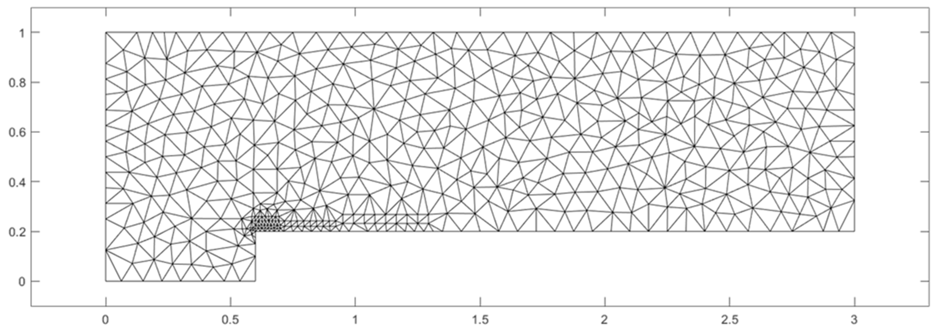
8], which applies the FDM to simplify the spatial differentiation calculation procedure. Although the nodal DG method is employed for spatial discretization in this study, the FDM is applied to the discrete nodes. The discrete nodes and elements constructed by the nodal DG method are illustrated in Figure 2.
When the nodal DG method is used, an estimated solution u ( k , i ) n and an inertia term for a discrete point i in an element K at a time n can be obtained directly by calculating the spatial integral. Consequently, the value of matrix A ( k , i ) n at a point i can be obtained.
According to Equations (15) and (16), functions G ( k , i ) n and H ( k , i ) n are derived as follows:
G ( k , i ) n = A ( k , i ) n u ( k , i ) n ( x ) t t = n ,
H ( k , i ) n = A ( k , i ) n 2 u ( k , i ) n ( x ) t 2 + A ( k , i ) n t u ( k , i ) n ( x ) t t = n .
where n , k , and i denote the time, element number, and position number of a point in an element, respectively.
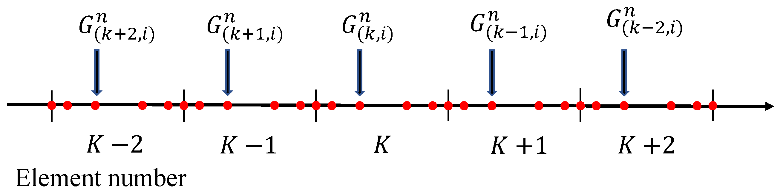
In this study, the fourth-order central difference approximation is used to calculate the high-order temporal derivatives by outside element information. As illustrated in Figure 3, to calculate the high-order temporal derivatives at a target point i in an element K, the values of functions G and H at point i in four elements surrounding the target point must be obtained.
The difference form of the second-order temporal derivative term is calculated by:
2 u k , i n t 2 = 1 12 Δ x G k 2 , i n 8 G k 1 , i n + 8 G k + 1 , i n G k + 2 , i n ,
In the same scheme, the different form of the third-order temporal derivative term is obtained by:
3 u k , i n t 3 = 1 12 Δ x H k 2 , i n 8 H k 1 , i n + 8 H k + 1 , i n H k + 2 , i n .
These operations are used when the optimized method is applied to the test cases presented in this study, which is called the optimized TDG outside element method.

2.1.3. The Calculation of High-Order Temporal Derivatives by the Finite Difference Method Inside the Element

There will be a distinct disadvantage in the above approach, which is that at the boundaries, it is not possible to construct the center difference format directly. At the edges of the computational domain, it is necessary to use one-side difference form. This problem is relatively easy to solve in one-dimensional problems, but for two-dimensional problems it requires a lot of effort to construct the difference form at the boundary. Especially in terms of computational accuracy, to maintain the computational accuracy of the center difference, then at the boundary, it is necessary to construct a difference form that covers the information of multiple cells.
In the optimized TDG method, the nodal DG approach is utilized to discretize elements into a set of discrete points. Based on this discretization, the information at these points can be leveraged to construct new differential forms. These differential forms are primarily required for estimating first-order spatial derivatives. Compared to the modal DG method, the nodal DG approach provides more detailed information within each element, eliminating the need to rely on data from neighboring elements.
If the central difference method is used, the difference formulation within an element is influenced by the positions of the discrete points. This necessitates special handling for the discrete points located at the edges of the element. To address this, the present study employs a higher-order Taylor expansion to construct a differential structure that effectively utilizes the available information at these points. This approach ensures an organized computational framework, where the coefficients of the differential formulation can be precomputed based on the positions of the discrete points. This precomputation is performed while the mesh remains constant, prior to starting the time iteration process.
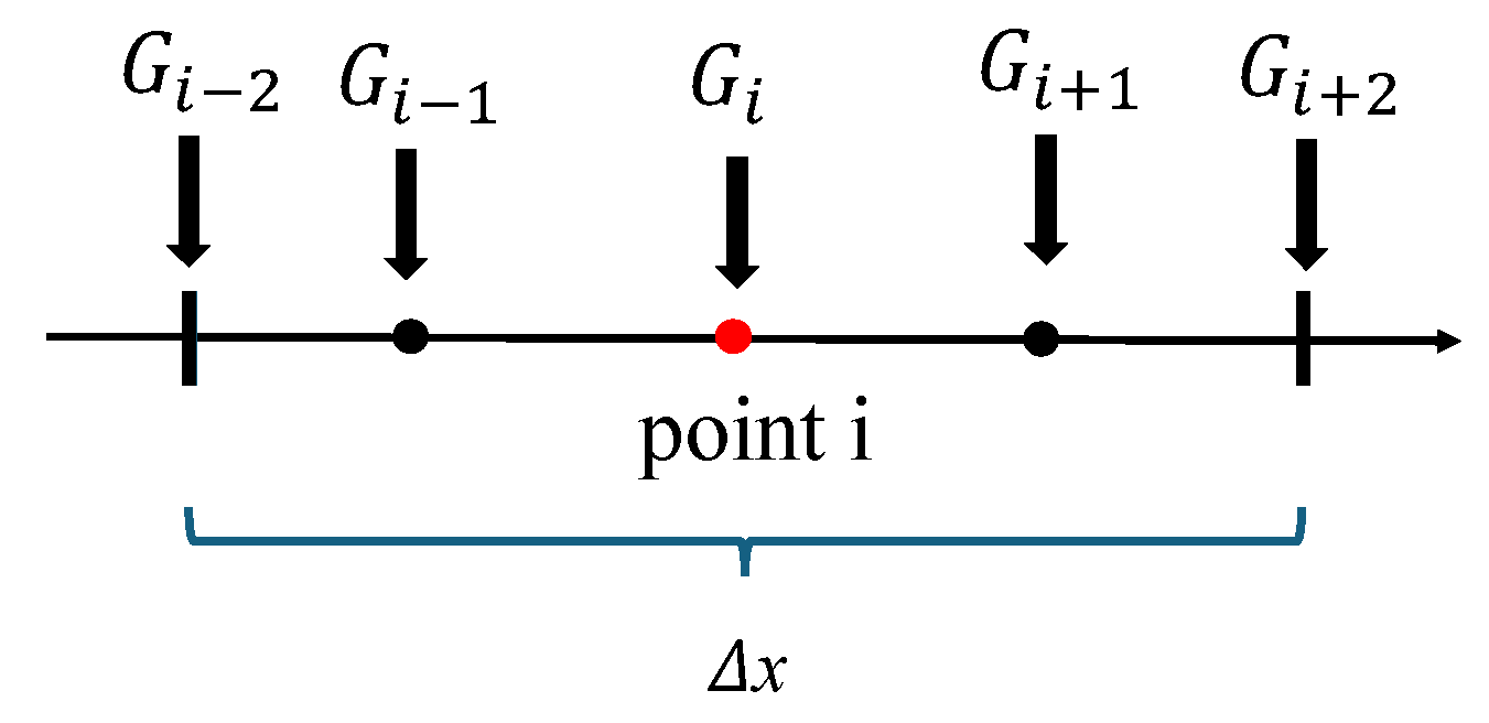
This Taylor difference method estimates the first-order spatial derivatives of unknowns at discrete points by employing the estimated values of all discrete points in one element, as in Figure 3. The process in the one-dimensional format is as follows:
  • Discretization: A one-dimensional segment is treated as a computational element, which is discretized into N points. The estimated values of the governing equations at these points are known;
  • Taylor expansion: For each point x i in the element, the function values at all other points x j j = 1,2 , , , N are expressed using a Taylor series expansion around x i :
    f x j = f x i + x j x i f x i + x j x i 2 2 f x i + + x j x i N N ! f N x i ,
    where f ( x i ) and higher-order derivatives are unknown;
  • Equation system: Using the known function values f x i at the discrete points, the Taylor expansions for all N points are combined to form a system of N equations;
  • Solution: By solving this system of equations, the first-order spatial derivative f ( x i ) is computed for each point x i . Higher-order derivatives may also be obtained if needed, but only the first-order derivative is typically retained in this algorithm;
  • Output: The algorithm produces the first-order spatial derivative f ( x i ) for each point x i in the element and the coefficients a i j ( x i ) of the N equations system. The finite difference function T D x i is:
    f x i = T D x i = j = 1 N a i j ( x i ) f x j .
The above computations correspond to the process of determining finite difference coefficients based on the positions of discrete points. Consequently, this process can be completed before initiating any temporal iterations, and in each subsequent time step, one may directly use the precomputed coefficient matrices. Next, we will illustrate how to compute higher-order temporal derivatives within a one-dimensional element containing five discrete points, once the finite difference coefficients have been obtained using the approach.
According to Equations (15) and (16), functions G ( i ) n and H ( i ) n in k-th element are derived as follows:
G ( i ) n = A ( i ) n u ( i ) n ( x ) t t = n ,
H ( i ) n = A ( i ) n 2 u ( i ) n ( x ) t 2 + A ( i ) n t u ( i ) n ( x ) t t = n ,
where n, k, and i denote the time, element number, and position number of a point in an element, respectively.
As described in Section 2.1.2, in element K, at the time n, with the functions G ( i ) n (24) and H ( i ) n (25), when the N order of polynomials is 4, the difference form of the second-order temporal derivative term is calculated by:
2 u i n t 2 = a i , j 2 G j 2 n + a i , j 1 G j 1 n + a i , j G i , j n + a i , j + 1 G j + 1 n + a i , j + 2 G j + 2 n ,
Since the same finite difference method is employed to compute the first-order spatial derivatives, the coefficients can likewise be used to calculate the third-order temporal-derivative terms by:
3 u i n t 3 = a i , j 2 H j 2 n + a i , j 1 H j 1 n + a i , j H j n + a i , j + 1 H j + 1 n + a i , j + 2 H j + 2 n .
The coefficients vector a and the functions G n , H n vectors in K-th element can be defined as:
a = a i , i 2 , a i , i 1 , a i , a i + 1 , a i + 2 ,
G n = G i 2 n , G i 1 n , G i n , G i + 1 n , G i + 2 n T ,
H n = H i 2 n , H i 1 n , H i n , H i + 1 n , H i + 2 n T .
Since Equations (28)–(30) can be substituted into Equations (26) and (27), the high-order temporal derivatives terms can be calculated as:
2 u i n t 2 = a G n , 3 u i n t 3 = a H n .
Based on the foregoing discussion, the optimized TDG method can be characterized as a hybrid method. Specifically, the first-order temporal derivative at each discrete point is estimated by the DG method from the weak formulation. Subsequently, higher-order temporal derivatives 2 u / t 2 , 3 u / t 3 —commonly employed in the conventional TDG (Lax–Wendroff temporal discretization) framework—are determined by following the approaches outlined in Equations (11) and (12). In this step, the estimated first-order temporal derivative, along with the temporal derivative of matrix A and its higher-order temporal-derivative A / t , are leveraged to infer the 2 u / t 2 and 3 u / t 3 . Thereafter, employing the Taylor series expansion in time allows one to estimate the solution at the next time. Notably, because the higher-order temporal derivatives of matrix A like 2 A / t 2 can be systematically obtained, while maintaining the matrix operators in the two-dimensional matrix form, the usage of the A / U is rendered unnecessary. Therefore, this approach can accommodate higher-order Taylor expansions in time, such as fourth-order or fifth-order expansions, while keeping the temporal derivatives of matrix A in a two-dimensional matrix form, thus avoiding the need for three-dimensional (tensor) or higher-dimensional matrices.

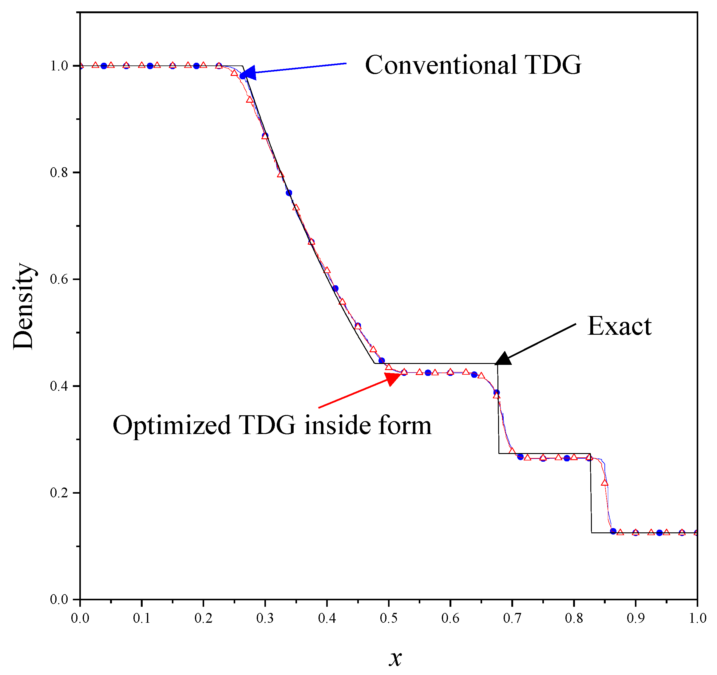
2.2. The Comparison of the Conventional TDG and Optimized TDG

In this section, a comparison is made between the conventional TDG and the optimized TDG (outside form and inside form) by expressing their solutions in an explicit form.
For the conventional TDG method, substituting Equations (11) and (12) into Equation (6), the solutions can be expressed as:
u ¯ n + 1 = u ¯ n + Δ t x ( k 1 ) x ( k ) Φ x f n d x Φ f x n x ( k 1 ) x ( k ) d x   + 1 2 Δ t 2 Φ A n f x n x ( k 1 ) x ( k ) + x ( k 1 ) x ( k ) Φ x A n f x n d x   + 1 6 Δ t 3 Φ A n x A n k f x n x + A n u ¯ f x n 2 | x ( k 1 ) x ( k )   + 1 6 Δ t 3 x ( k 1 ) x ( k ) Φ x A n x A f x n + A u f x n 2 d x .
The above results clearly represent a complete integral form, obtained through spatial integration using the weak formulation. To achieve high-accuracy solutions, ∂A⁄∂U and repeated flux calculations were employed.
For optimized TDG with outside finite difference method, substituting Equations (17), (22), and (23) into Equation (19), the solutions can be expressed as:
u ¯ k , i n + 1 = u ¯ k , i n + Δ t x ( k 1 ) x ( k ) Φ x f ¯ k , i n d x Φ f ¯ k , i n x x k 1 x k d x   Δ t 2 2 1 12 Δ x G k 2 , i n 8 G k 1 , i n + 8 G k + 1 , i n G k + 2 , i n   Δ t 3 6 1 12 Δ x H k 2 , i n 8 H k 1 , i n + 8 H k + 1 , i n H k + 2 , i n .
For optimized TDG with the inside finite difference method, substituting Equations (17) and (31) into Equation (19), the solutions can be expressed as:
u ¯ i n + 1 = u ¯ i n + Δ t x k 1 x k Φ x f ¯ i n d x Φ f ¯ i n x x k 1 x k + Δ t 2 2 a G n + Δ t 3 6 a H n .
Compared to Equation (32), Equations (33) and (34) do not utilize A / U but instead employ the simpler operator A / t , as explained in Section 2.1.2. Furthermore, from Equation (33), it can be observed that the optimized TDG method is a hybrid method combining the DG method and the FDM method. During the application of the FDM method, Equation (33) uses information from elements surrounding the target element for the finite difference calculations. In contrast, Equation (34) demonstrates a way of performing differential calculations using information inside the target element. Clearly, the approach of estimating high-order time derivative terms using internal element information provides better compactness.

3. Results

In this section, both the conventional TDG method and the optimized TDG method are employed to solve the one-dimensional Euler equations in the Sod shock tube problem. The experiment aims to compare the performance of the optimized algorithm using internal interpolation and external finite difference methods. By identifying the approach that delivers higher computational accuracy, the more effective method will then be applied to two-dimensional problems. Finally, a comparative analysis will be conducted on the computational time required to solve two-dimensional Euler problems using the traditional and optimized TDG methods. To ensure consistency in spatial integration across all test cases, this study adopts the nodal DG method with Lagrange polynomials. Additionally, spatial discretization within each element is performed using Legendre–Gauss–Lobatto nodes, as detailed in [16].

3.1. In the One-Dimensional Case

In this section, a one-dimensional shock tube problem is used to demonstrate the performance of the optimized TDG method with third-order Taylor time expansion. It should be noted that the Sod shock tube problem represents a common test case for nonlinear multi-physics problems. The main equations defining the Sod shock problem are the Euler equations, which are expressed as follows:
U t + f x = 0 .
where U is the solution vector, and f is the flux vector. The pressure p can be defined using the two above vectors as follows:
U = ρ , ρ u , e T ;   f = ρ u , ρ u 2 + p , e u + p u T ;   p = γ 1 e u 2 2 ρ .
where ρ represents density, u is velocity, and e denotes energy; γ is the heat capacity ratio, and in this study, it was set to 1.4. In this case, the final time is 0.2 s.
According to the definitions of U and f , a Jacobian Matrix A can be expressed by:
f U = A = 0 1 0 1 2 γ 3 u 2 γ 3 u γ 1 γ 1 u 3 γ e ρ u γ e ρ 3 2 γ 1 u 2 γ u ,
Then, the temporal derivative of Jacobian Matrix ∂A⁄∂t can be calculated as follows:
0 0 0 γ 3 u u t γ 3 u t 0 γ 1 3 u 2 u t γ e t ρ e ρ 2 ρ t u γ e ρ u t γ e t ρ e ρ 2 ρ t 3 γ 1 u u t γ u t .
Table 1 presents a numerical result comparison of the conventional TDG method and the optimized TDG method (outside form and inside form), focusing on the L1 (mean absolute error) and L-infinite (max absolute error) errors, with third-order expansion Taylor time expansion form. The errors were calculated for different element numbers when the basis polynomials were extended to the third order. The errors suggested that the three numerical methods with the limiter had comparable accuracy. The limiter used in the three methods was a nonlinear limiter [16], which could suppress numerical oscillations well. In Table 1, it can be observed that the conventional TDG method and the optimized TDG method (outside form and inside form) maintain similar numerical computational accuracy.
As shown in Table 2, for the computation of the one-dimensional Euler equations, the computational efficiency of optimized TDG is significantly superior to that of conventional TDG when using the third-order Taylor time expansion form. On average, using optimized TDG to calculate the one-dimensional Euler equations can save 90% of the time consumed. The results of density for one-dimensional Euler equations in the Sod shock tube problem are presented in Figure 4. In this work, the numerical experiments employ the same computer system, which is configured with an IntelR i7-9750H CPU, with 32 GB of memory, and Windows 11, with a 64-bit operating system.

3.2. In the Two-Dimensional Case

In this section, a two-dimensional forward-facing step case is used to demonstrate the performance of the optimized TDG method. According to the demonstration of time consuming in Section 3.1, the optimized TDG inside form method obtains better efficiency than the outside form. In two-dimensional test case, the optimized TDG inside form is employed. The main equations defining the shock problem are the Euler equations, which are expressed as follows:
U t + F x + G y = 0 .
where U is the solution vector, and F , G are the flux vectors. The pressure p can be defined using the two above vectors as follows:
U = ρ , u , v , e T ,
F = U u + p 0,1 , 0 , u T ; G = U v + p 0,0 , 1 , v T ,
p = γ 1 e u 2 + v 2 2 ρ .
where ρ represents density, u is velocity, and e denotes energy; γ is the heat capacity ratio, and in this study, it was set to 1.4.
According to the definitions of U and f , a Jacobian Matrix A and B can be expressed by:
F U = A ; A = 0 1 0 0 γ 1 u 2 + v 2 2 u 2 3 γ u 1 γ v γ 1 u v γ 1 2 u 2 + v 2 u H u v H + 1 γ u 2 u 1 γ u v 0 γ u ,
G U = B ; B = 0 0 1 0 u v v u 0 γ 1 u 2 + v 2 2 v 2 γ 1 2 u 2 + v 2 v H v 1 γ v 1 γ u v 3 γ v H + 1 γ v 2 γ 1 γ v .
Here H = e + p / ρ , and the temporal derivative of H is:
d H d t = d e d t + d p d t ρ d ρ d t p ρ 2 .
Then, the temporal derivative of Jacobian Matrix A / t and B / t can be calculated as:
A t = 0 0 0                                                         0 γ 1 u d u d t + v d v d t 2 u d u d t 3 γ d u d t 1 γ d v d t                           0 d u d t v + u d v d t γ 1 2 2 u d u d t + v d v d t u + u 2 + v 2 d u d t d H d t u H d u d t d v d t d H d t + 2 1 γ d v d t d u d t 1 γ d u d t v + u d v d t 0 γ d u d t ,
B t = 0 0 0                                       0 d u d t v + u d v d t d v d t d u d t                                   0 γ 1 u d u d t + v d v d t 2 v d v d t γ 1 2 2 u d u d t + v d v d t v + u 2 + v 2 d v d t d H d t v H d v d t 1 γ d v d t 1 γ d u d t v + u d v d t 3 γ d v d t d H d t + 2 1 γ d v d t 0 γ d v d t .
The computational domain is illustrated in Figure 5. The inflow boundary condition is defined as a uniform Mach 3 flow, while no specific boundary conditions are applied at the outflow. And the mesh of this case is shown in Figure 6. In this computation, the polynomial order is 3, and the final simulation time is 2 s.
Figure 7 demonstrates the results of solving the two-dimensional Euler equations using the conventional TDG method, while Figure 8 presents the results obtained with the optimized TDG method. From the above computational results, the optimized TDG (inside form) method achieves convergence results similar to those of the conventional TDG method. However, as shown in the computational time comparison in Table 3, the optimized TDG method demonstrates a significant efficiency advantage over the conventional TDG method.

4. Conclusions

This paper describes an optimized TDG method designed to address the computational complexity encountered in conventional TDG methods when solving equations with complex flux functions. The optimized algorithm incorporates the Jacobian matrix from the traditional TDG approach, as well as the method for converting temporal derivatives into spatial derivatives. However, it introduces a key improvement, the use of the temporal derivative of the Jacobian matrix A / t , to eliminate the tension matrix A / U that arises in the traditional TDG method. This enhancement not only improves computational efficiency but also maintains the same level of accuracy as the original method. To further simplify the computation method, the optimized TDG method employs the finite difference method to calculate high-order temporal derivative terms. Therefore, it can be said that the optimized TDG method is a hybrid algorithm that combines the DG method and the FDM method.
In this study, two finite difference methods are compared to simplify the computational approach, particularly for interpolation in two-dimensional problems. These methods are the inside element difference and outside element difference forms. From the computations of the one-dimensional Euler problem, it is evident that the optimized algorithm using the inside element difference form can maintain high computational accuracy. The comparison of the time consumption between the optimized TDG method and the conventional TDG method demonstrates that the optimized algorithm offers a significant efficiency advantage with the inside element difference form, for a time savings of nearly 70%.
In the future, this optimized algorithm could be extended to address three-dimensional problems and tackle large-scale turbulence simulations. Furthermore, its computational efficiency could be compared against other widely used numerical methods currently in practice.

Author Contributions

M.Z. conceptualized the innovations central to this study and conducted the mathematical derivations and experimental programming. In addition, he performed data processing and plotting, as well as initial analysis of the experimental results, and summarized the findings. K.Y. provided theoretical corrections and enhancements to the mathematical methods and improved the manuscript’s readability and accuracy. He also conducted an in-depth analysis of the experimental results and contributed to the discussion of the conclusions. All authors have read and agreed to the published version of the manuscript.

Funding

This research received no external funding.

Institutional Review Board Statement

Not applicable.

Informed Consent Statement

Not applicable.

Data Availability Statement

The original contributions presented in the study are included in the article, further inquiries can be directed to the corresponding author.

Conflicts of Interest

The authors declare no conflicts of interest.

References

  1. Reed, W.H.; Hill, T.R. Triangular Mesh Methods for the Neutron Transport Equation; LA-UR-73-479; Los Alamos Scientific Laboratory Report: Los Alamos, NM, USA, 1973; pp. 10–236. [Google Scholar]
  2. LeSaint, P.; Raviart, P.A. Discontinuous Galerkin methods for convection-dominated problems. In Mathematical Aspects of Finite Elements in Partial Differential Equations; Academic Press: New York, NY, USA, 1974; pp. 89–145. [Google Scholar]
  3. Cockburn, B. Triangular mesh methods for the neutron transport equation. In High-Order Methods for Computational Physics. Lecture Notes in Computational Science and Engineering; Springer: Berlin/Heidelberg, Germany, 1999; Volume 9, pp. 69–224. [Google Scholar]
  4. Cockburn, B.; Dong, B. An analysis of the minimal dissipation local discontinuous Galerkin method for convection diffusion problems. J. Sci. Comput. 2007, 32, 233–262. [Google Scholar]
  5. Cockburn, B.; Hou, S.; Shu, C.W. The Runge–Kutta local projection discontinuous Galerkin finite element method for conservation laws IV: The multidimensional case. Math Comput 1990, 54, 545–581. [Google Scholar]
  6. Cockburn, B.; Shu, C.-W. TVB Runge–Kutta local projection discontinuous Galerkin finite element method for conservation laws II: General framework. Math. Comput. 1989, 52, 411–435. [Google Scholar]
  7. Singh, S.; Msmali, A.H. Analyzing Richtmyer–Meshkov Phenomena Triggered by Forward-Triangular Light Gas Bubbles: A Numerical Perspective. Axioms 2024, 13, 365. [Google Scholar] [CrossRef]
  8. Qiu, J.; Dumbser, M.; Shu, C.-W. The discontinuous Galerkin method with Lax–Wendroff type time discretization. Comput. Methods Appl. Mech. Eng. 2005, 194, 4528–4543. [Google Scholar] [CrossRef]
  9. Luo, H.; Baum, J.; Löhner, R. A discontinuous Galerkin method using Taylor basis for computing shock waves on arbitrary grids. In Shock Waves; Hannemann, K., Seiler, F., Eds.; Springer: Berlin/Heidelberg, Germany, 2009. [Google Scholar]
  10. Donea, J. A Taylor-Galerkin method for convective transport problems. Int. J. Num. Meth. Eng. 1984, 20, 101–119. [Google Scholar]
  11. Laval, H.; Quartapelle, L. A fractional-step Taylor-Galerkin method for unsteady incompressible flows. Int. J. Num. Meth. Fluids 1990, 11, 501–513. [Google Scholar] [CrossRef]
  12. Qiu, J.; Shu, C.W. Finite Difference WENO Schemes with Lax-Wendroff type Time Discretizations. SIAM J. Sci. Comput. 2003, 24, 2185–2198. [Google Scholar] [CrossRef]
  13. Bürger, R.; Kenettinkara, S.K.; Zorío, D. Approximate Lax–Wendroff discontinuous Galerkin methods for hyperbolic conservation laws. Comput. Math. Appl. 2017, 74, 1288–1310. [Google Scholar] [CrossRef]
  14. Abedian, R.; Dehghan, M. RBF-ENO/WENO schemes with Lax–Wendroff type time discretizations for Hamilton–Jacobi equations. Numer. Methods Partial. Differ. Equ. 2021, 37, 1–941. [Google Scholar]
  15. Xu, Z.; Shu, C.-W. Third order maximum-principle-satisfying and positivity-preserving Lax-Wendroff discontinuous Galerkin methods for hyperbolic conservation laws. J. Comput. Phys. 2022, 470, 111591. [Google Scholar] [CrossRef]
  16. Hesthaven, J.S.; Warburton, T. Nodal Discontinuous Galerkin Methods: Algorithms, Analysis, and Applications; Springer: Berlin/Heidelberg, Germany, 2007. [Google Scholar]
Figure 1. The illustration of An, A t n , and A u n .
Applsci 15 04047 g001
Figure 2. The illustration of the value position of a function G by difference method among elements.
Applsci 15 04047 g002
Figure 3. The illustration of the value position of a function G by difference method inside element.
Applsci 15 04047 g003
Figure 4. The density of Sod shock tube problem for Euler equations by the conventional TDG and the optimized TDG inside forms.
Applsci 15 04047 g004
Figure 5. The forward step case.
Applsci 15 04047 g005
Figure 6. The mesh of the forward step case; the number of elements is 949.
Applsci 15 04047 g006
Figure 7. The results for the forward step case by conventional TDG.
Applsci 15 04047 g007
Figure 8. The results for the forward step case by optimized TDG.
Applsci 15 04047 g008
Table 1. The results of the L1/L-infinite errors for one-dimensional Euler equations for the order of polynomials N = 3 and different values of the number of elements K, by conventional TDG method, optimized TDG inside method, and optimized TDG outside method.
Conventional TDGOptimized TDG
Inside FormOutside Form
KL1L-InfiniteL1L-InfiniteL1L-Infinite
1501.53 × 10−21.35 × 10−11.57 × 10−21.39 × 10−11.59 × 10−21.38 × 10⁻¹
2001.19 × 10−21.31 × 10−11.20 × 10−21.42 × 10−11.21 × 10−21.41 × 10⁻¹
2501.09 × 10−21.41 × 10−11.17 × 10−21.42 × 10−11.14 × 10−21.41 × 10⁻¹
3001.06 × 10−21.40 × 10−11.07 × 10−21.40 × 10−11.06 × 10−21.40 × 10⁻¹
Table 2. The time (seconds) required by the three methods to solve the one-dimensional Euler equations at K = 200; N is the order of polynomials.
Conventional TDGOptimized TDG
Inside FormOutside Form
N = 3192.5 s18.6 s20.3 s
N = 4346.1 s25.5 s26.3 s
N = 5517.7 s42.6 s43.9 s
N = 6757.5 s65.7 s67.8 s
Table 3. The time (seconds) required by the two methods to solve the two-dimensional Euler equations for forward step case; the number of elements is 949.
Conventional TDGOptimized TDG
(Inside Form)
N = 2642.1 s174.6 s
N = 31297.3 s383.6 s
N = 42439.8 s840.1 s
Disclaimer/Publisher’s Note: The statements, opinions and data contained in all publications are solely those of the individual author(s) and contributor(s) and not of MDPI and/or the editor(s). MDPI and/or the editor(s) disclaim responsibility for any injury to people or property resulting from any ideas, methods, instructions or products referred to in the content.

