Featured Application
The proposed systematic model can be applied in the development of intelligent educational platforms that dynamically adapt to the individual needs of each student. By using genetic algorithms, the system optimizes teaching strategies, assessment timing, and content delivery routes to enhance personalized learning experiences. This approach has the potential to be implemented in e-learning environments, intelligent virtual tutoring systems, and adaptive testing platforms, where the continuous improvement of teaching methods and student engagement are essential.
Abstract
The educational assessment is an essential task within the educational process. The generation of right and correct assessment content is a determinant process within the assessment. The creation of an automated method of generation similar to a human experienced operator (teacher) deals with a complex series of issues. This paper presents a compiled set of methods and tools used to generate educational assessment content in the form of assessment tests. The methods include the usage of various structures (e.g., trees, chromosomes and genes, and genetic operators) and algorithms (graph-based, evolutionary, and genetic) in the automated generation of educational assessment tests. This main purpose of the research is developed in the context of the existence of several requirements (e.g., degree of difficulty, item topic), which gives a higher degree of complexity to the issue. The paper presents a short literature review related to the issue. Next, the description of the models generated in the authors’ previous research is presented. In the final part of the paper, the results related to the implementations of the models are presented, as well as results and performance. Several conclusions were drawn based on this compilation, the most important of them being that tree and genetic-based approaches to the issue have promising results related to performance and assessment content generation.
1. Introduction
In the educational domain, the pursuit of personalized learning experiences has become paramount, aiming to cater to the diverse needs and learning styles of individual learners. The complexity of the learning experience design and implementation in the context of this type of personalized learning led to many issues, e.g., the lack of personalization of the educational content, the inadequate assessment of the learners’ progress, and the increasing workload of teachers related to organizational tasks in the educational process. These issues may lead to a decrease in motivation and engagement related to learning, biased or uneven assessment results that do not adequately reflect the learners’ knowledge, and a shift to the organizational tasks from the main objective of the educational process, e.g., the pedagogical and educational development of the learners. By following the approaches presented in this paper, these outcomes may be avoided by integrating the possibility of generating personalized learning paths, a finer assessment related to the assessors’ and assessees’ needs and support for teachers, which would reflect a greater quality in the educational process.
The integration of advanced technologies such as genetic algorithms has emerged as a promising avenue ([1,2]) to be used in various and innovative [3] contexts. Our forthcoming article studies the conceptualization and development of a systematic model for an adaptive teaching, learning, and assessment environment driven by the power of genetic algorithms. We will establish the theoretical framework that underlies the integration of genetic algorithms into educational settings, exploring how these computational techniques can be leveraged to optimize instructional strategies, tailor learning experiences, and refine assessment methodologies. The paper focuses on the development of an adaptive model of teaching, learning and assessment (TLA) processes, which uses meta-heuristic algorithms, such as genetic algorithms, and other conceptual and practical instruments, such as concept ontologies, as well as various structures, such as bidimensional arrays. These elements are integrated to obtain a usable implementation of the model in order to be used in the classroom educational processes as an efficient teacher aid to improve organization. For the presentation of this model, several sections were structured. Section 2 presents the main aspects related to research initiatives and directions in the literature. Next, Section 3 depicts the main directions of the educational model formed and described in this paper, related to learning (LT) and assessment (TG) components. Section 4 presents several aspects related to the obtained results after the testing phase of the implementation of the model. Finally, Section 5 shows the main conclusions and future directions of development of the model.
2. Literature Review
2.1. General Aspects
The development of a complex web architecture [4] and paradigms (i.e., the development of Web 4.0) led to the development of several influences in society and in human behavior patterns. The Human–Computer Interaction (HCI) is the central development nucleus in the usage of digital technology [5]. The main characteristics of the development of Web 4.0 that led to influences in education are related to
- personalization in education [6] leading to individual optimized learning experiences [7]: Personalization in education is an approach that aims to adapt the learning process to the needs, abilities and interests of individual students, with the aim of creating optimized experiences for each individual student.
- educational data analysis based on ML and AI technologies [8], which involves the use of advanced algorithms and techniques to analyze educational data in order to gain insights, make predictions, and improve educational outcomes.
- Collaboration and resource sharing [9,10], which refers to refer to the cooperative efforts and practices among educators, institutions, and stakeholders to exchange knowledge, materials, expertise, and resources for the purpose of enhancing teaching and learning experiences.
- Extensive accessibility [11], which refers to ensuring that educational resources, materials, and opportunities are easily available and reachable to all learners, regardless of their backgrounds, abilities, or circumstances.
Cutting-edge advancements and personalized learning platforms leverage established methodologies to generate dependable assessment outcomes. Nevertheless, conventional learning systems also adopt comparable learning and assessment principles and adhere to similar implementation strategies [12]. There is room for enhancing the quality of methodologies and frameworks utilized to bolster the online educational landscape [13]. The existing literature showcases a diverse array of such learning systems, each with its own unique characteristics and nuances [14].
2.2. Quantitative Analysis
A quantitative empirical analysis was conducted on the literature, involving the examination of a dataset comprising 2500 papers. The analysis aimed to determine various statistical indicators, with a focus on the frequency of common terms in research papers and their relevance to the topic. The study utilized bibliographic research methods, employing the Dimensions.ai scientific database [15] and visualization software (VOSViewer [16]). The analysis proceeded through the following steps:
- Step 1:
- Keyword search: A direct search in the Dimensions.ai database using the keyword “education AND digital technology”.
- Step 2:
- Export of search results: export the search results using the database’s configuration options.
- Step 3:
- Mapping of exported results: utilize mapping software (VOSViewer 1.6.20) to visualize the exported results.
The threshold for the number of occurrences was set to 100, resulting in the identification of 88 terms. After the data processing step, the term map in various forms was obtained in Figure 1. The terms are listed and can be previewed in Table 1.
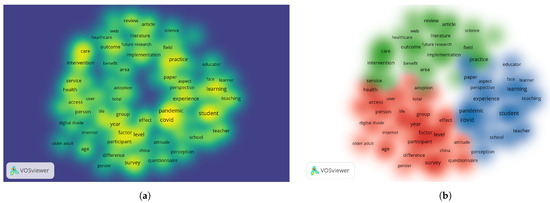
Figure 1.
The term occurrence map: (a) The term density. (b) The cluster organization.

Table 1.
Analysis of the top 9 obtained terms after the bibliographic study sorted by their relevance score.
The terms mentioned in the bibliographic study may suggest a concern for the education of older adults, with an emphasis on the process of learning and teaching, especially in the digital context of health and medical services.
2.3. Direct Observation Analysis
2.3.1. Usage of Digital Technology in Teaching
Recent developments in the digital technology field have led to changes in educational processes, starting with teaching. A greater importance is being given to the integration of all the components of the teaching process using specific architectures and concepts. One of the most fundamental components used is represented by learning management systems (LMS) that contribute to the organization of all educational processes for an institution or for a teacher. The accumulation of large sets of information on these systems leads to a need for analysis in order to develop the performance measurement of the educational processes. Thus, related to the teaching phase, the most important influences of digital technology are based on the usage of
- learning management systems (LMS) [17,18], that can integrate several components of the educational process;
- educational applications [19,20], used for the design, generation, storage and presentation of educational content;
- content management [21];
- educational experience development [22];
- video-based content [23] in the form of videoconferences or webinars.
2.3.2. Usage of Digital Technology in Learning
The process of learning is a complex one and is influenced by a large set of factors. The foundation of the learning process can be identified in psychological theories and biological processes from which several methods and techniques were developed. In order to design a better learning experience, digital methods and instruments are used on a large scale. The pervasive characteristic of the technology led to the development of the learning contexts both spatially and temporally, with the learning process having the potential to take place where the digital instruments are used (e.g., mobile learning is taking place where mobile devices are used). Thus, for the learning phase, one of the main challenges is related to
- pervasive learning [24] using mobile environments;
- adaptive learning systems [25];
- collaborative learning [26];
- gamification [27].
2.3.3. Usage of Digital Technology in Assessment
The objective of an educational process is the achievement of the main purposes established in its design phases. One of the main possibilities for achieving these objectives is related to an objective assessment. The objectivity of an assessment process is related to the appropriate design of assessment tools and the valid analysis of assessment results, which can be conceptually achieved by using specific pedagogical methods such as Universal Design for Learning (UDL) [28] or, more precisely, Universal Design for Assessment (UDA) [29], technically implemented using computational methods, such as machine learning, evolutionary algorithms and thoroughly studied using, for example, Learning Analytics (LA) [30] or statistical indicators [31,32]. The main objective of a successful automated design and analysis of an evaluation test is to be as close as a human-centered approach to a design result with similar requirements, because human experience is still difficult to overcome in terms of the test of specific assessment and article design and analysis [33]. The problematic elements that frequently appear in the general context of the evaluation can be considered:
- Creating a fair assessment for a group of students who were taught as a group. Equity refers to a fair distribution of balanced assessment items for each student within a group.
- The human errors that occur.
- Covering an extended area of previously learned subjects.
- The mix between practical and theoretical evaluation.
There is a wealth of literature on optimizing the evaluation process in terms of the design and analysis of evaluation components. Most of the area of automated educational assessment consists of developing models and assessment tools for Question Generation (QG) and Answer Evaluation (AE). An important part of the AE branch is devoted to Automatic Essay Scoring (AES), as shown in [34,35,36], which has been extensively researched in recent years. Regarding the QG branch, most research has been directed toward generating objective questions, such as multiple-choice ([37,38]), true-false [39] or open-ended questions ([40,41]). The classical topics of QG research are related to the formulation of questions from learning material, so recent research has been widely related to question sentence generation [42] and question generation from any type of text [43], including artificial intelligence [40]. To visualize the extent of research on this topic, empirical research on the subject of articles in scientific databases revealed that the topic is of wide interest in the research area. This research was carried out based on a search operation on specific keywords (for example, for the specific keyword “automated question generation”). Searching the Google Scholar paper database returned 292 unique results for 2022. Regarding the methods used to accomplish this task, one of the most used is Natural Language Processing (NLP), which was developed and perfected over time. For the AE branch, the research focuses on the analysis of short answers and essays, which also uses NLP-based techniques to perform a performant analysis of the text in the answer. One of the most researched topics is the assessment of answer correctness, especially related to a certain type of question (e.g., multiple-choice questions, as in [44,45]). However, a growing interest can be seen in the evaluation of automated responses to essay-type items ([46,47]). Another important part of research in educational evaluation is related to Item Analysis (IA), a field located at the border of several fields, such as statistics, psychometrics, evaluation, or education. It presents a wide range of research topics related to the mathematical and statistical aspects of assessment analysis [48], which remain benchmarks in the subject of item analysis and are heavily integrated into learning management systems as core functionalities for the human-centered analysis of educational activity on a specific platform. Item analysis is an extremely important method in studying student performance over given periods of time [49]. For these topics, two approaches are considered to be most appropriate for item analysis: Classical Test Theory (CTT) and Item Response Theory (IRT). While CTT uses statistical tools [50], such as proportions, means and correlations and is used for smaller-scale assessment contexts, IRT is a more recent development and is studied in relation to its more adaptive nature [51]. The adaptive character of the IRT method consists of the important consideration of the human factor related to the evaluation process. One of the most important differences between the two approaches is based on the assessee’s previous learning experience, as IRT creates an adaptive analysis based on a measurement precision that takes into account latent attribute values, while CTT starts from the assumption that this precision is equal for all individuals [52]. In this paper, tangential concepts are used to describe the development of a component of the model, especially regarding the statistical analysis of the items.
2.3.4. Review Summary
Table 2 presents a short excerpt highlighting the main methods and instruments used in key educational processes based on the review presented above.
Table 2.
Educational process phases, methods, and instruments.
In a further development of the research literature, an important field that has recently had serious practical implications in the educational process is Deep Knowledge Tracking [53]. It has gained a lot of exposure in the recent period of continuous development of online education due to the fact that it proposes the analysis and prediction of the student’s educational behavior based on personal previous learning experiences and assessments.
Despite the considerable progress in the integration of digital technology in education, several important research gaps remain:
- lack of real-time adaptive personalization: the majority of the research directions are related to the development of a standardized educational context, which is based on a determined non-variated educational content for all the participants of the educational process.
- emphasis on the integrative aspect of the educational process: The solutions often treat teaching, learning, and assessment as separate components, without integrating them into a system.
- Limited use of evolutionary optimization algorithms: The usage of AI and ML-based methods are extensive for the learning and assessment components, but the usage of heuristic algorithms, such as genetic methods, are under-explored.
- Lack of validation in real-world educational environments: The integration of models within educational tools is low, the described models being validated only through simulated data or theoretical models.
These gaps motivate the development of the proposed model, which aims to address the first three challenges directly while also laying the groundwork for future work in empirical validation and educational impact assessment, especially related to the latter point in the list.
Related to the selection of the genetic methods, the reasons of this selection are related to the nature of the problem to be solved. The generation of learning paths and assessment units are complex tasks. Both tasks involve combinatorial optimization, multi-criteria balancing, and continuous adaptation, making Genetic Algorithms (GAs) a suitable heuristic method.
Although the focus of the DMAIR model is on educational environments, we acknowledge the relevance of widely used optimization and control techniques in other domains, such as state-filtered disturbance rejection control, multilayer neurocontrol, and active disturbance rejection methods applied to nonlinear systems. These approaches provide valuable insights into handling uncertainty, adaptability, and system robustness and will be studied as potential implications within the model.
The main advantages of the GAs are related to flexibility in exploring large solution spaces, adaptability to multi-objective optimization and robustness in avoiding local optima. While GAs may require tuning and computation time, their ability to model nonlinear, adaptive educational scenarios justifies their use in this context.
3. DMAIR Description
3.1. General Considerations and Purpose
The model presented in this paper shows innovation aspects related to a complete overview of the learning process, starting from the teaching phase and continuing to the learning and assessment phases. In this matter, the Dynamic Model for Assessment and Interpretation of Results (DMAIR), developed sequentially and continually in [54,55,56,57], with various variations, such as in [58], shows a perspective of integrating automated tasks in the educational process. This initiative would reduce the effort generated by human-made educational tasks. At the same time, its mechanisms should replicate the human expertise related to process quality in teaching, learning and assessment (TLA) as close as possible. The model responses to the specific research gaps identified earlier by the following:
- Dynamic personalization: The learning process, emphasized by the learning path generation, and the assessment component, related to assessment test generation, carry a high potential for learning personalization.
- An integrated model for adaptive learning: The proposed model offers a unified framework that connects the teaching, learning, and assessment processes.
- Usage of genetic algorithms: Based on specific elements of Classical Test Theory and Item Response Theory, among other theoretical frameworks, for a valid scientific foundation of the model design, the advantages of the solutions of the genetic algorithms are explored.
- scalable architecture: the model is designed with flexibility in mind, following a scalability-driven structure and taking into account the future integration into existing and developing Learning Management Systems.
These contributions address the first three research gaps directly. While real-world validations are only partially addressed in this stage, the proposed architecture establishes a solid foundation for future experimental studies in authentic educational environments.
The main innovative aspects that show novelty related to existent approaches are related to the following:
- The interaction between the learning and teaching component and the assessment component, both using dynamic evolutionary-based methods to obtain the desired results;
- the traditional approaches related to learning path generation are related to rule-based approaches or static branching logic. In this matter, the current model uses genetic algorithms to optimize the structure and sequence of learning blocks for each learner;
- the integration of a closed feedback loop by integrating automated generation, real-time analysis, and interpretation of results related to assessment;
- the accent is put on the optimization of the learning and assessment process with a direct influence on learning progression; the model adapts both what is taught and how learners are assessed;
- the architecture of the model is a modular one, with the scalability and integration of the implementation in specific learning platforms in mind.
To ensure computational feasibility when applying genetic algorithms in large-scale environments, the model supports parallel processing strategies and can be integrated with distributed computing infrastructures such as cloud-based platforms. Also, optimization techniques such as genetic parameter tuning and population variation are studied to address scalability related to high volumes of data.
An educational scenario may take into account an online platform designed to teach high school biology. A student logs in to begin a new unit on genetics. The model first generates a diagnostic assessment with varied difficulty levels and topics. Based on the student’s responses, a personalized sequence of learning blocks is generated, including video lessons, interactive quizzes, simulations, and reading assignments, arranged to address weak points and reinforce core concepts.
As the student progresses, the model continuously monitors performance through embedded micro-assessments. At the end of the unit, a summative test is generated and adapted in real-time based on prior performance, ensuring both fairness and relevance.
The design of the DMAIR model is grounded in key educational principles that support its integration into modern teaching practices. The system aligns with constructivist learning theory, as it facilitates individualized knowledge construction through modular learning blocks tailored to each student’s prior performance. The continuous feedback loop between assessment and content delivery also reflects the principles of formative assessment, enabling instruction to be adjusted in real time based on learner needs. From an implementation perspective, DMAIR has been conceived as a modular and LMS-compatible tool. Thus, the model ensures the alignment with theoretical and implementation frameworks related to pedagogical theory.
3.2. Learning and Teaching (LT)
3.2.1. General Considerations and Purpose
Related to the learning and teaching components of the educational process, the most usual element used as a unit of encapsulation for adapting the processes to digital technology is stated to be a learning object or a learning block. This section presents the model used for the development of learning blocks to design learning paths. The design process of a block path requires organizational skills. This process has characteristics that permit its usage within education process planning, which is very important within the context of adaptive learning systems. The purpose of the implementation of the LT model component consists of the development of a learning path that follows the requirements of an initial and final learning block, aligned with the desired objectives: (1) learning path length/duration and (2) learning path depth/order of generality. Thus, the next elements are given for this issue:
- Context input: a set of learning blocks described by the concepts that are needed for learning each block are given.
- Desired output: a learning path that would respect specific criteria based on start and end concepts, duration and order of generality are requested.
A general idea of solving this issue would be the determination of connections between blocks using a genetic algorithm. Using the connections between the blocks, a matrix with the best configuration of connection is generated using a genetic algorithm. In this matrix, the connections between learning blocks from general to particular are made based on an ontology of concepts, which organizes the concepts in an arborescent form. From these matrices, an optimal learning path is obtained based on specific criteria. Similar concepts were firstly described in our research in ([59,60,61]).
3.2.2. LT Component Structure
Learning Structures
In order to create the desired learning paths formed of the learning blocks, the most important structures that will be used in this approach are the ontology of concepts (O), the learning block (B), the block relationship (), the block matrix () and the learning path (), presented as follows:
- O is an ontology of concepts, which is a structured set of semantic tags related by a hierarchic relationship. It can be represented as a graph or as a symbolic logic structure. In this paper, an ontology is a directed graph of concepts:where
- -
- is the set of concepts that can be determined using an automated method of extracting concepts from a corpus of text (e.g., using Natural Language Processing);
- -
- is the set of edges, where an edge defines a hierarchical relationship between two concepts;
- B is the learning block, which is the most basic unit of learning. A block is a quintuple of elements, codified as follows:where
- -
- is the set of keywords that define the prerequisite concepts, i.e., the concepts needed to be known in order to follow the current learning block;
- -
- is the set of keywords that define the concepts learnt in the current learning block;
- -
- is the set of semantic tags that reflects the upper level in a digital ontology of concepts that describe the learning block;
- -
- is the set of semantic tags that reflects the lower level in a digital ontology of concepts that describe the learning block;
- -
- P is the ensemble of learning processes, methods, instruments, and elements needed in the learning process run in the current learning block.
A graphical representation of a learning block is shown in Figure 2. We can observe that the elements of and sets are represented as sockets that can be connected with similar ones. Also, a block is characterized by a level in a correspondent ontology of concepts that is formed based on the set of blocks and delimited by an upper level (concepts that are more general than the ones studied in the current block) and by a lower level (concepts that are more particular or detailed than the one studied in the current block). The colours are expressed in order to differentiate easier between the elements of the block.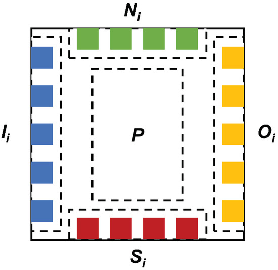 Figure 2. The graphical representation of a learning block.
 - is the block relationship established between two blocks, which can be differentiated into two types:
- -
- linear, , which is established between two blocks situated on the same ontology level, based on the keywords matching. The connection can be made if the output keywords of the first block are fully or partially matched with the input keywords of the second block:
- -
- leveled, , which is established between two blocks situated on neighboring levels related to a specific ontology, based on the sets of semantic tags. The connection can be made if the current semantic tag of the first block is connected in the ontology O with the semantic tag of the second block:
- is the bidimensional array or matrix that contains a specific configuration of a set of learning blocks. A bidimensional array is a structure formed of learning blocks that may be connected based on the four edges of a block:A matrix is obtained as a result of a genetic algorithm that will be described in the next sections. In this context, L(O) represents the number of levels within the generated ontology (O).
- is a learning path, a successive enumeration of blocks that start with an initial block BS and ends with a final block . A path contains only blocks that are connected either linearly or leveled:
The requirements given for the determination of the best learning path are classified in two phases:
- The requirements for the determination of the best are as follows:
- -
- R1: the matrix contains the and learning blocks;
- -
- R2: the matrix has the highest number of connections between the forming blocks;
- -
- R3: the matrix has a generality index () as close as a value given by the user (), where the generality index is the ratio between the column index of the block in the determined and .
- The requirements for the determination of the best are as follows:
- -
- R4: the path is the optimal path between the and learning blocks, where optimal may consist of the minimum or the maximum steps in the matrix, according to the user requirement;
- -
- R5: the path has the “lowest” block (i.e., lowest refers to the maximum index of the matrix lines where a block from is found) as close as .
Genetic Structures
In order to determine the best , a genetic algorithm will be applied. Thus, the main genetic structures are determined as follows:
- g is the gene of a genetic algorithm and codifies a given block in the bidimensional array:
- C is a chromosome and codifies a bidimensional array, which can be structured as an unfolded unidimensional array of :
- P is the parameter set of the genetic algorithm, a quadruple of variables which defines the set of the genetic algorithm parameters, , where is the initial population size, the number of generations, the mutation rate and the crossover rate, , .
- is the fitness function, defined as the maximum number of valid connections between the blocks within the chromosome, as follows:where
- -
- defines the R1 requirement;
- -
- defines the R2 requirements based on relationships;
- -
- defines the R2 requirements based on relationships;
- -
- defines the R3 requirement.
The measure of the total value of the fitness function over the interval [0, 1] is ensured.
Genetic Operators
Genetic operators are mutation, crossover and selection, described as follows:
- Mutation (Mut), represented by the replacement of a randomly-selected gene with a randomly-chosen block in a randomly-chosen position;
- Crossover (Crs), determined between two parent chromosomes C1 and C2. A common random position for both chromosomes is generated. The chromosomes are split by the position. The first part of the C1 chromosome is combined with the second part of the chromosome C2 and the first part of the chromosome C2 is combined with the second part of the chromosome C1. Two offspring chromosomes are obtained;
- Selection (Sel), represented by the sort operation of the chromosome by the fitness function value.
3.2.3. LT Component Functionality
Genetic Algorithms
For the genetic algorithm methodology, which outputs the best BM, the next steps are applied:
- Step 1:
- The input data (B set, BS, BE, P, uGP) is read.
- Step 2:
- The genetic algorithm is applied as follows:
- (a)
- the generation of the initial population of items is made;
- (b)
- the mutation operation is applied;
- (c)
- the crossover operation is applied;
- (d)
- the resulted chromosomes are selected;
- (e)
- after NG generations, the best chromosome is selected.
- Step 3:
- The best chromosome is input.
Matrices Algorithms
The algorithm related to finding the best BLP can be assessed using specific algorithms. For example, for finding the shortest path, Lee’s Algorithm can be applied. As for the longest path, a BFS search can be made in the BM matrix. For both the cases, an additional requirement (R5) is verified. For finding the shortest path, the algorithm may follow the next steps:
- Step 1:
- Initialize:
- (a)
- Initialize a queue to store cells to explore.
- (b)
- Mark the start cell as visited and add it to the queue.
- (c)
- Initialize the current level to 0.
- Step 2:
- Explore and expand:
- (a)
- While the queue is not empty:
- Increment the current level.
- Determine the number of cells at the current level.
- For each cell at the current level:
- Check if this cell is the end cell.
- If it is, return the current level (indicating the shortest path is found).
- Otherwise, for each unvisited neighbor cell:
- Mark the neighbor as visited.
- Enqueue the neighbor to the queue.
- Step 3:
- Update queue: Remove all cells at the current level from the queue.
- Step 4:
- Termination: If no path is found, return a message indicating that there is no path between the start and end cells.
3.3. Assessment–Test Generation (TG)
3.3.1. General Considerations and Purpose
The DMAIR model comprises several components that are essential to an assessment system. This system must consist of three main functionalities: item generation (func1 (I)), verification mechanisms (func2 (II)) and response evaluation (func3 (III)). A graphical representation of the model is shown in Figure 3.
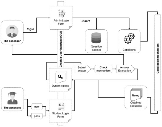
Figure 3.
The main schematic representation of the assessment model.
In this matter, the general purpose of the model is to obtain a specific assessment test (configuration of items) starting from a set of assessment items (questions, exercises, etc.) of N cardinality, which is established during an undefined period of time or automatically generated using specific methods (e.g., NLP). The test is generated taking into account specific requirements, such as the total solving time of the test, the subject of the items within the test, the degree of difficulty, etc. For the generation process, evolutionary-based methods are applied.
3.3.2. TG Component Structure
Assessment Structures
The main elements used in the generation process are the item (q), the sequence of items or the test () and the requirements (R), described as follows:
- q: the item, a tuple , generated and stored in a database, where the elements of the tuple are as follows:
- -
- : the unique identification particle of the item;
- -
- : the statement, which consists of a phrase or set of phrases that describes the initial data and item requests to be resolved;
- -
- : the number of keywords that define an item;
- -
- : the set of keywords, considered similar to a semantic tag, represents a collection of keywords defining an item. A keyword, denoted as , refers to a term or phrase that characterizes the subject matter of the item. These keywords can be acquired either manually by a human operator or automatically through Machine Learning (ML) powered Natural Language Processing (NLP) methodologies;
- -
- : the degree of difficulty of the item, determined through specific metrics (typically statistical, such as the ratio between the number of correct responses to the item and the total number of attempts or responses);
- -
- : the item type, where m has the meaning of multiple-choice item, e essay item and s short-answer item;
- -
- (where necessary): a list of two or more possible answers when the item type is multiple or null or when the item type is short or essay;
- -
- : the theoretical or practical nature of the item, where 0 is theoretical and 1 is practical.
- SI: the sequence of items, a tuple that encodes an educational assessment test created according to specified criteria or requirements using genetic algorithms. The components of the tuple are as follows:
- -
- : the unique identification particle of the test;
- -
- : the test size (the number of questions);
- -
- : the set of items that form the test;
- -
- : the union of the sets of keywords of all the items q within the sequence;
- -
- : the degree of difficulty of the item, which is calculated as an average of the degrees of difficulty of all the items that form a test, as follows:
- -
- : the theoretical-practical ratio, which gives the predominant type of SI, the value of the ratio consisting of the proportion of theoretical questions and the difference 1 – TP being the proportion of practical questions;
- -
- : an array determining the predominant item type in SI. The values of the vector contain the number of items of each type in SI, being the number of multiple-choice items, being the number of short-type items, and being the number of essay-type items.
- R: the set of requirements , where is a requirement for the test generation and k the total number of requirements. For this paper, or and the requirements are as follows:
- -
- represents the requirement associated with the topic of the items required in the sequence. This requirement is linked to the set of user-desired keywords, denoted as , where represents the list of user-defined keywords and represents their total count;
- -
- is the requirement related to the degree of difficulty. is related to the desired degree of difficulty, where , a value closer to zero means that the test is desired to be “less difficult” and closer to 1 being “more difficult”;
- -
- is the requirement related to the predominant item type, which can take values from the type set; thus, ;
- -
- is the requirement related to the desired theoretical/practical ratio ().
Arborescent Structures
The usage of a network-type structure (Figure 4) is useful in the situation where the aim is to generate a sequence of items SI given the membership of the items in the taxonomic framework of a subject. In this sense, modeling is reduced to the formation of a network between the generated items, between which a hierarchical relationship is established, depending on their taxonomic classification or sequential degree of difficulty. The numbers in Figure 4a,b represent the identification particles of the items.
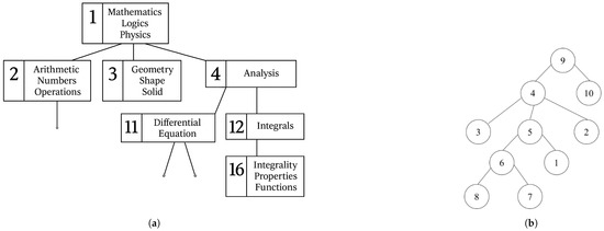
Figure 4.
Representations of sequences of items as graphs: (a) structures with keywords (b) structures with identification particles.
Given such a representation of items, the problem of this description reduces to finding a partial tree between the root node and any leaf node. The root has the lowest degree of difficulty (so it is the least difficult item) and the leaves are the most difficult items. The output of the model is a sequence of items that satisfies two conditions:
- forms a partial tree of the main tree;
- the number of missing edges between nodes in the generated subtree is zero or minimal, based on the connections in the main tree (the tree is connected);
- the generated tree contains items whose cardinal of the reunion of sets of keywords within the tree is the closest as the number of keywords desired by the user.
The tree that codifies a sequence of items can be generated by various methods. The ones used in previous research are direct searches (BFS or DFS) and genetic algorithms. The main arborescent structures used to generate an SI are the graph (G), the subgraph (T) that codifies the sequence of items SI, the set of parameters (P) and the fitness function (h) for the genetic approach, described as follows:
- : the undirected graph that represents the items and the relationships between them. The set of vertices or nodes contains the items in the database and the set of edges contains all the conceptual relationships between the items, determined based on the ontology of concepts (O);
- : the subgraph generated by various methods. The set of vertices or nodes contains the selected items to be part of an SI and the set of edges contains all the conceptual relationships between the items in the SI, based on the graph G.
- P: a quadruple of variables which defines the set of the genetic algorithm parameters, , where NP is the initial population size, NG the number of generations, rm the mutation rate and rc the crossover rate, ;
- is the fitness function that verifies that the generated subgraph is connected, is a tree and contains the keywords given by the user. Thus, it combines the two given requirements described above
Genetic Structures
The main genetic structures used to generate an SI are the gene (g), the chromosome (C), the set of parameters (P) and the fitness function (f), described as follows:
- : the gene, which encodes the items , within a test;
- : the chromosome which encodes a sequence of items SI;
- P: a quadruple of variables which defines the set of the genetic algorithm parameters, , where NP is the initial population size, NG the number of generations, rm the mutation rate and rc the crossover rate, ;
- : the fitness function, defined in various stages depending on the requirements. Two forms used in various papers are presented:
- -
- as an average value of several sigmoid functions, as follows:where and are the specific values of the function given by each parameter, as follows:
- *
- is related to the number of common keywords between the SI and the desired keywords;
- *
- is the keyword coverage of the SI. It measures the proportion of the uKW keywords in the sequence;
- *
- is the inverse of the dispersion of the variation of user-defined keyword frequencies throughout the sequence (the balance of the keywords within the sequence);
- *
- is the inverse value of the absolute difference between the desired degree of difficulty and the sequence one;
- *
- defines the predominant type of item, where is the frequency of the user-defined item type in the sequence.
- -
- As a sum of various functions. This form has the next description:In short, the fitness function calculates the value of the average of all constraints as follows:
- *
- the highest average value of similarity between user-given keywords and item keywords, calculated using edit distance and specific NLP methods;
- *
- the smallest value of the difference between the desired degree of difficulty (uD) and the calculated degree of difficulty (D) for SI;
- *
- the smallest value of the difference between the desired theoretical/practical ratio (uTP) and calculated for SI;
- *
- the smallest value of the sum of the differences between the components of the desired vector values () and calculated for the SI that describes the predominant type of item.
Genetic Operators
The genetic operators are established to be common with the ones presented in the LT component structure: the mutation (Mut), the crossover (Crs) and the Selection (Sel).
3.3.3. TG Component Functionality–func1(I)
For the genetic algorithm methodology, which outputs the best SI, the next steps are applied:
- Step 1:
- The input data (q set, uD, uTP, P, kw set, nKW) are read.
- Step 2:
- The genetic algorithm is applied as follows:
- (a)
- the generation of the initial population of items is made;
- (b)
- the mutation operation is applied;
- (c)
- the crossover operation is applied;
- (d)
- the resulted chromosomes are selected;
- (e)
- after NG generations, the best chromosome is selected.
- Step 3:
- The best chromosome is input.
As for the approach using arborescent structures, the next approach is used:
- Step 1:
- The initial set of items is constructed, either retrieved from a database or generated from a corpus.
- Step 2:
- A tree containing a relational structure of items is created based on Automatic Taxonomy Construction (ATC) and/or sequential difficulty.
- Step 3:
- The leaf nodes and their number are determined, their values being stored in the leaf array. In a simplified scheme, the determination is made as follows:
- Step 4:
- Using the values determined in step 3, the leaf-to-node sequences are constructed starting from the leaves to the root and the nodes are stored in an array L.
- Step 4:
- Within the sequence, we determine the number of keywords that appear in it and the number of occurrences of the keyword in the sequence.
- Step 5:
- The sequence with the maximum number of keywords is determined and found. The output values are the sequence and number of occurrences of each set keyword.
3.4. Assessment–func2(II) (Check Mechanism–CM)
This component of the model includes checking user responses to items generated within other components. In the case of multiple-choice items, this automatic verification of answers is a trivial process, accomplished by comparing the answers given by the respondents to the item with the correct answers to the item.
For the other two types of items considered in the model, checking the answers is a complex aspect, given the nature of the answers. In this sense, the purpose of the model component is to achieve an automatic verification as close as possible by a human user, and this can currently be achieved using specific Machine Learning (ML) methods developed in the specialized literature, based on processing natural language processing (NLP).
Next, we want to describe an attempt to establish an automatic check for short open-ended answers made in a previous work, which uses edit distance to determine the degree of similarity between two answers. To define the degree of similarity between two answers given to the same question, we will consider the answers as strings. They will be denoted by R1 and R2. To calculate the degree of similarity, we will remove from R and R2 the characters that belong to a set M (characters such as space, tab, new line, punctuation marks, etc.). After this operation, two more strings, denoted T1 and T2, will result.
To calculate this edit distance, there is an O(m × n) complexity algorithm, where m is the number of characters in T1 and n is the number of characters in T2. This algorithm uses the dynamic programming method and is based on the following recurrence formulas ([62]):
where is the edit distance for the sequence consisting of the first i characters in T1 and the sequence consisting of the first j characters in T2. The edit distance between T1 and T2 is d(m,n). Thus, the similarity degree is presented in Equation (15).
3.5. Assessment–func3(III) (Item Analysis–IA)
The func3 component (III), described in detail in [63,64] and whose schematic representation is shown in Figure 5, is designed based on the premise that an incorrect answer to an item may indicate that the topic of the item is not fully understood, especially under certain conditions (e.g., other items in SI are answered correctly for a student answer, the item repeatedly gets wrong answers for several students, etc.). The model takes into account several factors to determine the direct causality between poor understanding of the subject and the incorrect response to an item with that subject. The main components of the IA component are as follows:
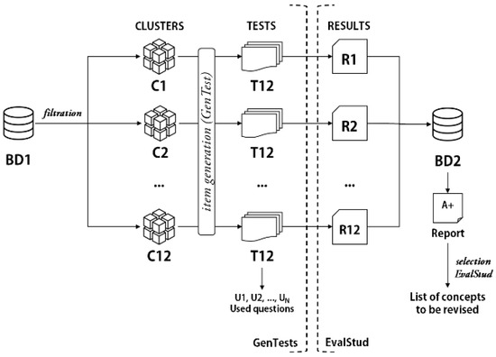
Figure 5.
The general schematic representation of the Item Analysis model.
- q: the item, described in the previous subsection, but with some additional statistical features;
- : the sequence of items, also described in the previous subsection, which will be enriched with more statistical indicators;
- : student results, which contains information related to the assessment results of a particular student;
- G: the result of the group of students, which contains statistical information related to the results of the assessment of a certain group of students (for example, class, group).
The func3(III) algorithm consists of the following steps:
- Step 1:
- Students connect and solve the item sequences.
- Step 2:
- For each student and a specific sequence of items, a report is generated, created by following the following steps:
- (a)
- Elements that obtained lower values of mq (the average score of an item q) and lq (the number of correct answers to the item q) are filtered out.
- (b)
- The item parameter values dq (the discrimination index of the item q), pbsq (the biserial point of the item q), taq (the number of students who answered the item q), ddq (the degree of difficulty of the item q), uD and tsS (the total score of a student in the items of the same subject) are checked.
- (c)
- Item subjects are then extracted and verified to have obtained lower values for mq and lq in other items with the same subject for a large number of students.
- Step 3:
- The subjects of the items that validate the rule are presented in substep 2c).
- Step 4:
- The reports are entered into a report dataset, hereafter referred to as BD2.
A schematic approach to this algorithm is presented in the code presented in Algorithm 1.
| Algorithm 1 IA approach algorithm |
|
4. Results
4.1. General Methodology
Although the process of obtaining research results was made on specific components, based on the model implementation steps, this process has similar approaches and contained specific steps:
- Step 1:
- The definition of objectives and purpose: The main purposes were related to model simulations in a laboratory or real environment using several methods (direct observation, comparison, etc.).
- Step 2:
- The implementation of the model
- (a)
- Application design: the application design comprised the choice of the optimal application development environment (web, mobile, desktop, etc.) and the instruments used (formal modeling languages and techniques, programming languages, methods, architectures, frameworks, etc.);
- (b)
- Application development: the development consisted in the actual implementation of the model based on the blueprint design obtained at the previous step;
- (c)
- Testing and troubleshooting: the testing phase consisted in the calibration of the obtained instruments and the identification of specific errors or miscalculations.
- (d)
- Application integration and launching: the integration consisted of the connection action of the resulted implementation in a common learning framework. The launching aspects were related to the dissemination of implementation and its usage in data collection for various research contexts.
- Step 3:
- Data collection
- (a)
- The definition of objectives: the main purposes were related to the model validation using domain-specific methods, general (direct observation, comparison, etc.) or statistical;
- (b)
- Data collection: the data collection consisted of obtaining information based on the implementation behavior or specific research contexts;
- (c)
- Data pre-processing: In order to apply several instruments of methods, in several cases a pre-processing was necessary.
- Step 4:
- Data analysis: the collected data were analyzed to assess the achievement of the objectives and to test the formulated hypotheses. This analysis involved the use of statistical or analytical techniques to identify patterns, relationships, or trends in the collected data.
- Step 5:
- Data interpretation: The results of the analysis were interpreted in the context of previously established objectives and assumptions. The assessment was related to whether or not the data collected supported the hypotheses formulated and to identify the implications of these results for the implementation and the model theoretical assumptions.
In the context of the DMAIR model, we address potential concerns related to data privacy, algorithmic transparency, and learner autonomy. All learner data used in simulations are anonymized, and the model is designed to operate within GDPR-compliant frameworks when deployed in real-world scenarios. To mitigate algorithmic bias, DMAIR supports teacher oversight and manual review of generated assessments. The personalization process remains interpretable, allowing educators to understand and intervene in the learning path when necessary.
In the current experimental stage, the DMAIR model has been tested using synthetically generated datasets. These datasets were constructed to simulate realistic educational scenarios, including diverse learner profiles, varied item characteristics (datasets with items from various sources, human and machine-generated items and with various randomly-generated numerical indicators), and heterogeneous learning behaviors. The primary goal of using synthetic data was to validate the internal logic, adaptability, and optimization capacity of the model under controlled but meaningful conditions. While we acknowledge the limitations of simulation-based validation, the structure and parameterization of the datasets were designed to reflect the real world as closely as possible.
For a better pedagogical assessment of the model, some indicators related to this will be studied in future directions. Table 3 summarizes the main indicators and their corresponding purposes.
Table 3.
Educational performance indicators proposed for future validation.
These indicators will be central to future empirical validations of DMAIR, providing a more comprehensive understanding of the system’s educational impact and practical relevance.
4.2. Learning and Teaching-LT
We will show a short example of a model development, with the implementation being planned for further research. The next sets and their corresponding IDs were used for the keywords:
- for the levels: 1-fundamentals, 2-algorithms, 3-programming, 4-advanced_techniques, and 5-applications;
- for the inputs and outputs: 1-Data types, 2-Operations, 3-Structures, 4-Algorithms, 5-Searching, 6-Sorting, 7-Functions, 8-Recursion, 9-OOP, 10-Threads, 11-Databases, 12-SQL, 13-Web, 14-JavaScript, and 15-APIs.
The characteristics of the blocks taken as example are shown in Table 4 and an example of a simulated generated BM matrix is shown in Table 5. The algorithm would next find the best using a search algorithm in the matrix (e.g., Lee).
Table 4.
The characteristics of the blocks.
Table 5.
Example of generated BM matrix.
4.3. Assessment–Test Generation (TG)
4.3.1. TG Using Arborescent Structures
Related to test generation using arborescent structures, we have determined two simulations related to a specific topic and run several trials for the model presented in previous sections. The purpose of the implementation was the determination of the algorithm workflow and its behavior in a simulation environment.
In the first implementation, based on the Python 3.12 programming language, a number of nodes and their characteristics was randomly generated. In the technical setup, a tree with 100 nodes is generated, each with a random set of keywords and a difficulty between 1 and 10. Nodes are randomly connected with a probability of 30%, but only if the difficulty of the child node is higher than that of the parent. The selected keyword set is {“array”, “path”, “loop”, “prime”, “query”, “bfs”}. The structure of the tree and the resulted subtree, with the selected items shown in green, are presented in Figure 6.
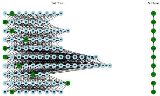
Figure 6.
The visual representation of the arborescent structures for the implementation.
The results show a subtree selected based on the desired keywords, with a maximum number of intersections (nine keywords) and eight valid edges from the original tree. Table 6 displays, for each node the level, ID, keywords, and number of intersections with the desired words.
Table 6.
The chosen items and their characteristics.
The algorithm is efficient due to the selection of nodes by difficulty levels and the use of a score based on the intersection of keywords. With nine intersections and eight valid edges for the given example, it shows how it minimizes the computational time by quickly evaluating relevant nodes and existing connections.
In the second implementation, a database closer to real items were made. The item topics are related to IT and computer concepts. The input variables are as follows:
- the number of nodes (the total number of items) equal to 35;
- the initial graph in form of a tree, given by the parent array t = (0, 1, 1, 2, 15, 15, 3, 3, 4, 4, 4, 4, 9, 25, 2, 10, 11, 11, 12, 7, 7, 8, 8, 8, 8, 5, 5, 6, 6, 20, 20, 21, 22, 23, 24);
- the keywords given by the user = (hardware, PC, hard disk, memory, unit, external, reading, peripheral, software, application, browser, Internet).
The tree that can be built with the data presented above and all the keywords related to the nodes is shown in Figure 7.
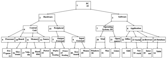
Figure 7.
The visual representation of the arborescent structure for the implementation.
After the run, several outcomes were determined related to potential tests. In order to determine the optimal ones, the model functionality was implemented. After the implementation was run, the next outcome was obtained (L contains the final output and the first element of the array is the array dimension):
- L = (5,1,2,4,11,18)-hardware 1 times; PC 1 times; harddisk 1 times; memory 1 times; unit 1 times;
- L = (5,1,2,15,5,27)-hardware 1 times; PC 1 times; external 1 times; reading 1 times; peripheral 1 times;
- L = (5,1,2,15,6,29)-hardware 1 times; PC 1 times; external 1 times; reading 1 times; peripheral 1 times;
- L = (5,1,3,8,25,36)-PC 1 times; software 1 times; application 1 times; browser 1 times; Internet 1 times.
4.3.2. TG Using Genetic Structures
Related to test generation using genetic structures, we have determined two simulations related to a specific topic and run several trials for the model presented in previous sections.
The first implementation was made in a laboratory-simulated experiment with randomly generated items and characteristics. The technical setup involved using a genetic algorithm to select and optimize a set of questions, with the goal of achieving an average difficulty of 0.4 and ensuring coverage of the desired keywords: {“python”, “algorithm”, “data”, “machine”, “learning”}. The algorithm operated with a population of 10 chromosomes (question sets), evolving for 50 generations, with a mutation rate of 0.1, to maximize fitness in relation to keyword difficulty and coverage. The evolution of the fitness values for the example is shown in Figure 8.
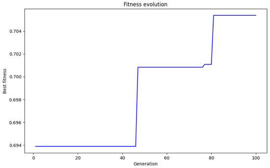
Figure 8.
The evolution of fitness value throughout the generations for the given example.
The genetic algorithm achieved a running time of 0.19 s and a final fitness of 0.7054, improving the previous result (0.6961). The best chromosome was [74, 101, 465, 704, 662, 368, 582, 45, 117, 271], with an average difficulty of 0.4170. The statistics related to the best chromosome are shown in Table 7.
Table 7.
The questions associated with the best chromosome.
The second implementation (Figure 9) was made as a web application using PHP scripting language for the backend, MySQL for the database component and the Laravel framework for the application model implementation, which uses an MVC architecture in order to take into account the scalability. Also, the set was closer to a real one.
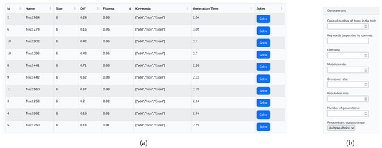
Figure 9.
Aspects of the GUI interface of the genetic-based method implementation: (a) test generation history (b) input data form.
In order to assess the efficiency of the genetic algorithm, several runs of the implementation were made. The purpose of the result analysis was the direct observation of the fitness compared to an initial random generated test. Additionally, the genetic population was measured using a specific metric: the population variation, showing how the population varies after the genetic operators are applied and the performance of the genetic algorithm. The initial data used for the runs were the following:
- the number of items in the database (N) was 800;
- the number of desired items in the sequence (m) was 10;
- three keywords were chosen (uKW = 3);
- a degree of difficulty of 0.4 was chosen (uD = 0.4);
- the desired type of question was chosen as multiple-choice (uT = ′m′);
- the mutation rate was established at 0.1 (rm = 0.1);
- the crossover rate was established at 0.5 (rc = 0.5);
- the population size was established at 50 (NP = 50);
- the number of generations was established at 100 (NG = 100);
- the fitness function is the sigmoid average.
The obtained data after the implementation are presented in Table 8.
Table 8.
Obtained data after the genetic-based implementation.
Regarding the efficiency of the algorithm, one of the quantitative indicators is the run time related to the parameters of the genetic algorithm. The parameters that were considered to influence the run time were N (the number of questions), K (the number of questions within a test) and NG (the number of generations of genetic algorithms). The tests were conducted in a Java-based implementation on a system with the following parameters: a Windows 8 operating system, an i3-3217U 1.80 GHz microprocessor and 4GB RAM. The results are shown in Table 9 and are compared with the previous results of previous versions of genetic algorithms.
Table 9.
Runtime data after the genetic-based implementation.
The running time of the genetic algorithm is significantly influenced by the parameters of the experiment, such as the population size and the number of generations. The larger the population or the number of generations, the longer the running time, because the algorithm requires more iterations to evaluate and optimize the solutions. The complexity of the genetic algorithm is generally , where NG is the number of generations, P is the population size and K is the number of items desired in a test. This means that the algorithm becomes slower as the population size or the number of generations increases, and the running time will increase significantly for large datasets. Compared to a previous algorithm, the current implementation demonstrated a shorter running time, which suggests a performance optimization, but the same principles of complexity apply. The parameters must be chosen carefully to balance the running time and the quality of the solutions.
In order to express the correlations between the three parameters (N, K and NG) and their combined and individual influence on the runtime, we have designed, implemented and run a multiple linear regression model. The setup of this model was performed using the Ordinary Least Squares (OLS) technique to estimate the coefficients of a linear function describing the relationship between the independent variables N (number of items), K (number of items per test), and NG (number of generations), and the dependent variable Runtime (execution time). The algorithm was implemented on a training dataset, and the model was trained to minimize the sum of squared errors between the predicted and actual values of Runtime. Error measures such as MSE (Mean Squared Error), RMSE (Root Mean Squared Error), and were used to evaluate the performance. Thus, the regression function has the next form:
where
- is the intercept (the constant term),
- , , and are the coefficients that determine the influence of each variable (N, K, NG) on Runtime.
The linear regression model scored well in the performance evaluation, with an MSE of 0.331 and an RMSE of 0.576, indicating a relatively low mean error. The MAE is 0.429, suggesting that the mean absolute error is quite small, and the MAPE is 0.045, meaning a very low mean percentage error. With an of 0.975, the model explains 97.5% of the variability in the data, indicating excellent performance.
The coefficients obtained for each feature, such as N (coefficient 0.000921372), K (coefficient 1.87163 × 10⁻⁵), and NG (coefficient 0.0118544), indicate the influence of each variable on runtime, and the intercept (−0.19403) represents the estimated value of Runtime when all predictors are zero. This setup ensures the estimation of a regression model capable of predicting runtime based on the specified inputs. The plots related to the dependency of N, K and NG on the runtime are shown in Figure 10a–c.
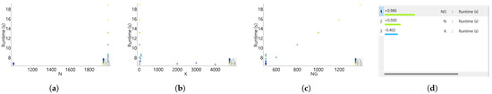
Figure 10.
The influence of each parameter (N, K and NG) on the runtime of the algorithm: (a) N (b) K (c) NG (d) individual correlation.
The estimated function is a linear regression that models the relationship between the explanatory variables (N, K, NG) and the algorithm’s runtime (Runtime). The intercept coefficient (−0.19403) represents the estimated runtime when all other variables are zero. The coefficient for N (0.000921372) suggests that for every unit increase in N, the runtime increases by approximately 0.00092 s. The coefficient for K (1.87163 × 10⁻⁵) is much smaller, indicating a minor influence on the runtime compared to N and NG, with a very small increase in runtime for each unit increase in K. In contrast, the coefficient for NG (0.0118544) indicates a significant influence, suggesting that an increase in the value of NG has a much larger impact on runtime, with an increase of approximately 0.01185 s for each unit added in NG. Thus, it can be concluded that NG has the largest impact on performance (runtime), followed by N, and K has a smaller influence.
The indicated Pearson coefficients (Figure 10d) suggest different relationships between the independent variables and the execution time. The very strong and positive correlation (+0.986) between NG (number of generations) and Runtime suggests that as NG increases, the execution time tends to increase significantly. The moderately positive relationship (+0.500) between N (number of items) and Runtime indicates a less strong, but still significant, influence on the increase in execution time as N increases. In contrast, the negative correlation (−0.402) between K (number of items per test) and Runtime suggests that as K increases, the execution time decreases, indicating a possible increased efficiency in the case of tests with more items.
Considering the hardware system used, the results indicate that the genetic algorithm can work efficiently even on a less powerful platform, but the complexity can significantly affect the performance on large datasets or for long-running executions. In such cases, further optimization of the algorithm or more powerful hardware may be required to avoid an excessive increase in runtime. Therefore, finding an optimal balance between the algorithm parameters, its complexity and the available hardware resources is essential to obtain quality solutions in a reasonable time.
The results show that the most influential parameter of the genetic algorithm for item generation is the number of generations. The significant increase is offset by the smoother results obtained after running a larger number of generations.
4.4. Assessment–Item Analysis (IA)
In order to assess the workflow of the Item Analysis component, an implementation in the form of a web application (Figure 11) was established. The implementation was made using the PHP web programming language, and the interface was created using the Bootstrap library, which is based on HTML, CSS and JavaScript languages. Then, the model was tested based on a focus group context. The initial context was considered to be a group of 20 students who attended an ICT course over a period of one semester (14 weeks) and a total of five tests were taken during this period. Each test was generated to contain five questions with specific topics related to the use of various applications (Word, Excel) or notions related to the Internet, programming and operating systems. The type of all questions was multiple choice.
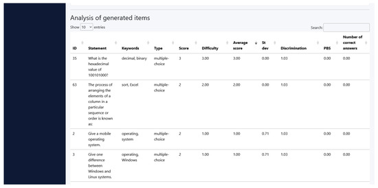
Figure 11.
A GUI screenshot of the Item Analysis implementation.
For the items described in the initial data analysis, the responses were analyzed by determining the values of the model parameters considered. For this specific example, the score was equal to the number of correct answers due to the fact that each question was scored with 1 point. The results are presented in Table 10. The columns presented in Table 10 show the degree of difficulty (dd_q), standard deviation (sd_q), item discrimination (d_q), point-biserial (pbs_q), mean score (m_q), and the number of correct answers (l_q).
Table 10.
The data obtained after the IA implementation (items with issues).
Following the responses, several items were determined to be more difficult than others and the list of reviewable topics that was obtained from the analysis of the results contains topics, such as operating systems, Windows OS, programming, Microsoft Word, formatting, algorithm, algorithm characteristics and practical applications related to programming. In this matter, the number of articles that were selected was about 27% of the total number of articles. Items were selected based on a threshold of statistical significance, such as the top-bottom number representing 27% of the total number of items, or, in the case of large sets of items, items that scored lower than 27% of the maximum score of the test. The items that generated these reviewable topics were Q2 of Test 1, Q4 and Q5 of Test 2, and Q2 and Q5 of Test 4, which obtained the lowest number of correct answers.
5. Conclusions
The description of a systematic model of an adaptive learning, teaching and assessment environment designed using either genetic algorithms and arborescent structures or a combination of them is a significant step towards the future of personalized and adaptive education. The introduction of a model based on genetic algorithms in the educational context represents a significant innovation, while the usage of arborescent structures emphasizes the connections between items within an assessment test. This model provides a dynamic and adaptive approach that can respond to individual student needs in real time. Given the diversity of learning styles and rhythms, an adaptive model based on genetic algorithms may be the solution to address these individual differences. It can provide personalized support and resources to meet each student’s unique needs.
Related to the model performance, the most important aspects are related to the behavior of the algorithm, which leads to results that support the convergence and the scalability of the algorithm for various parameters, as shown in the numerical results related to fitness values and runtime. For the example, a convergence slightly above 0.7 out of 1.0 was obtained for a specific form of the genetic algorithm, showing a performant result. Also, performant runtime values were obtained for human-calibrated values of the GA parameters (minimum of 7 s and maximum of 19 s). The obtained values lead to the conclusion that the algorithm will perform well in real-time conditions.
Implementing such a model can involve technical and pedagogical challenges, such as developing and calibrating algorithms, collecting and interpreting relevant data, and ensuring adoption and acceptance in the educational community. However, once these challenges are overcome, the benefits can be remarkable in terms of improving the quality and effectiveness of the learning process. In this matter, alongside the performance developments, future work would consist of the development of the model related to real data usage and the model integration in educational tools used in the learning process.
Author Contributions
Conceptualization, D.A.P.; methodology, M.S.; software, N.B.; validation, D.A.P. and N.B.; formal analysis, N.B.; investigation, M.S.; resources, N.B.; data curation, M.S.; writing—original draft preparation, N.B.; writing—review and editing, D.A.P. and M.S.; visualization, D.A.P.; supervision, M.S.; project administration, D.A.P. All authors have read and agreed to the published version of the manuscript.
Funding
This research received no external funding.
Institutional Review Board Statement
Not applicable.
Informed Consent Statement
Not applicable.
Data Availability Statement
Dataset available on request from the authors.
Conflicts of Interest
The authors declare no conflicts of interest.
Abbreviations
The following abbreviations are used in this manuscript:
| TLA | Teaching, Learning and Assessment |
| HCI | Human-Computer Interaction |
| ML | Machine Learning |
| AI | Artificial Intelligence |
| LMS | Learning Management System |
| UDL | Universal Design for Learning |
| UDA | Universal Design for Assessment |
| LA | Learning Analytics |
| QG | Question Generation |
| AE | Answer Evaluation |
| AES | Automated Essay Scoring |
| NLP | Natural Language Processing |
| IA | Item Analysis |
| CTT | Classical Test Theory |
| IRT | Item Response Theory |
| DMAIR | Dynamic Model for Assessment and Interpretation of Results |
| TG | Test Generation |
| CM | Check Mechanism |
| LT | Learning and Teaching |
| OOP | Object-Oriented Programming |
| SQL | Structured Query Language |
| API | Application Programming Interface |
| IT | Information Technology |
| PC | Personal Computer |
| MySQL | My Structured Query Language |
| PHP | Hypertext Preprocessor |
| MVC | Model-View-Controller |
| RAM | Random Access Memory |
| MSE | Mean Squared Error |
| RMSE | Root Mean Squared Error |
| MAE | Mean Absolute Error |
| MAPE | Mean Absolute Percentage Error |
| Determination Coefficient | |
| GUI | Graphical User Interface |
References
- Nuțescu, C.I.; Mocanu, M. Test data generation using genetic algorithms and information content. U.P.B. Sci. Bull. Ser. C 2020, 2, 33–44. [Google Scholar]
- Nuțescu, C.I.; Mocanu, M. Creating a personality model using genetic algorithms, behavioral psychology, and a happiness dataset. U.P.B. Sci. Bull. Ser. C 2023, 85, 25–36. [Google Scholar]
- Al-Alwash, H.M.; Borcoci, E. Non-dominated sorting genetic optimisation for charging scheduling of electrical vehicles with time and cost awareness. U.P.B. Sci. Bull. Ser. C 2024, 1, 117–128. [Google Scholar]
- Choudhury, N. World wide web and its journey from web 1.0 to web 4.0. Int. J. Comput. Sci. Inf. Technol. 2014, 5, 8096–8100. [Google Scholar]
- MacKenzie, I.S. Human-Computer Interaction: An Empirical Research Perspective; Morgan Kaufmann: Burlington, MA, USA, 2024. [Google Scholar]
- Klašnja-Milićević, A.; Ivanović, M. E-learning personalization systems and sustainable education. Sustainability 2021, 13, 6713. [Google Scholar] [CrossRef]
- Kolb, D.A. Experiential Learning: Experience as the Source of Learning and Development; FT Press: Upper Saddle River, NJ, USA, 2014. [Google Scholar]
- Romero, C.; Ventura, S. Educational data mining and learning analytics: An updated survey. Wiley Interdiscip. Rev. Data Min. Knowl. Discov. 2020, 10, e1355. [Google Scholar] [CrossRef]
- Birkeland, N.R.; Drange, E.M.D.; Tønnessen, E.S. Digital collaboration inside and outside educational systems. E-Learn. Digit. Media 2015, 12, 226–241. [Google Scholar]
- Langset, I.D.; Jacobsen, D.Y.; Haugsbakken, H. Digital professional development: Towards a collaborative learning approach for taking higher education into the digitalized age. Nord. J. Digit. Lit. 2018, 13, 24–39. [Google Scholar]
- Coverdale, A.; Lewthwaite, S.; Horton, S. Digital Accessibility Education in Context: Expert Perspectives on Building Capacity in Academia and the Workplace. ACM Trans. Access. Comput. 2024, 17, 1–21. [Google Scholar] [CrossRef]
- Seman, L.O.; Hausmann, R.; Bezerra, E.A. On the students’ perceptions of the knowledge formation when submitted to a Project-Based Learning environment using web applications. Comput. Educ. 2018, 117, 16–30. [Google Scholar] [CrossRef]
- Tiţa, V.; Necula, R. Trends In Educational Training for Agriculture In Olt County. Sci. Pap. Ser. Manag. Econ. Eng. Agric. Rural. Dev. 2015, 15, 357–364. [Google Scholar]
- Wang, F.; Wang, W.; Yang, H.; Pan, Q. A novel discrete differential evolution algorithm for computer-aided test-sheet composition problems. In Proceedings of the Information Engineering and Computer Science ICIECS 2009, Wuhan, China, 19–20 December 2009; pp. 1–4. [Google Scholar]
- Science, D. Dimensions [Software]. Free Version. Digital Science, London, UK. Under Licence Agreement. 2018. Available online: https://www.dimensions.ai (accessed on 27 March 2024).
- Wong, D. Vosviewer. Tech. Serv. Q. 2018, 35, 219–220. [Google Scholar]
- Bradley, V.M. Learning Management System (LMS) use with online instruction. Int. J. Technol. Educ. 2021, 4, 68–92. [Google Scholar] [CrossRef]
- Ortakand, B.R. Monitor and Predict Student Engagement and Retention Using Learning Management System (LMS). In Teaching and Learning in the Digital Era: Issues and Studies; World Scientific Publishing Co Pte Ltd.: Singapore, 2024; pp. 259–277. [Google Scholar]
- Johnston, E.; Olivas, G.; Steele, P.; Smith, C.; Bailey, L. Exploring pedagogical foundations of existing virtual reality educational applications: A content analysis study. J. Educ. Technol. Syst. 2018, 46, 414–439. [Google Scholar] [CrossRef]
- Meyer, M.; Zosh, J.M.; McLaren, C.; Robb, M.; McCafferty, H.; Golinkoff, R.M.; Hirsh-Pasek, K.; Radesky, J. How educational are “educational” apps for young children? App store content analysis using the Four Pillars of Learning framework. J. Child. Media 2021, 15, 526–548. [Google Scholar] [CrossRef]
- Hakimi, M.; Katebzadah, S.; Fazil, A.W. Comprehensive Insights into E-Learning in Contemporary Education: Analyzing Trends, Challenges, and Best Practices. J. Educ. Teach. Learn. (JETL) 2024, 6, 86–105. [Google Scholar]
- Hinchliffe, G. What is a significant educational experience? J. Philos. Educ. 2011, 45, 417–431. [Google Scholar] [CrossRef]
- Jung, S.; Son, M.; Kim, C.I.; Rew, J.; Hwang, E. Video-based learning assistant scheme for sustainable education. New Rev. Hypermedia Multimed 2019, 25, 161–181. [Google Scholar] [CrossRef]
- Vinu, P.V.; Sherimon, P.C.; Krishnan, R. Towards pervasive mobile learning–the vision of 21st century. Procedia-Soc. Behav. Sci. 2011, 15, 3067–3073. [Google Scholar]
- Kabudi, T.; Pappas, I.; Olsen, D.H. AI-enabled adaptive learning systems: A systematic mapping of the literature. Comput. Educ. Artif. Intell. 2021, 2, 100017. [Google Scholar]
- O’Donnell, A.M.; Hmelo-Silver, C.E. Introduction: What is collaborative learning?: An overview. In The International Handbook of Collaborative Learning; Taylor and Francis: New York, NY, USA, 2013; pp. 1–15. [Google Scholar]
- Hamari, J.; Xi, N.; Legaki, Z.; Morschheuser, B. Gamification. In Proceedings of the Hawaii International Conference on System Sciences, Maui, HI, USA, 3–6 January 2023; p. 1105. [Google Scholar]
- Craig, S.L.; Smith, S.J.; Frey, B.B. Professional development with universal design for learning: Supporting teachers as learners to increase the implementation of UDL. Prof. Dev. Educ. 2019, 48, 22–37. [Google Scholar] [CrossRef]
- Ketterlin-Geller, L.R. Knowing what all students know: Procedures for developing universal design for assessment. J. Technol. Learn. Assess. 2005, 4, 2. [Google Scholar]
- Clow, D. An overview of learning analytics. Teach. High. Educ. 2013, 18, 683–695. [Google Scholar] [CrossRef]
- Bokander, L. Psychometric Assessments. In The Routledge Handbook of Second Language Acquisition and Individual Differences; Routledge: London, UK, 2022; pp. 454–465. [Google Scholar]
- Moses, T. A Review of Developments and Applications in Item Analysis. In Methodology of Educational Measurement and Assessment; Springer: Cham, Switzerland, 2017; pp. 19–46. [Google Scholar]
- Webb, M.; Gibson, D.; Forkosh-Baruch, A. Challenges for information technology supporting educational assessment. J. Comput. Assist. Learn. 2013, 29, 451–462. [Google Scholar] [CrossRef]
- Ben-Simon, A.; Bennett, R.E. Towards more substantively meaningful automated essay scoring. J. Teach. Learn. Assess. 2007, 6, 4–44. [Google Scholar]
- Deane, P. On the relation between automated essay scoring and modern views of the writing construct. Assess. Writ. 2013, 18, 7–24. [Google Scholar]
- Gardner, J.; O’Leary, M.; Yuan, L. Artificial intelligence in educational assessment: ‘Breakthrough? Or buncombe and ballyhoo?’. J. Comput. Assist. Learn. 2021, 37, 1207–1216. [Google Scholar] [CrossRef]
- Bidyut, D.; Mukta, M.; Santanu, P.; Arif, A.S. Multiple-choice question generation with auto-generated distractors for computer-assisted educational assessment. Multimed. Tools Appl. 2021, 80, 31907–31925. [Google Scholar]
- Dhawaleswar, R.C.; Sujan, K.S. Automatic Multiple Choice Question Generation From Text: A Survey. IEEE Trans. Learn. Technol. 2020, 13, 14–25. [Google Scholar]
- Zou, B.; Pengfei, L.; Liangming, P.; Ai, T.A. Automatic True/False Question Generation for Educational Purpose. In Proceedings of the 17th Workshop on Innovative Use of NLP for Building Educational Applications (BEA 2022); Association for Computational Linguistics: Seattle, WA, USA, 2022. [Google Scholar]
- Bidyut, D.; Majumder, M. Factual open cloze question generation for assessment of learner’s knowledge. Int. J. Educ. Technol. High. Educ. 2017, 14, 1–12. [Google Scholar]
- Malafeev, A. Automatic Generation of Text-Based Open Cloze Exercises. In Communications in Computer and Information Science; Springer: Cham, Switzerland, 2014; pp. 140–151. [Google Scholar]
- Husam, A.; Yllias, C.; Sadid, A.H. Automatic Question Generation from Sentences. In Proceedings of the Actes de la 17e Conférence sur le Traitement Automatique des Langues Naturelles, Montréal, QC, Canada, 19–22 July 2010. [Google Scholar]
- Zheng, X. Automatic Question Generation from Freeform Text. Master’s Thesis, Nanyang Technological University, Singapore, 2022. [Google Scholar]
- Burrows, S.; Gurevych, I.; Stein, B. The eras and trends of automatic short answer grading. Int. J. Artif. Intell. Educ. 2014, 25, 60–117. [Google Scholar]
- Mohd, J.A.A.; Fatimah, D.A.; Abdul, A.A.G.; Ramlan, M. Automated marking system for Short Answer Examination (AMS-SAE). In Proceedings of the 2009 IEEE Symposium on Industrial Electronics & Applications, Xi’an, China, 25–27 May 2009. [Google Scholar]
- Zhong, V.; Shi, W.; Yih, W.T.; Zettlemoyer, L. RoMQA: A Benchmark for Robust, Multi-evidence Multi-answer Question Answering. arXiv 2022, arXiv:2210.14353. [Google Scholar]
- Sujan, K.S.; Dhawaleswar, R.C. Development of a practical system for computerized evaluation of descriptive answers of Middle School Level Students. Interact. Learn. Environ. 2019, 30, 215–228. [Google Scholar]
- Ganz, R. An individualistic approach to item analysis. In Readings in Mathematical Social Science; The MIT Press: Cambridge, MA, USA, 1966; pp. 89–108. [Google Scholar]
- Aqeel, K.H.; Aqeel, M.A.H. Testing & the impact of item analysis in improving students’ performance in end-of-year final exams. Engl. Linguist. Res. 2022, 11, 30. [Google Scholar]
- Novick, M.R. The axioms and principal results of classical test theory. J. Math. Psychol. 1966, 3, 1–18. [Google Scholar]
- Weiss, D.J.; Yoes, M.E. Item response theory. In Advances in Educational and Psychological Testing: Theory and Applications; Springer: Dordrecht, The Netherlands, 1991; pp. 69–95. [Google Scholar]
- Hambleton, R.K.; Jones, R.W. An NCME instructional module on Comparison of classical test theory and item response theory and their applications to test development. Educ. Meas. Issues Pract. 1993, 12, 38–47. [Google Scholar]
- Abdelrahman, G.; Wang, Q.; Nunes, B. Knowledge Tracing: A Survey. ACM Comput. Surv. 2023, 55, 1–37. [Google Scholar]
- Popescu, D.A.; Nijloveanu, D.; Bold, N. Approaches on Generating Optimized Sequences of Items Used in Assessment. In Proceedings of the GeNeDis 2016: Computational Biology and Bioinformatics; Springer International Publishing: Cham, Switzerland, 2017; pp. 73–87. [Google Scholar]
- Popescu, D.A.; Bold, N.; Popescu, A.I. The generation of tests of knowledge check using genetic algorithms. In Proceedings of the Soft Computing Applications: Proceedings of the 7th International Workshop Soft Computing Applications (SOFA 2016), Arad, Romania, 24–26 August 2016; Springer International Publishing: Cham, Switzerland, 2018; Volume 2, pp. 28–35. [Google Scholar]
- Domşa, O.; Bold, N. Reusing Assessments Tests by Generating Arborescent Test Groups Using a Genetic Algorithm. Int. J. Inf. Commun. Eng. 2017, 10, 1434–1439. [Google Scholar]
- Popescu, D.A.; Bold, N.; Domşa, O. Generating assessment tests with restrictions using genetic algorithms. In Proceedings of the 2016 12th IEEE International Conference on Control and Automation (ICCA), Kathmandu, Nepal, 1–3 June 2016; IEEE: Piscataway, NJ, USA, 2016; pp. 696–700. [Google Scholar]
- Popescu, D.A.; Constantin, D.; Bold, N. Generating assessment tests using image-based items. In Proceedings of the 2023 IEEE International Conference on Data Mining Workshops (ICDMW), Shanghai, China, 1–4 December 2023; IEEE: Piscataway, NJ, USA, 2023; pp. 379–385. [Google Scholar]
- Popescu, D.A.; Bold, N. Learning Using Connections Between Concepts. eLearning Softw. Educ. 2017, 1, 224–229. [Google Scholar]
- Popescu, D.A.; Nijloveanu, D.; Bold, N. Generator of Tests for Learning Check in Case of Courses that Use Learning Blocks. In Proceedings of the Methodologies and Intelligent Systems for Technology Enhanced Learning, 8th International Conference, Toledo, Spain, 20–22 June 2019; pp. 239–244. [Google Scholar]
- Popescu, D.A.; Nijloveanu, D.; Bold, N. Puzzle Learning Trail Generation Using Learning Blocks. In Soft Computing Applications: Proceedings of the 8th International Workshop Soft Computing Applications (SOFA 2018); Springer: Cham, Switzerland, 2021; Volume I, pp. 385–391. [Google Scholar]
- Popescu, D.A.; Nicolae, D. Determining the Similarity of Two Web Applications Using the Edit Distance. In Proceedings of the Soft Computing Applications-Proceedings of the 6th International Workshop Soft Computing Applications, SOFA 2014, Volume 1, Timisoara, Romania, 24–26 July 2014. In Advances in Intelligent Systems and Computing; Balas, V.E., Jain, L.C., Kovacevic, B.D., Eds.; Springer: Berlin/Heidelberg, Germany, 2014; Volume 356, pp. 681–690. [Google Scholar]
- Popescu, D.A.; Domsa, O.; Bold, N. The Determination of the Learning Performance based on Assessment Item Analysis. In Proceedings of the CSW@WSDM, Singapore, 27 February–3 March 2023; pp. 59–76. [Google Scholar]
- Popescu, D.A.; Cristea, D.M.; Bold, N. On an Integrated Assessment for the Students Within an Academic Consortium. In Proceedings of the International Conference on Intelligent Tutoring Systems, Corfu, Greece, 2–5 June 2023; Springer Nature Switzerland: Cham, Switzerland, 2023; pp. 518–529. [Google Scholar]
Disclaimer/Publisher’s Note: The statements, opinions and data contained in all publications are solely those of the individual author(s) and contributor(s) and not of MDPI and/or the editor(s). MDPI and/or the editor(s) disclaim responsibility for any injury to people or property resulting from any ideas, methods, instructions or products referred to in the content. |
© 2025 by the authors. Licensee MDPI, Basel, Switzerland. This article is an open access article distributed under the terms and conditions of the Creative Commons Attribution (CC BY) license (https://creativecommons.org/licenses/by/4.0/).