Abstract
Implementing video instance segmentation (VIS) to detect, segment, and track targets based on vision system is important research for air cruiser. Large data with high sampling difficulty result in inefficient network training and limit the air cruisers in adapting to natural scenes during mission. A multi-scale localization grouping weighted weakly supervised VIS (MLGW-VIS) is proposed. Firstly, a spatial information refinement module is designed to supplement the multi-scale spatial location information of the high-level features of the feature pyramid. Secondly, feature interaction among the channels in each sub-space of mask features is strengthened by grouping weighting module. Thirdly, projection and color similarity loss are introduced to achieve weak supervised learning. The experimental results on the data from YouTube-VIS 2019 show that MLGW-VIS has increased the average segmentation accuracy by 5.7% and reached 37.9%, and has achieved positive effects on the perception and location accuracy of objects on the air cruiser platform.
1. Introduction
Air cruiser is a task actuator that can operate continuously in a wide space area for a long time with high mobility. The implementation of video instance segmentation based on the vision system to carry out object detection [1,2,3], segmentation [4,5,6,7], and tracking [8,9,10] can provide decision-making basis for the accurate localization of target and autonomous flight navigation. Video instance segmentation is an important extension of instance segmentation task in the video field. With the introduction of MaskTrack R-CNN [11], the task of video instance segmentation has been completely realized, making it gradually become a hotspot in computer vision research [12,13,14,15]. MaskTrack R-CNN improves on the two-stage instance segmentation network Mask R-CNN, where a new tracking branch is introduced to solve the subtask of instance association in video processing. Subsequently, many video instance segmentation methods were derived [16,17,18,19,20], which significantly improved the accuracy and speed compared with MaskTrack R-CNN. Recently, due to the success of DETR [21] in the field of video object segmentation, VisTR [22], SeqFormer [23], Mask2Former [24], and other methods took advantage of DETR architecture and build Transformer [25]-based cross attention to deal with 3D spatio-temporal embedding, which significantly improved the segmentation accuracy of full supervised video instances in a clip-level paradigm. However, clip-level video instance segmentation method needs to process the complete video in a single training or inference and provide pixel-level instance annotation for each frame. The long-time video samples not only result in a huge amount of computation but also need to consume a lot of time for manual fine annotation, especially for the vision system of the air cruiser. CrossVIS [26] is a single-stage CNN-based algorithm that reaches real-time inference on a consumer-grade GPU. CrossVIS uses images of different frames of the video for cross-learning between the frames to achieve accurate and stable online instance association. Based on the mask dynamic convolution of CondInst [27], the cross-prediction mask is generated by cross-combining the mask features of different frames and the instance dynamic parameters. The mask prediction part is constrained by the calculation loss of the cross prediction mask and the current frame ground truth mask, which effectively realizes the cross-frame learning of the relationship from the target instance to the pixel level and achieves a good balance between speed and accuracy.
Although the video instance segmentation network is constantly updated, the annotation of mask labels in the video instance segmentation datasets is still a great challenge. Current weakly supervised networks for video instance segmentation are mainly based on image-level or box-level annotation. Most image-level methods are based on class activation map (CAM) [28] and use the relationship between pixels to generate pseudo-labels, which are further refined later. However, CAM usually cannot detect the precise boundary of the whole object region and leads to a large gap between the predicted mask and ground truth. On the basis of IRNet [29], Liu et al. [30] propose FlowIRN and MaskConsist modules to extend it to weakly supervised video instance segmentation, which alleviates the problems of missing targets. Compared with the image-level task, the box-level task generates a mask prediction constraint function based on the bounding box label to supervise the training more effectively. STC-Seg [31] uses unsupervised depth estimation and optical flow complementation to generate effective pseudo-labels, and uses the pseudo-labels as supervision to constrain the prediction mask. The two methods additionally introduce other training consumption and cannot achieve end-to-end network training, limiting the training efficiency of weakly supervised methods.
There are few studies on weakly supervised video instance segmentation, but the research on weakly supervised image instance segmentation [29,32,33,34,35] represented by BoxInst [32] has made remarkable progress. BoxInst [32] redesigns the loss of the mask learning part of the instance segmentation network without modifying the network. The new losses can supervise the mask training without relying on the mask labels, effectively utilizing weak supervision and avoiding additional training consumption. Currently, most weakly supervised video instance segmentation methods obtain rough instance mask segmentation results relying on weak box-level annotation to constrain instance locations and use the additional supervised signal to achieve pixel-level semantic classification. However, the inherent scale variability across instances (e.g., human vs. cars) and intra-instance scale changes caused by perspective shifts result in limited multi-scale features and low mask quality in existing weakly VIS frameworks. Therefore, this paper network combines CrossVIS [26] with the BoxInst weakly supervised paradigm and proposes a novel weakly supervised video instance segmentation method based on multi-scale location and grouping weighting. The main contributions of this paper are as follows.
Firstly, the high-level features of Feature Pyramid Networks (FPNs) in CrossVIS network undergo multiple down-sampling operations, resulting in the lack of spatial location information in the structure of FPN and weak correlation between cross-depth features. In this paper, a spatial information refinement module (SIR) is added between the backbone network and FPN, which maps the low-level features of the backbone network to the high-level features of FPN. It enhances the correlation between the output features of FPN and the low-level feature set so as to solve the problems of rough spatial location information and weak correlation between cross-depth features.
Secondly, the output of FPN is used as the input feature map of the mask branch in CrossVIS. The feature maps of the lower three layers of FPN are upsampled and added as the input of the mask branch, and then the mask branch features are used through multiple convolutional layers. In order to solve the problem of the loss of deep semantic information caused by the sharp drop of the mask branch feature channel, the feature map of the lower three layers of FPN is upsampled and added as the input of the mask branch. MLGW-VIS uses the group weighting module after the mask branch, which divides the mask branch features into multiple groups. The mask branch features map the features of a single subspace so that it can undergo multi-scale and multi-frequency feature learning and enhance the feature representation ability in each sub-channel. The problem of incomplete extraction of branch information from the original mask is remedied.
Further, a projection loss function is generated based on the bounding box information to guide the prediction mask to narrow the gap between its prediction box and the ground truth bounding box, and the color similarity loss function is constructed by using the image semantic information to further constrain the prediction mask so as to complete the weakly supervised video instance segmentation task without changing the basic network structure.
Finally, a high-performance air cruiser and remote flight control base station are built while integrating the research methods and practical application scenarios. The accuracy lossless transfer of model across platforms is realized through the segmentation model transformation framework, and the post-processing form program of model reasoning results is designed to complete the visualization output of instance segmentation of video samples and the localization coordinates of objects.
Compared with the base network CrossVIS, the proposed MLGW-VIS uses box-level labels as supervision, combining projection and color similarity loss terms to refine the prediction mask, and adopts SIR And GWM modules to optimize the network structure. Moreover, video cross-frame learning in CrossVIS is used to supplement the supervision of instance segmentation part for the weakly supervised network, which performs well on the traffic dataset based on Youtube-VIS. The average segmentation accuracy reaches 37.9%, which is 5.7% higher than that of CWVIS. The segmentation speed reaches 34.6FPS on device 2080Ti. Compared with the weakly supervised baseline network segmentation, the target positioning ability is better, and the mask segmentation accuracy is also effectively improved. The experimental results on the air cruiser platform show that the proposed method can improve the positioning coordinates and distance accuracy of the air cruiser, and they also verify the feasibility and effectiveness of cross-platform video instance segmentation modeling and deployment development.
The remainder of this paper are as follows: Section 2 illustrates the network architecture, Section 3 demonstrates the corresponding experimental results. Section 4 presents the model application on the air cruiser. Section 5 provides some conclusions. Finally, Section 6 describes the limitations and future works.
2. Method
The overall structure of MLGW-VIS network includes two stages: feature extraction and post-processing. As shown in Figure 1, in the feature extraction stage, we set frame t and frame of the current video are input into the ResNet50 [36] backbone network to extract semantic features C1, C2, C3, C4, C5, respectively. Then, FPN is used to perform top–down upsampling and addition operation to fuse high-level and low-level features to obtain feature maps with multi-scale semantic information P3, P4, P5. Aiming at the lack of spatial location information of high-level semantic features in FPN, a multi-scale positioning feature pyramid is proposed. The FPN high-level features not only have rich semantic information, but also obtain more spatial location information to locate the object. P3, P4, and P5 receive the output features F3, F4, F5 of the multi-scale localization feature pyramid after supplementing the spatial location information by the spatial information refinement module. The features P6, P7 are obtained after two-time downsampling. In the post-processing stage, the multi-scale positioning feature pyramid output features F3, F4, F5, P6, P7 generate prediction heads, respectively, and use F3, F4, F5 for upsampling and additional operation to generate mask features. Then, the relative position matrix and mask features are spliced and sent to the mask head dynamic convolution. Among them, the mask dynamic convolution structure is controlled by the adjusting head as a variable matrix, and finally the mask dynamic convolution outputs the instance mask. Instance masks are divided into static instance masks and dynamic instance masks. In the mask generation part in Figure 1, the solid line represents the static instance mask, the dotted line represents the dynamic instance mask obtained by cross-learning, the red represents the mask generation process of the frame t, and the blue represents the mask generation process of the frame image. The process of generating static instance masks for frames and t can be expressed as follows:
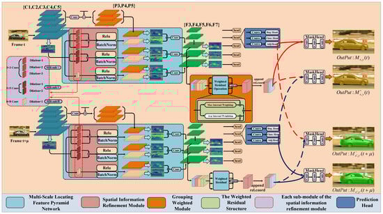
Figure 1.
The overall working pipeline of MLGW-VIS.
The dynamic instance mask generation process obtained by cross-learning the t frame and the frame can be expressed as follows:
In the above equations, represents the mask dynamic convolution, which takes the mask feature as input to generate the prediction mask after it is located in the mask branch. As shown in Figure 1, the output features of FPN F3, F4, F5, P6, and P7 are used as the input of shared heads such as classification head, regression head, center position head, and adjustment head. The dynamic convolution structure of the mask is changed by adjusting the parameters of the head so that different convolution layers are generated with the change in parameters. The mask dynamic convolution is used to generate appropriate mask structures for different frames of each video, and the mask features are input into the mask dynamic convolution to generate the prediction mask. Compared with the fixed mask convolution layer, the segmentation accuracy is greatly improved.
2.1. Spatial Information Refinement Module
Fisher Yu et al. [37] proposed dilated convolution, which makes the convolution layer keep the size of the feature map unchanged while increasing the receptive field. In this paper, a Spatial Information Refinement Module (SIR) is proposed where multi-level dilated convolution is used to extract feature maps from different degrees of receptive fields. The receptive field in the extracted features increases for multi-scale semantic information, and this information from low-level feature extraction of implementation is used to refine spatial information, while the features of the high-level feature space are employed to compensate for lack of location information. The SIR structure is as shown in Figure 1, which consists of three parts: spatial information refinement submodule I (SIR-SubI), submodule II (SIR-SubII), and submodule III (SIR-SubII), corresponding to the three branches of the SIR Structure in Figure 1 from top to bottom. The input features are generated by these three submodules, respectively, to generate dilated convolution feature maps of different scales. Then, they are mapped to the specified high-level feature map to obtain the multi-scale semantic information feature map, so that the high-level features can obtain richer semantic information. The first submodule consists of three 3 × 3 convolutions with dilation coefficients 1, 2 and 3, respectively. The second submodule consists of two 5 × 5 convolutions with dilation coefficients 1 and 2, respectively. The third sub-module is composed of an 8 × 8 convolution, and its expansion coefficient is 1. After the output of the three sub-modules, the activation function ReLU and batch normalization are used, respectively, to accelerate the convergence speed of the network. Through these three spatial information refinement sub-modules, low-level features can enable high-level feature maps to obtain multi-scale semantic information and receptive fields, making up for the loss of semantic features caused by the reduction in feature map size caused by multiple convolutions.
2.2. Multi-Scale Locating Feature Pyramid Network
In FPN, in order to supplement the low-level features with more high-level semantic information, the high-level features inside the FPN are upsampled and added. Although the top–down feature fusion operation allows the low-level features to obtain rich high-level semantic information, the high-level features output by FPN still have the problem of missing spatial location information. In this paper, we propose a Multi-Scale Locating Feature Pyramid Network (MSL-FPN). SIR is used to supplement the multi-scale spatial location information of the high-level feature maps of FPN, so that the high-level features of FPN can be more detailed and the localization ability of the network is enhanced.
MSL-FPN uses low-level features of the backbone network to map spatial location information and multi-scale receptive fields into high-level features. Firstly, the backbone network input feature map is subjected to a 7 × 7 convolution and 3 × 3 Max pooling to obtain C1, which is passed through four convolution layers of the backbone network in turn to obtain the output features C2, C3, C4, C5. Then, the size of each feature channel is uniformly compressed from 256, 512, 1024, 2048 to 256 by a 1 × 1 convolution. Finally, the feature map of the first layer is upsampled by bilinear interpolation from top to bottom in turn and added to the feature map of the next layer to obtain P3, P4, P5. The SIR is used to map the high-level features P3, P4, P5 with C1 as the low-level features. The specific operation is to make C1 generate different scale dilated convolution feature maps through spatial information refinement sub-modules SIR-subI, SIR-subII, and SIR-subIII, respectively. After that, the result is added with P3, P4, P5, respectively, and operated through a 3 × 3 convolution, and finally the output F3, F4, F5 of MSL-FPN can be obtained. The specific network structure diagram is shown in Figure 1, MSL-FPN part. The expression of feature hole mapping in MSL-FPN is as follows:
where (·) represents the convolution operation with a 3 × 3 kernel, and , respectively, represent the feature graphs in MSL-FPN (F3, F4, F5) and (P3, P4, P5); (·) denotes the 6-i submodule of SIR; is the first feature map C1 generated by convolutional pooling in the input backbone network shown in Figure 1.
Figure 2 shows the feature map visualization results of Layer C, Layer P, Layer F, and Layer C in MSL-FPN after the spatial information refinement sub-module. It can be seen from the results that the feature extraction effect of Layer P is significantly enhanced after the feature mapping of Layer C, which verifies that MSL-FPN can extract more key semantic features from feature maps. Figure 3 is the heat map visual comparison of the output features of the original network FPN and MSL-FPN in F3, F4, F5, P6, P7. The color of the heat map varies from blue to red, indicating that the heat value is from low to high. The higher the aggregation degree of the high heat value area in the heat map in the target area, the higher the attention of the network to the target area. It can be clearly seen from Figure 3 that MSL-FPN has a higher degree of high thermal value aggregation in the target area than the original network FPN, and the degree of high thermal value aggregation in the target area increases with the depth of the feature map, indicating that MSL-FPN can extract the spatial location information of low-level features to supplement the high-level features so as to locate the target more accurately.
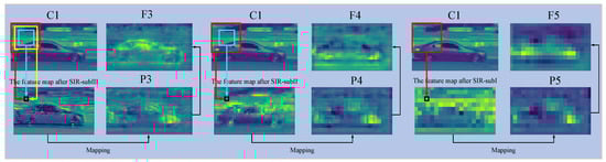
Figure 2.
The feature maps of MSL-FPN mapping effect.
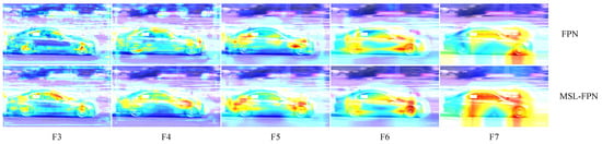
Figure 3.
Comparison of FPN and MSL-FPN heatmaps.
2.3. Grouping Weighted Module
The output features of MSL-FPN in Figure 1 are obtained after the mask branch convolutional layer. In order to reduce the number of parameters, the mask branch compacts the number of mask feature channels from 128 to 8. Moreover, the mask feature does not perform any cross-channel operation after passing through the convolutional layer of the mask branch, resulting in a lack of information interaction between the channels of the mask feature. To solve the above problems, we propose the Grouping Weighted Module (GWM), which is used after the mask branch convolutional layer to group the mask features, and perform cross-channel feature learning in the subspace of each group feature to solve the problem of weak interaction information and loss of deep semantic information in the masked feature dimension.
As shown in Figure 4, GWM average mask features according to the channel can be divided into four groups: , in which each group characteristics of the channel number is 2, and characteristics of each group are respectively sorted for empowerment residual operation. Firstly, the grouped features of each group are input into the grouped convolution of a single channel, and the feature information of each channel of the single group features is extracted, respectively. After that, it is input into the Max pooling layer and the average pooling layer to extract the salient semantic features and the mean semantic features, respectively. Then, the features extracted by the two pooling layers are subjected to 1 × 1 convolution for channel compression, and the number of channels is compressed from 2 to 1. After batch normalization and activation function, the results are input into the normalized exponential function to calculate their weights. Further, a 1 × 1 convolution is used to expand the number of channels to the pre-compression size. Finally, the calculated weights are multiplied with the original single set of features to obtain the maximum weighted feature and the average weighted feature, respectively, and then the two weighted features are added with the original single set of features to obtain the weighted residual feature. After the above operations, the four groups of features are concatenated according to the channel, and finally the group-weighted features that complete cross-channel learning in different subspaces are obtained. The mask feature of GWM makes up for the loss of deep semantic information caused by channel plunge. The GWM calculation process can be described as follows:
where denotes grouping weighted features; (·) represents the concatenation operation; , , , for the mask features divide the channel after each group; represents the internal pooling weighting operation for each group of features. is the Max pooling weighting in the internal pooling weighting operation. is the average pooling weighting in the internal pooling weighting operation. (·), (·), and (·) are max pooling, average pooling, and normalized exponential functions, respectively.
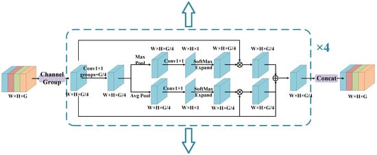
Figure 4.
Diagram of the GWM structure.
The mask features extracted by GWM are concatenated with the relative position matrix and then input into the mask dynamic convolution to make the semantic information of the mask features extracted by GWM more abundant so as to predict a more accurate instance mask.
2.4. Weakly Supervised Loss Construction
To conduct weakly supervision without mask annotation, two loss terms are introduced. Projection loss term is a loss function supervises the horizontal and vertical projections of the predicted mask using the ground-truth box annotation, which ensures that the tightest box covering the predicted mask matches the ground-truth box. Further, to obtain supervision within a bounding box, color similarity loss is introduced to supervise the mask in a pairwise way, which encourages predicted results for each pixel pair in an input image to be the same if the pair of pixels seem to have the same color.
2.4.1. Projection Loss
Projection loss [32] restricts the foreground and background probabilities of pixels in the image through the projection of the real bounding box so that the foreground prediction is distributed in the real bounding box as much as possible and the background prediction is distributed outside the real bounding box as much as possible.
The calculation process of projection loss is shown in Figure 5 where the left side is the true value of the bounding box. Assuming that the image pixel is a matrix of the form , the row matrix XG and the column matrix YG are established, respectively. The form is the and vector, respectively. The right side of Figure 5 is the prediction mask, and its image pixel matrix is in the form of . The maximum probability of the prediction mask pixel matrix being the foreground object is calculated in the row and column directions, respectively. The calculation result is value of the two vector matrices and . The two vector matrices are row matrix XM and column matrix YM, respectively; XM and YM are of the form and , respectively.
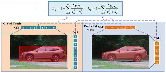
Figure 5.
Diagram of the projection loss.
Dice Loss is used to calculate projection loss, and the foreground probability distribution of image pixels is constrained to narrow the gap between XM, YM, XG, and YG so as to solve the problem of poor segmentation accuracy caused by the small proportion of small objects in the image. and are defined as orthogonal losses for row and column matrices, respectively, as follows:
Among them, and are XG and YG, respectively; represents the corresponding XM and YM; W and H are the width and height of the image.
The final projection loss can be obtained by adding the losses computed in the row and column directions:
2.4.2. Color Similarity Loss
Although projection loss is able to constrain the prediction mask to be within the true bounding box, further accurate segmentation of the pixel-wise instances inside the bounding box is hardly to be achieved. The color similarity loss [32] is introduced to obtain finer masks in the bounding box. The principle of color similarity loss is to calculate the color similarity between the pixel and its surrounding pixel and divide the pixel by a color similarity threshold. Then, the consistency classification of foreground or background is constrained by the pixel categories divided by color similarity in the image.
Color similarity loss is used to constrain the classification of the image foreground or background consistency so that the image pixels have the consistency of the foreground or background in the area of similar color and the instance targets in the bounding box are more accurately distinguished. As illustrated in Figure 6, first, an undirected graph is constructed on the image, where V is the sum of all the pixels in the image and E is the sum of all the edges in the image. The color similarity loss is calculated by combining the probability of foreground or background consistency predicted by pairs of pixels with the category of pixel determined by color similarity. During calculation, each pixel is connected with its surrounding 8 pixels. In order to increase the receptive field and make the calculation range of color similarity between pixels larger, the method of interval pixel sampling is used.
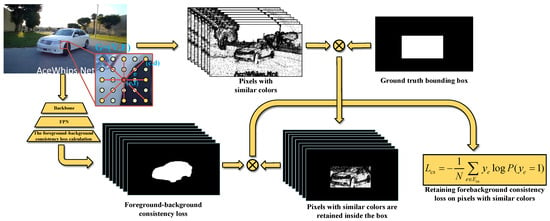
Figure 6.
Diagram of the color similarity loss.
Firstly, an edge is defined as e, and is the label of edge E. When , the two pixels connected by edge e have the same true value label, which means that the two pixels are both foreground or background. When , it means that two pixels have different labels, one for foreground and the other for background. Pixels (c, d) and (e, f) for the edge pixels are at the ends of the e, so network prediction can be seen as pixel (c, d) is the prospect of probability. The same can be said for (e, f) as the prospect of probability. Then, the probability calculation can be expressed as follows:
and the probability is calculated as follows:
Generally, the predicted probability distribution of the network can be trained with a binary cross-entropy loss, so the loss function can be expressed as
Among them, represents the set of edges that contain at least one pixel in the box. is used instead of the set of all edges E to avoid the loss calculation being affected by other irrelevant pixels outside the bounding box, which causes the color similarity loss to not properly constrain the prediction mask. N is the number of edges in inside the box. Loss function formula contains the color similarity , and is the sum of two cases of loss, but in practice, when is the label for unknown edges, it is easy to cause the network to distinguish the background of the target with error constraints. As a result, the accuracy of the prediction mask decreases, so the loss function in the case of is partially eliminated when using the color similarity loss, and the final color similarity loss function is obtained as follows:
3. Experimental Results and Analysis
3.1. Datasets
In this paper, common objects in street scenes are extracted on Youtube-VIS 2019 as the dataset of MLGW-VIS, in which the extracted dataset divides the instance objects into seven classes: train, truck, car, motorcycle, skateboard, human, and dog. The training set contains 329 video clips, the total number of video frames is 7212 frames, and a total of 603 instance targets are contained. The validation set contains 53 video clips, the total number of video frames is 1097 frames, and a total of 88 instance targets are contained. All the mask labels in the training set are removed and only the bounding box labels are retained for the training of the text weakly supervised network, and all the labels in the validation set are retained for the verification of the segmentation accuracy of the text weakly supervised network.
3.2. Evaluation Metrics
Average precision (AP) and average recall (AR) are used as the evaluation metrics in this paper. Average precision is the area under the PR curve, which is calculated by averaging the segmentation accuracy corresponding to the interval of Intersection over Union (IoU) threshold [0.50:0.05:0.95], and average recall is the percentage ratio of the objects correctly detected as positive samples to all instance objects in the video frame. Higher values of AP and AR indicate better segmentation effect, and the relevant calculation formula is as follows:
where is the number of objects correctly detected as positive, is the number of objects incorrectly detected as positive, and is the number of objects missed as positive. Compared with image instance segmentation, the IoU of video instance segmentation increases the calculation in the time domain. For example, given a video with F frames, by calculating the ratio of the intersection sum and the union sum of the predicted mask and the true mask of the same category in each frame, the IoU of a certain class of objects in the video can be obtained, and the MIoU can be obtained by calculating the average IoU of all classes. The formula for calculating IoU is as follows:
where f represents the total number of frames in the video, f represents the fth frame of the video, P and T refer to the predicted value and the true value of the instance, respectively, and m represents the instance of the current frame in the video.
3.3. Experimental Platform
The hardware for the experiments in this paper includes a CPU of Intel i5 10400F and a GPU of MSI GeForce RTX 3060 GAMING X TRIO 12G, software environment for Ubuntu18.04, CUDA 11.1, cuDNN—8.0.5, python 3.7, and deep learning framework Pytorch—1.8.
In this paper, the experiment is based on the Pytorch deep learning framework to perform building on the basis of the CrossVIS network. In the training process, the data loader is input into the network with a uniform size of 360 × 640. A total of 23,000 iterations are used for training, the number of loop iterations for the complete dataset is 12 epochs, the batch size is set to 4, and the initial learning rate is set to 0.005. The weight decay mode is linear.
3.4. Experimental Results
3.4.1. Multi-Scale Localization Feature Pyramid Experiment Analysis
In the CrossVis-based Weakly supervised benchmark network (CWVIS), the high-level features of FPN have the problems of lack of spatial location information and lack of semantic information caused by single receptive field. In order to solve these problems, this paper proposes MSL-FPN. The spatial information refinement of FPN output features is realized so as to enhance the correlation between FPN output features and low-level feature sets. As shown in Table 1, in this paper, we perform three ablation experiments on MSL-FPN and compare them with CWVIS, where sub1, sub2, and sub3 denote SIR-subI, SIR-subII, and SIR-subIII, respectively. The segmentation accuracy of CWVIS is 32.2%. On the basis of CWVIS, the average segmentation accuracy of SIR-subIII, SIR-subII, and SIR-subI on FPN features P3, P4, P5 is 34.3%, 35.8%, and 36.6%, respectively. Compared with the segmentation results using SIR only, it improves by 2.1%, 3.6%, and 4.4%, respectively. The experimental results show that the network complements the spatial position information and receptive field of high-level features by MSL-FPN, which effectively improves the average segmentation accuracy of the network.

Table 1.
Comparison of the results of multi-scale localization feature pyramid experiments of different structures.
3.4.2. Experimental Analysis of Group Weighting Module
In order to verify the influence of the number of GWM groups on the network segmentation accuracy, this section conducts experiments on multiple different grouping situations of GWM based on the addition of MSL-FPN to obtain the number of groups when it improves the network segmentation accuracy best. First of all, we set the number of groups as 1, 2, 4, and 8, and they are denoted as G1, G2 and G3, G4. The experimental results are shown in Table 2, under the same experimental conditions for GWM to experiment with different structures. The average segmentation accuracy of GWM with the number of groups of 1, 2, 4 and 8 is 35.3%, 36.6%, 37.9%, and 36.6%, respectively, which is 3.1%, 4.4%, 5.7%, and 4.4% higher than that of CWVIS. It can be seen from Table 2 that the network segmentation effect is the best when the number of groups is set to 4, indicating that GWM has the best effect on the depth semantic information supplement of mask features and channel interaction in the subspace under this configuration.
Table 2.
Comparison of the influence of the number of block weights on the segmentation accuracy.
3.4.3. Ablation Experiments of MLGW-VIS
In this paper, the CrossVIS network is modified into a weakly supervised video instance segmentation network, and MSL-FPN and GWM are proposed to improve the problems existing in the network. This section conducts ablation experiments on the two modules on the basis of CWVIS to verify its effectiveness on the network. The experimental results are shown in Table 3. When MSL-FPN is used on the basis of CWVIS alone, the segmentation accuracy is 36.6%, which is 4.4% higher than that of the baseline CWVIS. When GWM is added only at the mask branch, the average segmentation accuracy of the network reaches 36.2%, which is 4% higher than that of the baseline CWVIS. The combination of the above two modules in CWVIS achieves the best segmentation accuracy of 37.9%, which is 5.7% higher than that of the baseline CWVIS. According to the experimental results in Table 1, the segmentation accuracy of MSL-FPN and GWM separately added to CWVIS is significantly improved, and when the two modules are used in the network at the same time, the average segmentation accuracy is better than the performance of the two modules alone, which verifies the effectiveness of the proposed MLGW-VIS algorithm.
Table 3.
The ablation results of this method are obtained.
3.4.4. Comparison with the Experimental Results of Different Networks
Considering that there are few weakly supervised video instance segmentation networks at present, this paper chooses the fully supervised networks CrossVIS, YolactEdge, and ST-Mask to compare with MLGW-VIS, respectively, and the experiments are carried out under the same equipment and environment. The experimental results of each network in Table 4 show that the average accuracy of MLGW-VIS reaches 37.9%, which is 3% higher than that of the fully supervised network YolactEdge, but the segmentation speed is reduced by 9.8FPS, which is 5.7% higher than that of the benchmark weakly supervised network CWVIS. Compared with the fully supervised network, the average accuracy of STMask and CrossVIS is only 2.1% and 2.7%respectively. MLGW-VIS significantly reduces the cost of dataset labeling compared with the fully supervised network and can achieve real-time segmentation speed of 34.6FPS on a graphics card 2080Ti. The experimental results show that the segmentation accuracy of the weakly supervised video instance segmentation method is comparable to that of some current mainstream fully supervised networks, which further proves the effectiveness and feasibility of the MLGW-VIS network. The visual output results of CWVIS and our method are provided in Figure 7, where we can see the significant improvement of our designs.
Table 4.
Comparison of experimental results of different networks.
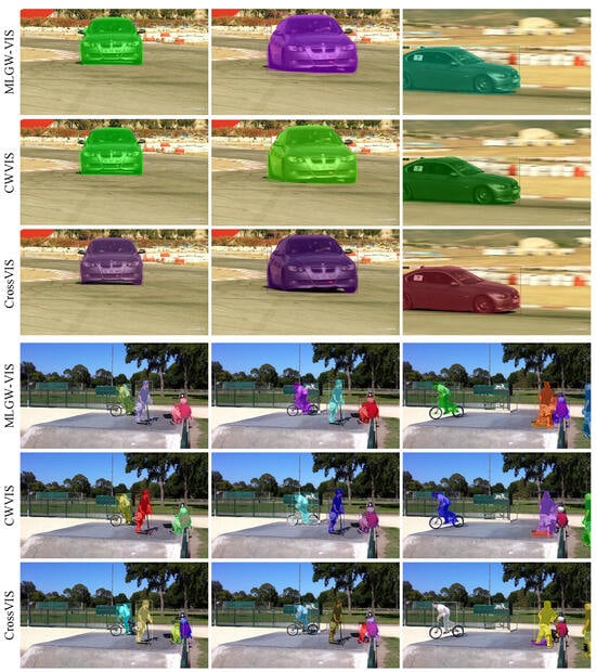
Figure 7.
Segmentation result visualization.
4. Model Application on Air Cruiser
In this paper, a weakly supervised video instance segmentation network MLGW-VIS is established to alleviate the modeling inefficiency caused by the complex sample labeling of the fully supervised algorithm and improve the accuracy of the model. In addition to efficient modeling for fast mission response, vision-based target localization is a key factor for accurate and effective air mission. In the rapidly changing mission environment, the space position of a large number of ground targets changes continuously with time. The air cruiser equipped with a vision device and a video instance segmentation model can better sense the environment and obtain task-related information on the basis of real-time perception from its own position coordinate. It is helpful to quickly perceive the situation of the task scene and the position of the target instance so as to further realize autonomous cruise obstacle avoidance.
In this chapter, the air cruiser platform and flight control base station are built, and the software system with function modules of video sample collection, object instance segmentation visualization, and location coordinate solution is developed. The video instance segmentation model designed in this paper is put into use by the Open Neural Network Exchange (ONNX) format for weight deployment of lossless migration across programming platforms, and the video target pixel area identification and GPS coordinate positioning of the cruiser are realized. The feasibility of the system and the positive effect of the research content on improving the accuracy of target positioning are verified by experiments.
4.1. Flight System
The air cruiser is assembled based on an F450 quad-rotor frame, and four 20A electric and four 2212 KV950 servo motors are used to drive the 4-axis rotor. The four motors of the air cruiser are servo controlled through the Pixhawk 2.4.8 open source flight control embedded program. At the same time, the signal transceiver device is combined with the base station and controller for remote communication. Pixhawk flight control uses a 32-bit STM32F427 chip with FPU using a Cortex M4 core; the main frequency is 168 MHz with a 252MIPS computing power, 256 KB RAM, and a 2 MB flash memory, and a fault co processor chip with a model of STM32F103. In addition, the cruiser uses the NEO series high-precision positioning module produced by the Swiss u-blox combined with the M8N GPS module to carry out the geographical coordinates, and the limit accuracy is about 0.5 m. In this paper, FS-I6 remote controller is used for ground control in frequency band of 2.4 GHz.
The overall flight control architecture is shown in Figure 8. The controller controls the device by mode switching and flight control commands issued by rocker operation through the remote control connected with the base station calibration. The communication between the remote control and the signal receiver is through the 2.4 GHz frequency band, and the signal receiver is connected with the flight control hardware through the Pin interface. Furthermore, the remote signal is converted into the motor servo signal to complete the control of the four-axis motor. The flight control base station is developed and deployed on the laptop. The laptop and the airborne end are connected by wireless data transmission to establish MAVLink protocol communication between the flight control base station and the air cruiser device so as to obtain real-time feedback of various parameters and transmission of base station control signals.
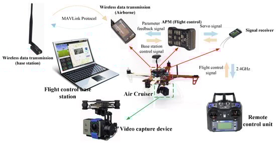
Figure 8.
The platform structure diagram of the air cruiser control system.
4.2. Instance Segmentation and Localization
Our network is built by Python for code programming and model training output in Linux system. In order to use the model to carry out image sample inference in the cross-platform Winform software with better performance, ONNX conversion and C# ONNX Runtime invocation of the trained video instance segmentation model.pt weight file are required. Firstly, the Onnxruntime environment code is introduced into Python and the onnx.export function is called to sort out the weight value of the model, the network flow information of the neural network, the input and output information of each layer network, and other auxiliary information and output it into an ONNX file. Then, the converted video instance segmentation model ONNX file is imported into the flight control software running directory, and the InferenceSession object is created by the API of ONNX Runtime in C# project to load the model in ONNX format. Subsequently, input data are prepared according to the requirements of the model, which involves image preprocessing (such as scaling, normalization, etc.), and the preprocessed input data are passed to the model, and the output of the model is obtained. Then, the ONNX model is calculated to obtain the float DenseTensor including mask features, mask predictions, and bounding box regression predictions to perform three tasks of classification, bounding box regression localization, and instance mask region color coverage, respectively. In addition, the Rectangle function of OpenCVSharp is introduced to build the rectangular boxes of instances according to the bounding box regression corners. The PutText function is applied to label and draw the scores of the instances and probabilities and construct the rectangular boxes for the instances. Next, the mask areas are generated after the mask feature binarization process and the output is shown in Figure 9. Finally, the instance positioning coordinates are solved based on the instance mask center point coordinates.
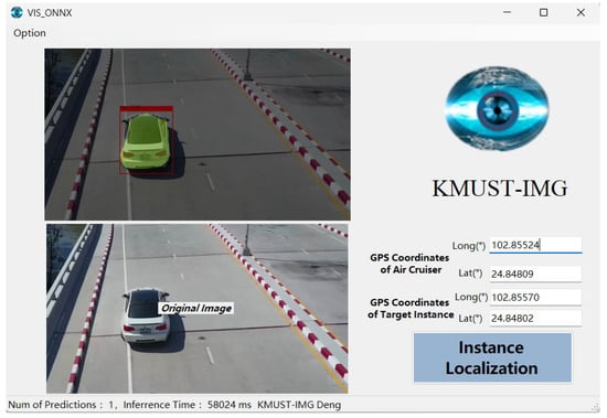
Figure 9.
Diagram of video instance segmentation and positioning output.
The location of target instance is mainly solved by the geometric relationship model between image point and target point. The ideal projection imaging model is the central projection in optics, which refers to the camera model in which all objects are projected onto the imaging plane through the center point of the camera optical axis. In this chapter, the ideal plane camera model is used to approximate the actual vision acquisition device. As shown in Figure 10, the photosensitive element of the visual acquisition device of the navigator is first established as the coordinate point C, and the axis w is the lens optical axis. Then, the origins of the world coordinate system W and the corresponding coordinate system are established, in which the world coordinates of the origin of the photosensitive element are . According to the principle of similar triangle, the parameter relationship can be obtained as follows:
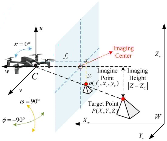
Figure 10.
Target localization geometric relationship diagram.
Further, according to the image coordinates of the image point o with the camera focal length transformation, the world coordinates of the cruise flying origin are C and the target world coordinates are in and directions from , . Further, we consider the Earth as a regular sphere, where the Earth’s radius is 6,371,000 m, the circumference of any Earth’s longitude is 40030173, and the circumference of a particular latitude can be calculated as meters. On the basis of combining cruise flying shot coordinates calculating the target coordinates, the specific expression is
4.3. Experiments
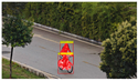
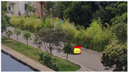
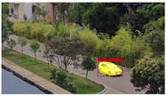
Since the video transmission rate and the inference speed of flight control base station are not capable of real-time operation, the experiment in this chapter is aimed at collecting image samples from the air cruiser view, segment offline instances, and solve coordinates. First of all, the experiment collects video samples from the view angle of the cruiser at a height of 10 m from the ground and then records coordinates of the target position of the video example with reference to the handheld GPS positioning instrument. The shooting horizontal angle is −90°, the tilt angle is maintained at 0°, and the vertical right angle is set at 90°; that is, the shooting is always perpendicular to the ground and facing the west using a focal length of f = 70 mm and the frame rate is 30fps. In the interface, Long is the coordinate longitude value and Lat is the latitude value. Among them, the GPS coordinates where the cruiser’s viewing angle is taken are (102°51′18.864″, 24°50′53.124″). The sample of cyclists located at GPS coordinates (102°51′17.031″, 24°50′53.840″) is set to carry out the experiment, and the distance of the sample from the ground shooting coordinates is about 60 m. The ONNX conversion of CWVIS and the innovative model MLGW-VIS proposed in this study is carried out and deployed in the flight control software. Video instance segmentation and GPS coordinate positioning are performed on all instances in the sample, and the real GPS coordinate values are recorded by the handheld positioning instrument. The segmentation visualization results are shown in Table 5. It can be seen that the innovative model MLGW-VIS proposed in this study has obvious advantages in the segmentation effect. Especially when the target instance is far away and the target image is small, the segmentation is more complete and the edge is more detailed, and the instance identification of the bicycle and the human body is accurate. The experimental results of the GPS coordinate solution are shown in Table 5. It can be seen that there is a larger coordinate error between the weakly supervised baseline model and the coordinates of reference personnel in the GPS solution results, while our MLGW-VIS proposed in this paper provides a better mask area after optimization, thus making the example positioning results more accurate.
Table 5.
Target instance ONNX model deployment segmentation and localization results.
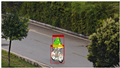
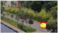
In addition, we perform segmentation visualization and target positioning on a continuous motion video data of the car instance and demonstrate our positioning effect by indexing GPS coordinates in a real electronic map. The relevant experimental results of the ONNX model using MLGW-VIS are presented in this paper as shown in Table 6. From the segmentation visualization results, it can be seen that our model still obtains excellent mask prediction quality when the instance is obscured, and it is finely segmented during continuous motion.
Table 6.
Target instance ONNX model deployment segmentation visualization and the corresponding map mark.
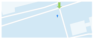
According to the GPS coordinates obtained by inference, we index and mark the anchor points from the electronic map with the blue mark showing the positioning results obtained by the program in this chapter and the green arrow mark showing the location on the actual road. It can be seen that the positioning results obtained in this chapter basically maintain the same map error as the actual road position, and the motion trajectory is basically consistent. Considering the width of the actual road and the position deviation of the car, the localization results shows high accuracy and application value of the for air cruiser.
In our research, experimental results show that MLGW-VIS can achieve real-time inference (34.6 FPS) in Python, Linux system using 2080Ti. However, the ONNX model deployment can only reserve model accuracy while the inference speed is highly deepened on the C# program and resource optimization. In the revised manuscript, the inference speed of our method on the embedded system is provided. Although the speed is decreased to nearly 8 FPS (latency 144 ms), it still provides a full example of VIS model training to deployment with acceptable performance for common lowspeed target on the ground. Meanwhile, only a maximum 4 GB graphic memory is required, which is easily obtained in common application.
5. Results
Abundant experimental results are obtained in our work. For the designs with MSL-FPN used on the basis of CWVIS alone, the segmentation accuracy is 36.6%, which is 4.4% higher than that of the baseline CWVIS. When GWM is added only at the mask branch, the average segmentation accuracy of the network reaches 36.2%, which is 4% higher than that of the baseline CWVIS. The combination of the above two modules in CWVIS achieves the best segmentation accuracy of 37.9%, which is 5.7% higher than that of the baseline CWVIS. The experimental results show that MLGW-VIS is on par with mainstream fully supervised CNN-based networks in terms of segmentation accuracy and speed. Experiments on the air cruiser also show that the research has positive effects on improving the perception and localization accuracy in air cruiser application. The results prove that our method can effectively use the space location and depth of the semantic information to improve the network of target segmentation accuracy.
6. Conclusions
In this paper, we propose a weakly supervised video instance segmentation network MLGW-VIS that complements multi-scale deep semantic information to achieve accurate object localization and segmentation without mask labeling. Firstly, aiming at the problem of rough spatial information of high-level features and weak correlation with low-level features of FPN, MSL-FPN is proposed. SIR is used to extract rich spatial location information and multi-scale receptive field of low-level features, and it is added to high-level features to make up for the missing part of spatial location information. The correlation between the output features of FPN and the low-level feature set is enhanced. Secondly, GWM is added after the mask branch, and the mask features are divided into four groups and the weighted residual operation is performed on the features of each group so that each group of feature subspaces is separately mapped to supplement the depth semantic information and enhance the information interaction between channels in the subspace. Further, the mask loss part is modified by the projection loss and the color similarity loss so that the network can supervise the prediction mask only using the bounding box annotation and the semantic information of the image itself. Finally, an air cruiser platform is built to deploy the trained MLGW-VIS model for segmentation and localization of target instances. The experimental results show that MLGW-VIS is on par with mainstream fully supervised CNN-based networks in terms of segmentation accuracy and speed and has positive effects on improving the perception and localization accuracy in air cruiser application.
7. Discussion
Although the proposed MLGW-VIS has made progress, there are still limitations. The rough bounding box annotations reduce the quality of the segmentation mask, and even with the assistance of projection and color similarity loss, MLGW-VIS still fails to completely replace the segmentation effect of the fully supervised network. Additionally, our method unilaterally improves the frame-level instance segmentation accuracy, ignoring the effectiveness of the temporal information in the tracking task of instances. Therefore, our future weakly supervised video instance segmentation research will focus on introducing optical flow and other techniques to improve temporal features and attempt to reduce the model size to achieve real-time functions on the air cruiser.
8. Future Work
Based on the limitations of our research, our future weakly supervised video instance segmentation work will focus on introducing optical flow and other techniques to improve temporal features and attempt to reduce the model size to achieve real-time functions on the air cruiser.
Author Contributions
Conceptualization, Y.D.; methodology, Y.D.; software, Y.D.; validation, Y.L.; formal analysis, Y.L.; investigation, Y.L and Z.H.; resources, Y.Z.; data curation, Y.D.; writing—original draft preparation, Y.D.; writing—review and editing, Y.D., Y.L., Y.Z. and Z.H.; visualization, Y.D.; supervision, Z.H.; project administration, Y.Z. and Z.H.; funding acquisition, Y.Z. and Z.H. All authors have read and agreed to the published version of the manuscript.
Funding
This work was supported by the National Natural Science Foundation of China under Grants 62061022 and 62171206, The Open Fund Project of the Key Laboratory of Intelligent Application of Equipment of the Ministry of Education for ground time-sensitive target location technology based on multi-cruiser cooperative detection.
Data Availability Statement
The data YouTube-VIS used in this paper can be publicly downloaded and the results verified on the website https://youtube-vos.org/, (accessed on 25 February 2025). The images from the UAV perspective are currently not available for public use since this research is limited by the privacy policy of the funder.
Conflicts of Interest
The authors declare that they have no known competing financial interests or personal relationships that could have appeared to influence the work reported in this paper.
References
- Liu, X.; Liu, W.; Wu, A. Design of a Lung Lesion Target Detection Algorithm Based on a Domain-Adaptive Neural Network Model. Appl. Sci. 2025, 15, 2625. [Google Scholar] [CrossRef]
- Zhu, S.; Wang, Y. Multi-level similarity transfer and adaptive fusion data augmentation for few-shot object detection. J. Vis. Commun. Image Represent. 2024, 105, 104340. [Google Scholar] [CrossRef]
- Duan, S.; Wang, T.; Li, T.; Yang, W. M-YOLOv8s: An improved small target detection algorithm for UAV aerial photography. J. Vis. Commun. Image Represent. 2024, 104, 104289. [Google Scholar] [CrossRef]
- Hwang, D.; Kim, J.J.; Moon, S.; Wang, S. Image Augmentation Approaches for Building Dimension Estimation in Street View Images Using Object Detection and Instance Segmentation Based on Deep Learning. Appl. Sci. 2025, 15, 2525. [Google Scholar] [CrossRef]
- Fedon Vocaturo, M.; Altabella, L.; Cardano, G.; Montemezzi, S.; Cavedon, C. Unsupervised Learning Techniques for Breast Lesion Segmentation on MRI Images: Are We Ready for Automation? Appl. Sci. 2025, 15, 2401. [Google Scholar] [CrossRef]
- Bai, S.; Liang, C.; Wang, Z.; Pan, W. Information entropy induced graph convolutional network for semantic segmentation. J. Vis. Commun. Image Represent. 2024, 103, 104217. [Google Scholar] [CrossRef]
- Jin, Z.; Dou, F.; Feng, Z.; Zhang, C. BSNet: A bilateral real-time semantic segmentation network based on multi-scale receptive fields. J. Vis. Commun. Image Represent. 2024, 102, 104188. [Google Scholar] [CrossRef]
- Bayraktar, E. ReTrackVLM: Transformer-Enhanced Multi-Object Tracking with Cross-Modal Embeddings and Zero-Shot Re-Identification Integration. Appl. Sci. 2025, 15, 1907. [Google Scholar] [CrossRef]
- Cheng, X.; Zhao, H.; Deng, Y.; Shen, S. Multi-Object Tracking with Predictive Information Fusion and Adaptive Measurement Noise. Appl. Sci. 2025, 15, 736. [Google Scholar] [CrossRef]
- Wei, L.; Zhu, R.; Hu, Z.; Xi, Z. UAT:Unsupervised object tracking based on graph attention information embedding. J. Vis. Commun. Image Represent. 2024, 104, 104283. [Google Scholar] [CrossRef]
- He, K.; Gkioxari, G.; Dollár, P.; Girshick, R. Mask R-CNN. In Proceedings of the 2017 IEEE International Conference on Computer Vision (ICCV), Venice, Italy, 22–29 October 2017; pp. 2980–2988. [Google Scholar] [CrossRef]
- Feng, Q.; Yang, Z.; Li, P.; Wei, Y.; Yang, Y. Dual Embedding Learning for Video Instance Segmentation. In Proceedings of the 2019 IEEE/CVF International Conference on Computer Vision Workshop (ICCVW), Seoul, Republic of Korea, 27–28 October 2019; pp. 717–720. [Google Scholar] [CrossRef]
- Wang, Q.; He, Y.; Yang, X.; Yang, Z.; Torr, P. An Empirical Study of Detection-Based Video Instance Segmentation. In Proceedings of the 2019 IEEE/CVF International Conference on Computer Vision Workshop (ICCVW), Seoul, Republic of Korea, 27–28 October 2019; pp. 713–716. [Google Scholar] [CrossRef]
- Liu, X.; Ren, H.; Ye, T. Spatio-Temporal Attention Network for Video Instance Segmentation. In Proceedings of the 2019 IEEE/CVF International Conference on Computer Vision Workshop (ICCVW), Seoul, Republic of Korea, 27–28 October 2019; Volume 10, pp. 725–727. [Google Scholar] [CrossRef]
- Dong, M.; Wang, J.; Huang, Y.; Yu, D.; Su, K.; Zhou, K.; Shao, J.; Wen, S.; Wang, C. Temporal Feature Augmented Network for Video Instance Segmentation. In Proceedings of the 2019 IEEE/CVF International Conference on Computer Vision Workshop (ICCVW), Seoul, Republic of Korea, 27–28 October 2019; Volume 10, pp. 721–724. [Google Scholar] [CrossRef]
- Cao, J.; Anwer, R.M.; Cholakkal, H.; Khan, F.S.; Pang, Y.; Shao, L. SipMask: Spatial Information Preservation for Fast Image and Video Instance Segmentation. In Proceedings of the ECCV, Glasgow, UK, 23–28 August 2020. [Google Scholar]
- Fu, Y.; Yang, L.; Liu, D.; Huang, T.S.; Shi, H. CompFeat: Comprehensive Feature Aggregation for Video Instance Segmentation. arXiv 2020, arXiv:2012.03400. [Google Scholar]
- Lin, C.C.; Hung, Y.; Feris, R.; He, L. Video Instance Segmentation Tracking With a Modified VAE Architecture. In Proceedings of the 2020 IEEE/CVF Conference on Computer Vision and Pattern Recognition (CVPR), Seattle, WA, USA, 13–19 June 2020; pp. 13144–13154. [Google Scholar] [CrossRef]
- Liu, D.; Cui, Y.; Tan, W.; Chen, Y. SG-Net: Spatial Granularity Network for One-Stage Video Instance Segmentation. arXiv 2021, arXiv:2103.10284. [Google Scholar]
- Liu, H.; Rivera Soto, R.A.; Xiao, F.; Lee, Y.J. YolactEdge: Real-time Instance Segmentation on the Edge. In Proceedings of the 2021 IEEE International Conference on Robotics and Automation (ICRA), Xi’an, China, 30 May–5 June 2021; pp. 9579–9585. [Google Scholar] [CrossRef]
- Carion, N.; Massa, F.; Synnaeve, G.; Usunier, N.; Kirillov, A.; Zagoruyko, S. End-to-End Object Detection with Transformers. In Proceedings of the ECCV, Glasgow, UK, 23–28 August 2020. [Google Scholar]
- Wang, Y.; Xu, Z.; Wang, X.; Shen, C.; Cheng, B.; Shen, H.; Xia, H. End-to-End Video Instance Segmentation with Transformers. In Proceedings of the 2021 IEEE/CVF Conference on Computer Vision and Pattern Recognition (CVPR), Nashville, TN, USA, 20–25 June 2021. [Google Scholar]
- Wu, J.; Jiang, Y.; Bai, S.; Zhang, W.; Bai, X. SeqFormer: Sequential Transformer for Video Instance Segmentation. In Proceedings of the ECCV, Tel Aviv, Israel, 23–27 October 2022. [Google Scholar]
- Cheng, B.; Misra, I.; Schwing, A.G.; Kirillov, A.; Girdhar, R. Masked-attention Mask Transformer for Universal Image Segmentation. In Proceedings of the 2022 IEEE/CVF Conference on Computer Vision and Pattern Recognition (CVPR), New Orleans, LA, USA, 18–24 June 2022; pp. 1280–1289. [Google Scholar] [CrossRef]
- Vaswani, A.; Shazeer, N.; Parmar, N.; Uszkoreit, J.; Jones, L.; Gomez, A.N.; Kaiser, L.; Polosukhin, I. Attention is All You Need. In Proceedings of the NeurIPS, Long Beach, CA, USA, 4–9 December 2017. [Google Scholar]
- Yang, S.; Fang, Y.; Wang, X.; Li, Y.; Fang, C.; Shan, Y.; Feng, B.; Liu, W. Crossover Learning for Fast Online Video Instance Segmentation. In Proceedings of the 2021 IEEE/CVF International Conference on Computer Vision (ICCV), Montreal, QC, Canada, 10–17 October 2021; pp. 8023–8032. [Google Scholar] [CrossRef]
- Tian, Z.; Shen, C.; Chen, H. Conditional Convolutions for Instance Segmentation. In Proceedings of the ECCV, Glasgow, UK, 23–28 August 2020. [Google Scholar]
- Zhou, B.; Khosla, A.; Lapedriza, A.; Oliva, A.; Torralba, A. Learning Deep Features for Discriminative Localization. In Proceedings of the 2016 IEEE Conference on Computer Vision and Pattern Recognition (CVPR), Las Vegas, NV, USA, 27–30 June 2016; pp. 2921–2929. [Google Scholar] [CrossRef]
- Ahn, J.; Cho, S.; Kwak, S. Weakly supervised learning of instance segmentation with inter-pixel relations. In Proceedings of the 2019 IEEE/CVF Conference on Computer Vision and Pattern Recognition (CVPR), Long Beach, CA, USA, 15–20 June 2019. [Google Scholar]
- Liu, Q.; Ramanathan, V.; Mahajan, D.; Yuille, A.; Yang, Z. Weakly Supervised Instance Segmentation for Videos with Temporal Mask Consistency. In Proceedings of the 2021 IEEE/CVF Conference on Computer Vision and Pattern Recognition (CVPR), Nashville, TN, USA, 20–25 June 2021; pp. 13963–13973. [Google Scholar] [CrossRef]
- Yan, L.; Wang, Q.; Ma, S.; Wang, J.; Yu, C. Solve the Puzzle of Instance Segmentation in Videos: A Weakly Supervised Framework With Spatio-Temporal Collaboration. IEEE Trans. Circuits Syst. Video Technol. 2023, 33, 393–406. [Google Scholar] [CrossRef]
- Tian, Z.; Shen, C.; Wang, X.; Chen, H. BoxInst: High-Performance Instance Segmentation With Box Annotations. In Proceedings of the 2021 IEEE/CVF Conference on Computer Vision and Pattern Recognition (CVPR), Nashville, TN, USA, 20–25 June 2021; pp. 5443–5452. [Google Scholar]
- Wang, X.; Feng, J.; Hu, B.; Ding, Q.; Ran, L.; Chen, X.; Liu, W. Weakly-supervised Instance Segmentation via Class-agnostic Learning with Salient Images. In Proceedings of the CVPR, Nashville, TN, USA, 20–25 June 2021. [Google Scholar]
- Zhou, Y.; Zhu, Y.; Ye, Q.; Qiu, Q.; Jiao, J. Weakly Supervised Instance Segmentation Using Class Peak Response. In Proceedings of the 2018 IEEE/CVF Conference on Computer Vision and Pattern Recognition, Salt Lake City, UT, USA, 18–23 June 2018; pp. 3791–3800. [Google Scholar] [CrossRef]
- Hsu, C.C.; Hsu, K.J.; Tsai, C.C.; Lin, Y.Y.; Chuang, Y.Y. Weakly supervised instance segmentation using the bounding box tightness prior. In Proceedings of the NeurIPS, Vancouver, BC, Canada, 8–14 December 2019. [Google Scholar]
- He, K.; Zhang, X.; Ren, S.; Sun, J. Deep Residual Learning for Image Recognition. In Proceedings of the 2016 IEEE Conference on Computer Vision and Pattern Recognition (CVPR), Las Vegas, NV, USA, 27–30 June 2016; pp. 770–778. [Google Scholar] [CrossRef]
- Yu, F.; Koltun, V. Multi-Scale Context Aggregation by Dilated Convolutions. arXiv 2016, arXiv:1511.07122. [Google Scholar]


Disclaimer/Publisher’s Note: The statements, opinions and data contained in all publications are solely those of the individual author(s) and contributor(s) and not of MDPI and/or the editor(s). MDPI and/or the editor(s) disclaim responsibility for any injury to people or property resulting from any ideas, methods, instructions or products referred to in the content. |
© 2025 by the authors. Licensee MDPI, Basel, Switzerland. This article is an open access article distributed under the terms and conditions of the Creative Commons Attribution (CC BY) license (https://creativecommons.org/licenses/by/4.0/).