Qutrit Control for Bucket Brigade RAM Using Transmon Systems

Abstract

Qudits allow the encoding and manipulation of additional quantum information compared to that stored to a two-level qubit system. Although manipulations of qudit states are generally more complex and can introduce extra sources of noise, qudits can still be used in a number of applications when this error can be kept sufficiently low. One such application is the case of the Bucket Brigade Algorithm for realizing a Quantum RAM (QRAM), which inherently uses qutrits for encoding the state of address switches. In this paper, we study a methodology for qutrit manipulation that leverages efficient encoding techniques and pulse calibration methods for the case of transmon systems. The methodology employs an encoding scheme that allows the execution of controlled operations, using the subspace spanned by the two lowest levels of the transmon; we show how this scheme can be used for generating one- and two-qutrit gates by leveraging the Qiskit and Boulder Opal frameworks to compute the parameters of pulses that implement the quantum gates that are used by the BBA. For this type of gate, simulations show that the pulses perform the required operations with a low infidelity when errors introduced by the qutrit Hamiltonian dynamics are considered.

1. Introduction

Although qubits logically represent two-level quantum systems, physical implementations are typically realized by systems that possess extra physical states. Good candidate architectures for implementing qubits are those that can efficiently isolate a two-level subsystem so that information does not leak to other states; fluxonium [1] and transmon [2] qubits are typical examples of such architectures. However, these extra states can be manipulated in many cases either to facilitate the computation in the two-level scheme or to expand the computational schema to include additional logical states. Tsukanov [3], for example, has demonstrated efficient pulses for single-qubit operations in a double donor structure; the pulses make use of the excited delocalized orbitals for achieving state transfer between the localized states used for encoding the logical qubit.

Going beyond the two-level logical qubit, the concept of qudit is used to denote any quantum information system that contains an n-level logical state. Examples of these systems are qutrit (three-level system), ququart (four-level system), and so on. Similarly to qubit operations, it can be demonstrated that universal gate sets for qudits can also be derived. As shown by Brylinski and Brylinski [4], any two-qudit gate V, combined with the collection of all 1-qudit gates A, constitutes a universal gate set, provided that V is imprimitive. An imprimitive 2-qudit gate is one that when acting on a decomposable state, its output is a state that, in general, cannot be decomposed. For example, if two qudits with states ${|x\rangle }_0$ and ${|x\rangle }_1$ are acted upon by the operator V, then the resulting state $V\left({|x\rangle }_0{|x\rangle }_1\right)$ cannot be decomposed into a product of the form ${|y\rangle }_0{|y\rangle }_1$, with ${|y\rangle }_i$ being single-qudit states. This situation is similar and can, in fact, be considered a generalization to universality requirements for qubit gates, where at least one entangling gate is required for a gate set to be universal. Wang et al. [5] also studied and demonstrated the existence of universal gate sets for qudits, while also reviewing the extent to which alternative quantum computational models based on qubits, such as measurement-based computing, adiabatic quantum computing, and topological quantum computing, can also be adopted for qudit-based computation. One particularly interesting use case is the possibility of using hybrid qudit computation, in which qudits of different dimensions are used; such hybrid approaches may offer more efficient algorithms when the problem to be solved has some natural mappings that are better served by nonbinary mappings (e.g., simulation of massive spin 1 systems). An algorithm for factorization using a hybrid approach has already been presented in [6], where one spin $3/2$ nuclei coupled with a spin 1 nuclei was used to encode qudits of dimensions four and three, respectively.

One particular domain of the application of qudits that is also relevant to the scope of the present work is its usage to compress quantum information in a manner that minimizes the amount of operations and/or qubits needed to perform calculations. In this direction, Baker et al. [7] have shown that by using qudits, it is possible to completely remove ancilla qubits when their number is $O\left(n\right)$ and produce an equivalent quantum circuit based on qudits with the same order of depth. On the other hand, Gokhale et al. [8] constructed a logarithmic depth decomposition scheme of the Toffoli gate based on qutrits, which uses no ancilla qubits or qutrits. Two of the authors of the present work have moreover shown that by using higher-energy states, quantum entanglement can be performed at the logical level by only using the spectrum of a single transmon [9].

Since each quantum hardware can support natively different types of pulses and two-qudit entanglement, the choice of single-qudit and two-qudit gates will naturally be different for each architecture. For the regime of the transmon-based architecture, for example, Fisher et al. [10] have shown that qudit control can be efficiently implemented and have obtained excellent experimental results for the case of a cross-resonance gate in a two-ququart system. On the other hand, Chi et al. [11] demonstrated an implementation scheme of a qudit processor that uses silicon-photonic integrated circuits.

One of the main challenges of quantum computation is the design of efficient quantum circuits and finding optimal transpilations for decomposing the logical quantum circuits into a set of instructions that are supported by the native quantum architecture. The ADAPT-VQE and the qubit-ADAPT-VQE algorithms [12,13], for example, provide techniques for constructing hardware efficient ansätze for the Variational Quantum Eigensolver problem; these techniques take into account the constraints of current NISQ processors, such as the limited sized universal gate set and the also limited qubit couplings. This situation is similar to the qudit-based computation; both the techniques employed and their efficiency depend upon the characteristics of the problem at hand and the underlying architecture.

The present work investigates the process of designing optimal pulses for the transmon-based system and for the case of qutrits used in the implementation of the Bucket Brigade Algorithm (BBA), which is one of the candidate schemas for realizing a Quantum RAM (QRAM). Similarly to classical RAM, a QRAM is composed of a set of cells that contain quantum information (typically in the form of a quantum register). Each cell has an address, and the QRAM allows the selection of cells based on the given addresses. Various possible methodologies have been proposed to implement QRAM [14,15]. Briefly, some of the most promising frameworks for designing a QRAM can be summarized as follows:

• The Bucket Brigade QRAM was the first architecture proposed for quantum memory [16] and is the architecture considered in the present work. The Bucket Brigade QRAM uses qutrits for switches and requires the activation of $O\left(n\right)$ switches to access an address.
• The Fan-Out QRAM is a quantum extension of the classical Fan-Out RAM [14]. Although Fan-Out QRAM does not need qutrits to implement switches to address cells, it requires the activation of $O\left(2^n\right)$ switches to access and address a cell.
• The Flip-Flop QRAM [17] uses a three-stage process to store data; while it achieves a linear circuit width in terms of the number of addresses, the depth of the circuit is exponential.
• Parametric Quantum Circuit (PQC) QRAM is implemented by using a parametrized quantum circuit (a parametrized quantum circuit is one that contains gates that depend upon a set of parameters ${\theta }_i$, which are typically computed by using an optimization process). This novel approach uses the principles of Machine Learning to train the parametrized circuit and produce a circuit that is efficient for addressing datasets that have similar statistical characteristics with those used for the training set. The Entangling Quantum Generative Adversarial Network (EQGAN) QRAM [18] is one such approach that has shown promise in efficiently storing quantum information, especially when this is used for tasks on the domain of Quantum Machine Learning (QML).

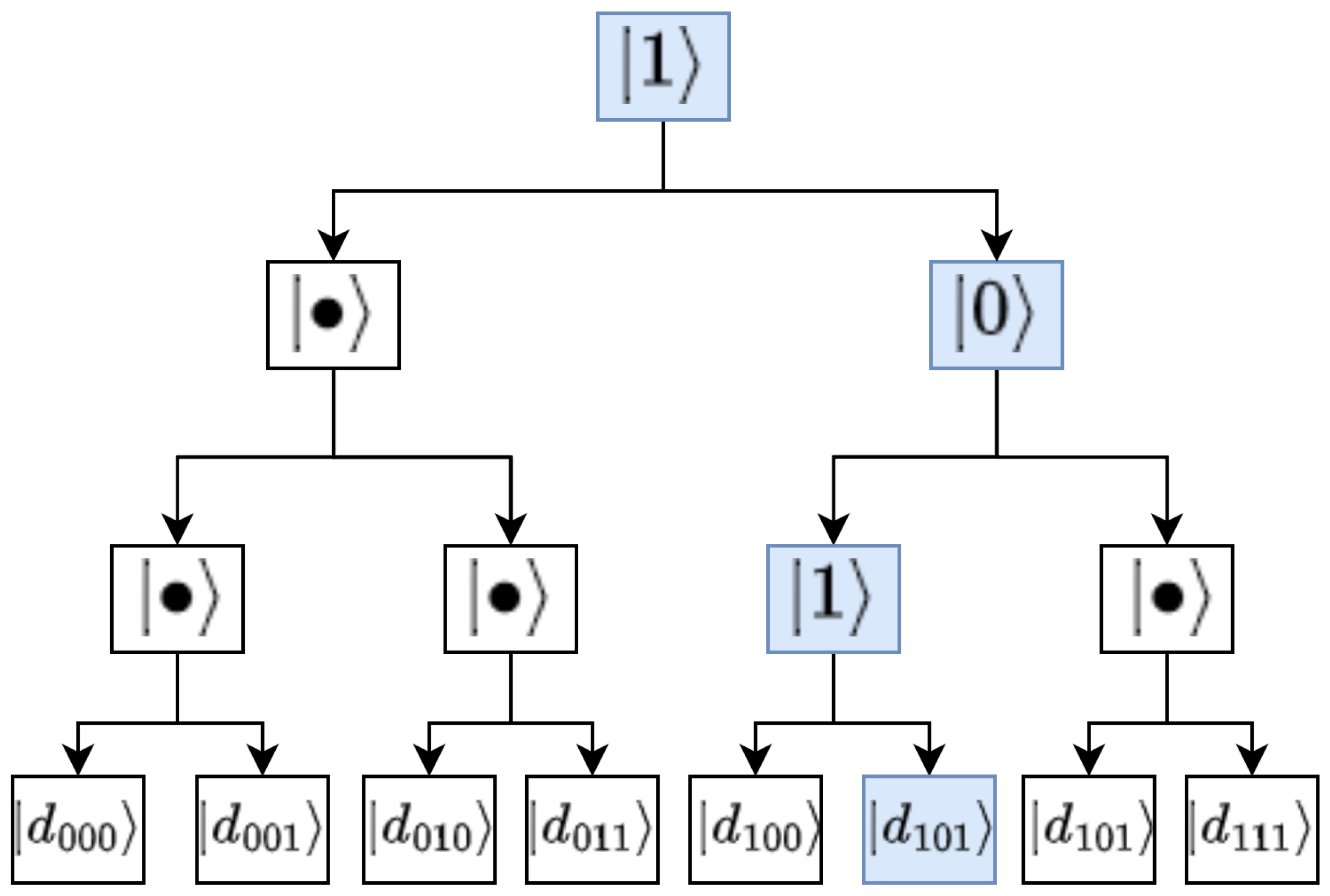
As mentioned, our work is targeted towards the BBA QRAM model. Without going into much detail, the BBA uses three-level systems to build the tree that addresses the registers. Two states are used to denote the path (left–right) and one state is the “wait” state; the path to the target register is obtained by following nodes that have a state different from the “wait” state. Figure 1 depicts an example of an 8-qubit QRAM and how the switches are activated to route to a specific address (see also [19] for a more detailed analysis and how such trees can be simulated in quantum circuits).

In such a scheme, the address register is coupled to the routing qutrits and changes the state from “wait” to the value of the ith qubit, where i denotes the index of the qubit in the index register. For the example of Figure 1, the address register is $|101\rangle$, which sets the states of the corresponding qutrits accordingly. Although a single address is depicted in the example, in general, the QRAM should be able to query a superposition of data registers, according to

$$\begin{array}{c}\hfill {\displaystyle \sum _{j=0}^{2^n}}{\alpha }_j|j\rangle |0\rangle \to {\displaystyle \sum _{j=0}^{2^n}}{\alpha }_j|j\rangle |d_j\rangle \end{array}$$

(1)

where j denotes the addresses of the data registers we want to obtain, ${\alpha }_j$ is the amplitude of the superposition of addresses, and $d_j$ are the contents of the data register indexed at j. For the 8-qubit RAM considered in the above example, and assuming 1-qubit data registers for simplicity, if we wanted to obtain an equal superposition of the registers located at positions indexed at 2 and 7, the QRAM would reply with the superposition:

$$\begin{array}{c}\hfill {\displaystyle \frac{1}{\sqrt{2}}}(|2\rangle \rangle d_2+|7\rangle |d_7\rangle )\end{array}$$

(2)

where Equation (1) is instantiated with $j=2,7$ and with ${\alpha }_j={\displaystyle \frac{1}{\sqrt{2}}}$ for $j=2,7$, and ${\alpha }_j=0$ otherwise. As the operations that are performed on qutrits in the BBA are of the form of single-qutrit rotations to obtain the desired states and controlled operations to change the state based on the incoming state (i.e., to change a qutrit value from waiting to zero or one), the following architecture can be considered a good candidate architecture for implementing a BBA circuit:

• It provides three-level systems with each state having a sufficiently high relaxation $T1$ and dephasing time $T2$ relative to the execution time of a quantum gate;
• It inherently supports gates for the arbitrary initialization of a qutrit state.
• It allows the execution of single- and two-qutrit gates as the ones required by the BBA algorithm.

Giovanetti et al. presented a possible implementation of BBA using photons propagating along a network of coupled cavities that contain trapped atoms [14]. In the regime of transmon systems, Peterer et al. [20] demonstrated that transmons can be excited with sequential pulses $\pi$ up to the fourth excited state, with relaxation times that allow the possibility of using these extra energy states for encoding quantum information. The main aim of the work presented in this paper is to demonstrate that the necessary operations needed for implementing a QRAM based on the BBA can be realized in transmon systems and provide a framework for dynamically finding pulse parameters that realize the necessary transitions.

2. Materials and Methods

The present study leverages two methods for designing the desired pulses:

• A simple qutrit encoding schema that is used to map qutrit states to transmon energy levels. The purpose of this schema is to reduce the number of controlled operations that involve higher-energy states of the transmon.
• A simulation framework that leverages the Qiskit Dynamics [21] and the Boulder Opal [22] libraries to perform an ML-assisted pulse optimization problem, that targets the required logical transitions.

The two methods are presented in the following subsections.

2.1. Qutrit Encoding

Transitions of single-qutrit states can be described by $3\times 3$ unitary operators. In the case of qutrits used for BBA, the most common operations are state preparations and state-based transitions. We identify two kinds of operators:

• The translation operators $T_{i,j}$ that perform a flip between the $|i\rangle$ and $|j\rangle$ basis states of the qutrit; for example, the operator $T_{0,2}$ alters the state $|0\rangle (|2\rangle )$ to $|2\rangle (|0\rangle )$, while leaving the state $|1\rangle$ invariant.
• The permutation operator P, which permutes the states according to $|i\rangle \to |(i+2)mod3\rangle$.

In matrix form, the operators can be given by

$$T_{0,1}=\left(\begin{array}{ccc}0& 1& 0\\ 1& 0& 0\\ 0& 0& 1\end{array}\right),T_{0,2}=\left(\begin{array}{ccc}0& 0& 1\\ 0& 1& 0\\ 1& 0& 0\end{array}\right),T_{1,2}=\left(\begin{array}{ccc}1& 0& 0\\ 0& 0& 1\\ 0& 1& 0\end{array}\right)$$

(3)

for the translation operators, and

$$P_3=\left(\begin{array}{ccc}0& 1& 0\\ 0& 0& 1\\ 1& 0& 0\end{array}\right)$$

(4)

for the permutation operator. Similarly to qubits, controlled operations involve the change of the state of a target qutrit based on the condition of the control qutrit. In direct extrapolation, we can identify the control operation $C{T}_{i,j}$ that performs the operation $T_{i,j}$ on the target qutrit if the control qutrit is in state $|2\rangle$. The implementation of pulses that perform the $T_{i,j}$ transitions can be performed by sending signals that are resonant with the $i\leftrightarrow j$ transition frequency. The permutation operators can be more difficult to implement directly; however, they can be deconstructed by a set of $T_{i,j}$ pulses by using the identity

$$P_3=T_{0,1}{T}_{0,2}$$

(5)

Equation (5) can be validated by direct matrix multiplication; however, it can be instructive to see how it works to cycle qutrit states using qutrit translations. Reading from right to left (to simulate how, as a quantum operator, it would act on a qutrit state) and taking as an example the state $|2\rangle$, the state is first acted on by $T_{0,2}$. Since we consider the state with index equal to 2 (we use a zero-indexed scheme, so the column indexed at position 2 is actually the third column), the relevant column of the $T_{0,2}$ operator is $T_{0,2}^2={\left(\begin{array}{ccc}1& 0& 0\end{array}\right)}^T$ which results in the transition to state $|0\rangle$. We then take operator $T_{0,1}$ and specifically its zero indexed column $T_{0,1}^0={\left(\begin{array}{ccc}0& 1& 0\end{array}\right)}^T$ (since the state is now $|0\rangle$) and observe that it changes the state to $|1\rangle$. This is exactly the same as the operation performed by $P_3$ alone as can be seen by taking Equation (4) and isolating the second-indexed column. For a proof using explicit matrix multiplication, the reader can refer to Appendix A.

Considering the $C{T}_{i,j}$ gates, controlling an operation conditional on the control qutrit being in the first hyper-excited state may involve the design of very complex pulses. The operation itself may be prone to additional error since, generally, coupling operations involve pulses that have a longer duration, and the first hyper-excited state has a lower relaxation time than the two lower ones. Various approaches to surpass this problem can be followed, such as redefining the control gates to involve other control states. For our purposes, however, we follow the simple approach of re-mapping the physical and logical states of the system. For a single transmon, we adopt the following mapping:

$$\begin{array}{cc}\hfill {|0\rangle }_T& \to {|0\rangle }_L\hfill \\ \hfill {|1\rangle }_T& \to {|2\rangle }_L\hfill \\ \hfill {|2\rangle }_T& \to {|1\rangle }_L\hfill \end{array}$$

(6)

where ${|\rangle }_T$ denotes the physical state of the transmon and ${|\rangle }_L$ the logical ones. Consider now a pulse sequence that performs the usual two-qubit CNOT pulse. Such pulses are implemented in modern hardware in such a manner as to ensure that there is minimum leakage to higher excited states; indeed, the fact that the ground and excited states can be separated by the higher ones is one of the key factors that constitute a good quantum processor architecture, such as the one based on transmon systems.

Ignoring the specifics of the pulse and assuming that it operates in the space spanned by the ground and first excited states, the transitions in the CNOT case for the transmon and logical states can be summarized in

Table 1. Correspondence between the physical and logical state evolution under a two-qubit CNOT.

Initial Physical State	Final Physical State	Initial Logical State	Final Logical State
${|00\rangle }_T$	${|00\rangle }_T$	${|00\rangle }_L$	${|00\rangle }_L$
${|01\rangle }_T$	${|01\rangle }_T$	${|02\rangle }_L$	${|02\rangle }_L$
${|02\rangle }_T$	${|02\rangle }_T$	${|01\rangle }_L$	${|01\rangle }_L$
${|10\rangle }_T$	${|11\rangle }_T$	${|20\rangle }_L$	${|22\rangle }_L$
${|11\rangle }_T$	${|10\rangle }_T$	${|22\rangle }_L$	${|20\rangle }_L$
${|12\rangle }_T$	${|12\rangle }_T$	${|21\rangle }_L$	${|21\rangle }_L$
${|20\rangle }_T$	${|20\rangle }_T$	${|10\rangle }_L$	${|10\rangle }_L$
${|21\rangle }_T$	${|21\rangle }_T$	${|12\rangle }_L$	${|12\rangle }_L$
${|22\rangle }_T$	${|22\rangle }_T$	${|11\rangle }_L$	${|11\rangle }_L$

.

As can be seen in Table 1, the logical state of the target qubit makes the transition ${|0\rangle }_L\leftrightarrow {|2\rangle }_L$ when the logical state of the control qubit is $|2\rangle$. This corresponds to the operation of $C{T}_{0,2}$, which in explicit matrix notation can be described as

$$\begin{array}{c}\hfill C{T}_{0,2}=\left(\begin{array}{ccccccccc}1& 0& 0& 0& 0& 0& 0& 0& 0\\ 0& 1& 0& 0& 0& 0& 0& 0& 0\\ 0& 0& 1& 0& 0& 0& 0& 0& 0\\ 0& 0& 0& 1& 0& 0& 0& 0& 0\\ 0& 0& 0& 0& 1& 0& 0& 0& 0\\ 0& 0& 0& 0& 0& 1& 0& 0& 0\\ 0& 0& 0& 0& 0& 0& 0& 0& 1\\ 0& 0& 0& 0& 0& 0& 0& 1& 0\\ 0& 0& 0& 0& 0& 0& 1& 0& 0\end{array}\right)\end{array}$$

(7)

The other controlled operations can be obtained by using the identities

$$\begin{array}{c}\hfill C{T}_{0,1}={(I_3\otimes P_3)}^{2}C{T}_{0,2}(I_3\otimes P_3)\\ \hfill C{T}_{1,2}=(I_3\otimes P_3)C{T}_{0,2}{(I_3\otimes P_3)}^2\end{array}$$

(8)

where $I_3$ is the three-dimensional identity matrix and the symbol ⊗ denotes tensor products. Similarly to the interpretation given for Equation (5), the identities can be logically deducted by observing that the $(I_3\otimes P_3)$ operators act on the second qutrit subspace to alter its state accordingly, before and after the operation of the $C{T}_{0,2}$ operator. As an example, consider the application of the $C{T}_{1,2}$ operator to a target qutrit in state $|2\rangle$. If the control qutrit is not in state $|2\rangle$, then the $C{T}_{0,2}$ operator will have no effect and, according to the second equation of Equation (8), the permutation operator will be applied three times to the state, performing the transitions $|2\rangle \to |1\rangle \to |0\rangle \to |2\rangle$, effectively leaving the state invariant. If, however, the control qutrit is in state $|2\rangle$, then after the second permutation, which sends the state of the target qutrit to $|0\rangle$, the $C{T}_{0,2}$ operator will alter its state to $|2\rangle$. The final permutation will then send state $|2\rangle$ to state $|1\rangle$, thus performing the equivalent of a $C{T}_{1,2}$ operation. We shall not exhaust all the other cases; the reader can refer to Appendix A for the computation that derives all the $C{T}_{i,j}$ matrices using the identities of Equation (8).

Under all of the assumptions above, we can see that the desired logical operations can be obtained by pulses that involve only single-qutrit $T_{i,j}$ transitions and only one two-qutrit gate that can be implemented by applying existing approaches that realize the two-qubit CNOT gate.

2.2. Pulse Optimization

The methodology for designing efficient pulses for state preparations and controlled state transitions relies on leveraging existing techniques for accessing the higher-energy states of transmon systems, while also avoiding performing controlled operations that involve higher excited states both as controls and as targets to reduce the computational error. For estimating pulse parameters, we adopt the following Hamiltonian (see, for example, the overview of Kratz et al. [23] for a complete description of how to describe the static and interacting terms of transmon Hamiltonians):

$$\begin{array}{cc}\hfill H& ={\displaystyle \sum _{i=\{0,1\}}}{v}_i{a}_i^{†}{a}_i\hfill \\ \hfill & +{\displaystyle \frac{1}{2}}{\displaystyle \sum _{i=\{0,1\}}}{\alpha }_i{a}_i^{†}{a}_i(a_i^{†}{a}_i-I)\hfill \\ \hfill & +{\displaystyle \sum _{i=\{0,1\}}}{d}_i\left(t\right)(a_i+a_i^{†})\hfill \\ \hfill & +J{\displaystyle \prod _{i=\{0,1\}}}(a_i+a_i^{†})\hfill \end{array}$$

(9)

where the first two rows refer to the free Hamiltonians of the two transmons with frequencies $v_0$ and $v_1$ and with anharmonicities equal to ${\alpha }_0$ and ${\alpha }_1$. $a_i^{†}$($a_i$) are the creation(annihilation) operator for qutrit i. $d_i\left(t\right)$ refer to the drive signals that can be applied to the transmons to achieve control; these can be further decomposed to the Rabi strengths and the time signals themselves, but we keep these two terms together for simplicity. Factors of $2\pi$ are omitted for simplicity. Finally, the coupling of the systems with coupling strength J is included in the final row. While a perfect transmon could be described by the Pauli operators, we introduce the more generic annihilation and creation operators both to access the higher-energy states and to ensure that unwanted leakage to other states is modeled appropriately. To this end, we adopt a 5-level oscillator to accommodate both cases.

For the one-qutrit pulses, the following assumptions are made:

• Relaxation and dephasing times have been ignored as a first approximation. Our main focus is to establish errors due to the leakage to unwanted states, which are typically introduced due to imperfect calibrations or crosstalk terms. These are modeled in our Hamlitonian.
• A maximum power of 1.0 is imposed on our simulations. Although driving a transmon from its ground state directly to the second excited state is, in theory, possible, it may involve the realization of strong pulses so that current architectures may not possess (the IBM Quantum Platform for example, has an upper limit of a pulse amplitude equal to one; the value can be overridden but only for simulations).

Under those assumptions, the process for constructing the $T_{i,j}$ pulse is the following (for this section, the indices of the T pulses refer to physical states and not logical ones):

• Perform a Rabi experiment to estimate the amplitude of the pulse.
• Drive the qutrit and obtain the fidelity.
• For the $T_{0,2}$ pulse especially, use the two calibrated $T_{0,1}$ and $T_{1,2}$ pulses in sequence (here, and for all single-qutrit operations described in the present section, we refer to the physical operations that alter the ${|\rangle }_T$ states of Equation (6)).

Using a frequency of 4.86 GHz for the first transmon and an anharmonicity of −320 MHz (these, and all the other system parameters, are taken from the existing Almaden backend from IBM Quantum Platform to make the experiments more realistic), the system is simulated using the Qiskit Dynamics library. A five-level oscillator is used to model the possibility of leakage to unwanted higher-energy states. For simplicity, constant pulses are used. For modulating the pulses to signals, we use the $v_0+{\alpha }_0$ frequency as a carrier frequency for the transition $T_{0,2}$. Figure 2 shows the mixer output of the two combined signals that performs a $T_{0,2}$ transition. A Rabi strength of 0.21 is used. (Here, we use the normalized dimensionless units that Qiskit uses. The exact strength and units of the signal that a qubit would ‘feel’, is dependent on the physical realization of the qubit and of any transformations that the signal converter would do. For a flux qubit, for example, the signal would have to be converted to currents. Qiskit hides these details by exposing a dimensionless amplitude parameters and performing the underlying signal conversions.) The dimensionless coupling parameter is taken to be equal to $J=2\times {10}^{-2}$.

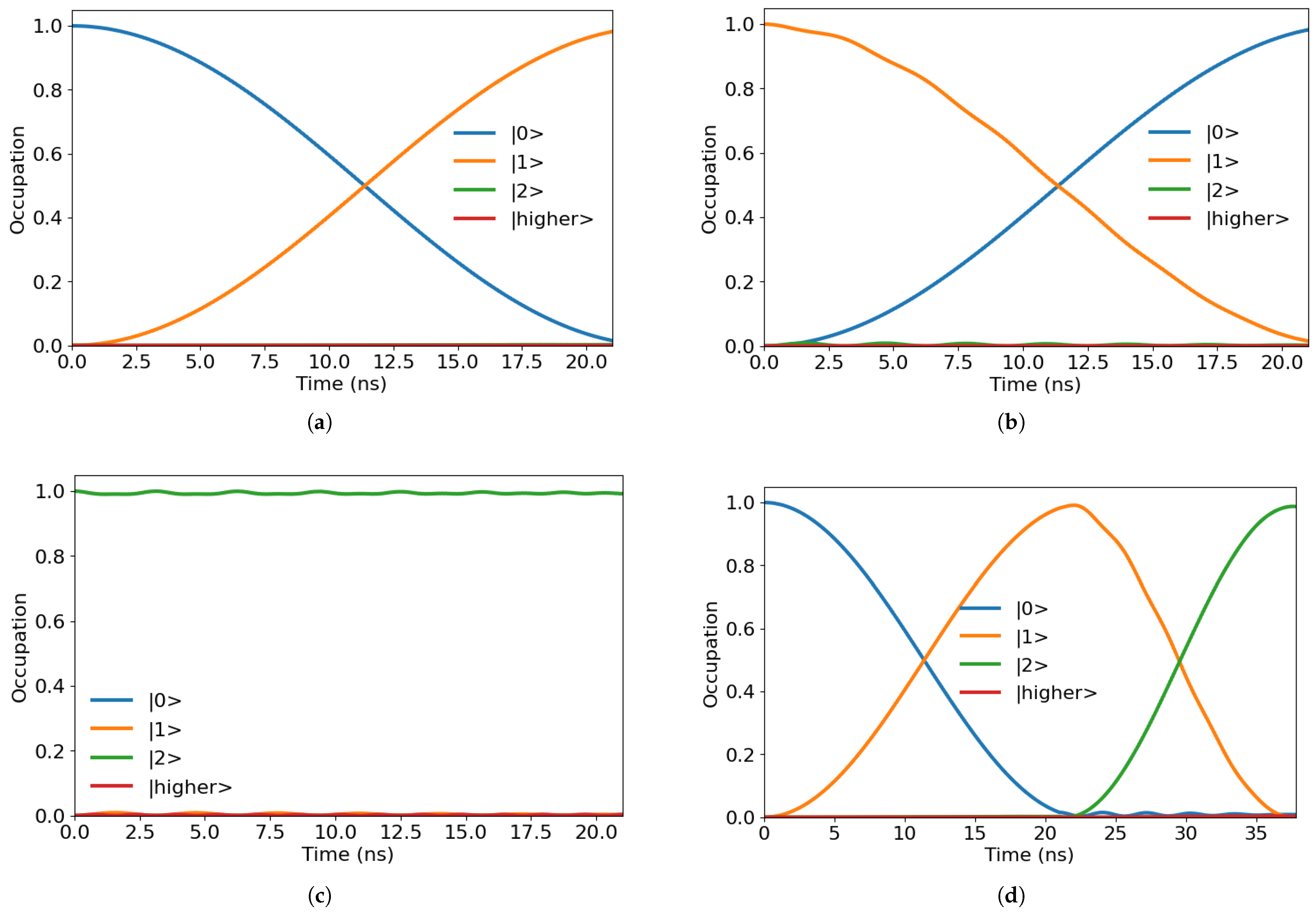
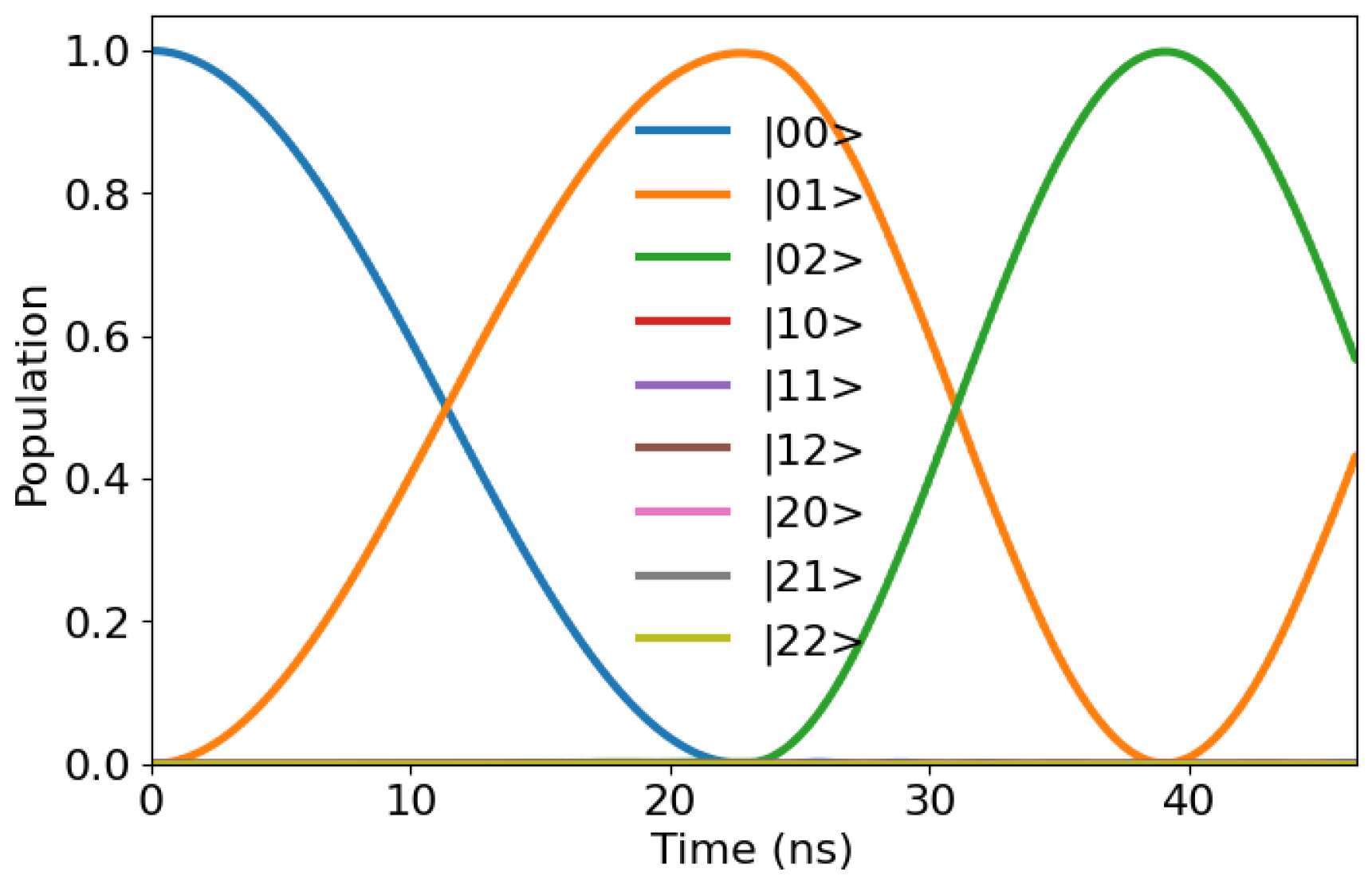
In Figure 3, some indicative examples of how states are evolved are depicted for the case of the first qubit. As shown, $T_{0,1}$ swaps the populations of $|0\rangle$ and $|1\rangle$ states, while leaving state $|2\rangle$ invariant. The $T_{0,2}$ pulse, on the other hand, performs the $|0\rangle \to |2\rangle$ transition as expected.

Regarding the pulses’ accuracies, these are estimated by calculating the corresponding infidelities, which are obtained by comparing the relative populations between the target and the computed states. More specifically, the infidelities $in{f}_{T_{i,j}}$ are computed using the type $in{f}_{T_{i,j}}=1-f_{T_{i,j}}$, where $f_{T_{i,j}}$ are the Hellinger fidelities of the count distributions. Removing the operator subscripts for clarity, for each operator, the Hellinger fidelities are computed by

$$\begin{array}{c}\hfill f={({\displaystyle \sum _{i=0}^5}\sqrt{q_i{p}_i})}^2\end{array}$$

(10)

where $q_i$ and $p_i$ denote the final populations of the simulated and ideal states, respectively, for all possible outcomes. The possible outcomes are $i=\{0,1,2\}$ for the possible qutrit states and $i=\{4,5\}$ to include the possibility of unwanted leakage to even higher-energy states. (It can be seen that, when comparing to ideal distribution, the sum degenerates to a single term since $p_i=0$ for all populations not belonging to the target state. However, the Hellinger fidelity thus defined is used since it can be directly computed by using Qiskit’s library and can be easily extended to more general cases.)For a description of the basic setup and simulation parameters of the experiment, the reader can refer to Appendix B.

Table 2. Pulse infidelities for the $T_{i,j}$ pulses.

Pulse	Infidelity
$T_{0,1}$	9.81 × ${10}^{-7}$
$T_{1,2}$	9.86 × ${10}^{-7}$
$T_{0,2}$	1.90 × ${10}^{-6}$

shows the calculated infidelities for the three pulses. Note that the operations are the physical ones that correspond to the energy levels of the transmon.

It is to be noted that even when the second qutrit is taken into account, noises due to crosstalk can be minimal when the frequencies, anharmonicities, and couplings are appropriately defined. Figure 4 for example, shows the evolution of the first qutrit under a $T_{0,2}$ gate, where the second qutrit involved has a frequency equal to $v_1$ = 4.97 GHz, and an anharmonicity of ${\alpha }_1$ = −320 MHz, in the presence of crosstalk due to the coupling.

2.3. Two-Qutrit Gates

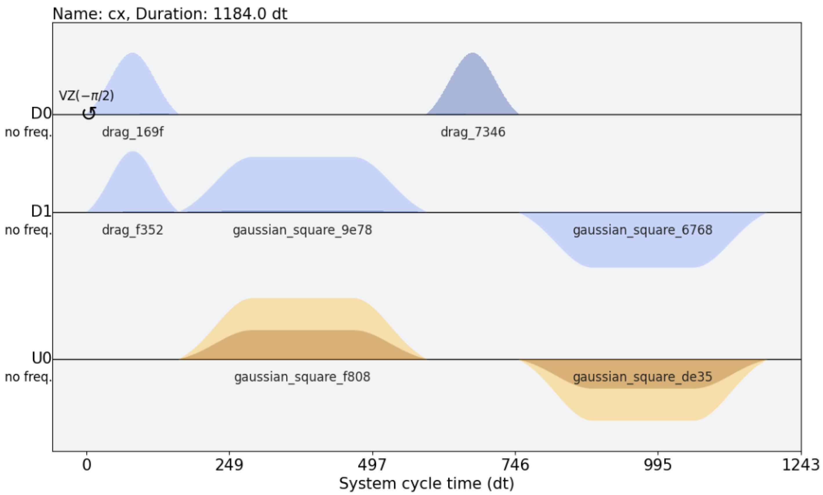
As we have seen in Section 2.1, controlled qutrit operations can be reduced to a series of $T_{i,j}$ and 2-qubit $CNOT$ operations with the appropriate encodings. Designing a pulse for performing a CNOT in transmon can then be seen as a trivial problem since we can calibrate existing pulses that modern quantum architectures offer. Figure 5, for example, shows a schedule that performs a CNOT gate on the Valencia processor of the IBM Quantum Platform.

The main issues of obtaining such pulses out of the box, calibrating them, if needed, and applying them for qutrit manipulation according to the schematics presented are the following:

• CNOT gates are rarely truly native gates in transmon architectures. For transmons with fixed frequencies, they are usually based on the cross-resonance gates, which are implemented by driving the control qubit with the target’s qubit frequency. Calibrating such a CNOT may involve processes that are not directly applicable to processors that expose different gate-sets (e.g., an ECR gate) and additional calibration processes may need to be applied.
• As is usual with many transmon architectures, arbitrary rotations around the Z axis by and angle $\theta$ (realized $Rz\left(\theta \right)$ gates) are implemented with virtual pulses (i.e., changes of reference frames) that must be applied across channels in the case of a CNOT gate. When higher-frequency states are involved, these rotations may need to be recalculated to accommodate for the additional wiggle factors of the expanded basis set.

To this end, we opt to adopt a more general approach in which a cross-resonance gate can be defined using the characteristics of the underlying Hamiltonian. If such a schedule is found, then a CNOT gate can be obtained by

$$\begin{array}{c}\hfill CNOT={(I\otimes Z)}^{-1/2}{(X\otimes Z)}^{-1/2}{(X\otimes I)}^{-1/2}\end{array}$$

(11)

where ${(X\otimes Z)}^{-1/2}$ is the maximally entangling cross-resonance gate obtained from the general $R_{xz}\left(\theta \right)=exp(-i{\displaystyle \frac{\theta }{2}}X\otimes Z)$ gate.

The right term corresponds to a one-qubit $\sqrt{X}$; in the gate set used in our model, this corresponds to a $\sqrt{T_{0,1}}$ gate, which can be performed by the same pulse used for the $T_{0,1}$ if it is applied for half a duration of the pulse.

The leftmost term corresponds to a one-qubit $\sqrt{Z}$ gate. $R_z$ rotations, of which $\sqrt{Z}$ is a special case, can be performed by different methods in transmon systems. If an external pulse $V\left(t\right)$ of the form

$$V\left(t\right)=\mathsf{\Omega }cos({\omega }_{d}t-\varphi )$$

(12)

is applied to a transmon qubit, then the total Hamiltonian of the qubit can be written as follows (we use the Pauli matrices for simplicity since we focus for now to two-level systems; in addition, we remove all ℏ factors for convenience):

$$H=-{\displaystyle \frac{{\omega }_0}{2}}{\sigma }_z+V\left(t\right){\sigma }_x$$

(13)

It can be shown that by changing to the frame that rotates with the qubit’s frequency and under the rotating wave approximation, the rotating Hamiltonian can be expressed as

$$H_R={\displaystyle \frac{\mathsf{\Omega }}{2}}\left(\begin{array}{cc}0& e^{i\mathsf{\Delta }t-\varphi }\\ e^{-i\mathsf{\Delta }t-\varphi }& 0\end{array}\right)$$

(14)

where $\mathsf{\Delta }$, assuming that we are studying the 0-indexed qubit, is equal to $\mathsf{\Delta }={\omega }_d-{\omega }_0$. For $\mathsf{\Delta }=0$, we have resonant pulses that perform rotations around the X axis; all single-gate pulses that we have studied thus far fall under this category, with the main difference being that they are performed on systems that have more than two states.

An $R_z$ rotation can be performed via the following:

• Use a slightly off-resonant pulse to introduce a phase difference between the qubit’s state vector and the rotating frame.
• Use the $\varphi$ angle in Equation (14) to place the rotation axis parallel to the z axis.

Many platforms, such as the IBM Quantum Platform, use the second approach (please also refer to https://docs.quantum.ibm.com/api/qiskit/qiskit.circuit.library.RZGate (accessed on 6 February 2025)), as this phase change can be performed by simply adjusting the phase of the pulses; such frame changes, also referred to as virtual gates, can be performed classically via the signal generators by introducing the appropriate delays. At the cost of having to track the delays and changes across the channels via the program that implements the pulse schedule of the whole quantum program, this approach implements $R_z$ pulses with effectively zero duration and error (for a complete treatise of how to implement virtual $R_z$ gates and how update the phases to take into account subsequent multi-qubit interactions, see [24]).

In our implementation, arbitrary $R_z$ rotations are seldom needed for qutrit control that is typically encountered in BBA circuits, while, due to the extra computational states used, the extra wiggle factors of these states may increase the complexity of bookkeeping the phase delays. We are therefore using a simple calibration process for identifying optimum pulse parameters for implementing the

$$\sqrt{Z}=\left(\begin{array}{cc}1& 0\\ 0& i\end{array}\right)$$

(15)

gate by using the Boulder Opal framework. The Boulder Opal framework offers a vast array of functionalities for computing optimal parameters for quantum control and for simulating systems, including, among others, superconducting qubits [25].

In similar fashion to the one-qutrit gates and the simulations based on Qiskit Dynamics, we define a two fixed-frequency transmon system and use the same frequency, anharmonicity, and coupling strengths. We then define the target operation and run the Boulder Opal optimizer to generate a pulse that is being composed by piecewise-constant segments that minimize the gate infidelity. Boulder Opal calculates the operational infidelity of a gate by using the formula:

$$Inf=1-{\left|{\displaystyle \frac{Tr\left(U_T^{†}U\right)}{Tr\left(U_T^{†}{U}_T\right)}}\right|}^2$$

(16)

where $U_T$ is the target operator (in our case, these operators are the ${\left(XZ\right)}^{-1/2}$ two-qutrit operator operating in the subspace of the two lowest energy states and $\sqrt{Z}$ operating in the subspace spanned by the two lowest energy states of the first qutrit) and the U is the operator that corresponds to the pulses computed by Boulder Opal using gradient optimization (the reader can refer to Appendix C for a brief description of how Boulder Opal can be used to instantiate problems and compute infidelities). The optimized pulse achieves an infidelity equal to 9.58 $\times {10}^{-7}$ for the $\sqrt{Z}$ gate, while the one computed for the ${\left(XZ\right)}^{-1/2}$ following the same methodology achieves an infidelity equal to 1.23 $\times {10}^6$. The same methodology can be used for the ${\left(XZ\right)}^{-1/2}$ gate. See Figure 6 for a plot of the computed pulses. For each of the two pulses, the calculated Rabi amplitudes $\mathsf{\Omega }$ are plotted together with the corresponding phase $\varphi$ (in contrast to the Qiskit experiment, Boulder Opal computes directly the relevant pulse amplitudes based on the provided Hamiltonian, and as such, these are depicted with explicit units of MHz, which are typical units for quantum systems coupled to microwave pulses).

3. Results

This paper presented a methodology for designing efficient pulses on transmon systems that realize gates that are encountered in the Bucket Brigade Algorithm for QRAM. It focused on transitions between basis states and controlled operations for conditionally altering the state of one qutrit based on the other. In order to avoid the need of designing pulses that control the first hyperexcited state ($|2\rangle$), proper encodings were used, together with additional pulses of one qutrit.

Ignoring the relaxation and dephasing times, and focusing only on errors introduced by the Hamiltonian dynamics, such as crosstalk terms, the infidelities theoretically computed by the simulation are depicted in

Table 3. Correspondence between physical and logical state evolution under a two-qubit CNOT.

Gate	Pulse Realization	Infidelity
$T_{0,2}$	$T_{0,2}$	9.81 $\times {10}^{-7}$
$T_{1,2}$	$T_{1,2}$	9.87 $\times {10}^{-7}$
$T_{0,1}$	$T_{1,2}{T}_{0,2}$	1.90 $\times {10}^{-6}$
$P_3$	$T_{0,1}{T}_{0,2}$	3.70 $\times {10}^{-6}$
$Z^{-1/2}$	$Z_{0,1}^{-1/2}$	9.58 $\times {10}^{-7}$
$X^{-1/2}$	$T_{0,2}^{-1/2}$	9.81 $\times {10}^{-7}$
$X{Z}^{-1/2}$	$X{Z}^{-1/2}$	1.30 $\times {10}^{-6}$
$C{T}_{0,2}$	${\left(IZ\right)}^{-1/2}{\left(XZ\right)}^{-1/2}{\left(XI\right)}^{-1/2}$	2.81 $\times {10}^{-6}$
$C{T}_{0,1}$	$\left(I_3{P}_3\right)C{T}_{0,2}{\left(I_3{P}_3\right)}^2$	3.23 $\times {10}^{-5}$
$C{T}_{1,2}$	${\left(I_3{P}_3\right)}^{2}C{T}_{0,2}\left(I_3{P}_3\right)$	3.63 $\times {10}^{-5}$

, where the indices of the gates correspond now to the logical states introduced in Table 1. Each gate is described by its relevant pulse. For economy, composite gates that are performed by a series of pulses are listed by their gate names in subsequent pulse schedules after they are first introduced (for example, the $T_{0,1}$ gate is described as a series of $T_{1,2}{T}_{0,2}$ pulses in the third row, but is subsequently listed as $T_{0,1}$ in pulse schedules). Furthermore, the gates $\sqrt{X}$, $\sqrt{Z}$ and the maximally entangling cross-resonance gate that act on the qubit subspace are listed as gates though, strictly speaking, they are not part of the model’s gate set. This happens to list their infidelity separately and for better visualizing the pulse schedules.

All infidelities, except the last three, were obtained by performing the simulations described in Section 2. The last three were obtained by applying the pulse parameters in Boulder Opal and taking the average of infidelities of an ensemble of input states. The results agree with what was expected on the basis of the constituent pulse infidelities.

4. Discussion

The results suggest that under the appropriate logical mappings, the qutrit control operations required to operate addressing switches in QRAM based on the BBA architecture can be realized by using the same entangling gates as the one used for quantum computation based on qubits. Although this was achieved at the extra cost of some additional single-qutrit gates, we demonstrated that single-qutrit transitions can be easily defined and calibrated for the case of qutrits that are realized using the energy levels of transmon systems. A methodology for using existing tools to optimize the pulses needed was also presented; this pipeline can be parametrized both in terms of the transmon parameters (e.g., resonance frequencies and anharmonicities) and in terms of the definition of the native gates used, which can be set as target operators that the parametrized signals must approximate. The results suggest that using transmon systems to address quantum registers under the Bucket Brigade scheme may be a promising technique for implementing a QRAM based on BBA in transmons. However, there are various considerations and further steps that need to be taken before the model can be adopted experimentally.

4.1. Noise Suppression and Mitigation

While the infidelities computed seem promising for realizing the described qubit control, these were computed by only minimizing errors introduced by the dynamics of the Hamiltonian, such as leakage to unwanted states or crosstalk terms that need to be canceled for the cross-resonance gate to be effective. Couplings to the external environment that introduce relaxation and dephasing were not considered; these, however, are an important source of error in current NISQ architectures. Future work will focus on applying error mitigation techniques and validating the results on real quantum hardware. Among others, we will take advantage of the Fire Opal [26] package that has demonstrated good results in applying error suppression techniques and that provides a good number of integrations with hardware providers such as those of the IBM Quantum Platform.

4.2. Transmon Connectivity

Transpiling a logical quantum circuit into the native instruction set of a quantum processor may drastically increase the depth of the resulting circuit, also called the Instruction Set Architecture or ISA circuit. The efficiency of transpiling greatly depends on the characteristics of the logical quantum circuit, the native instruction set, and the qubit connectivity of the quantum processor; an efficient algorithm that produces small native circuits for a specific class of problems may perform poorly for other classes even in transpiled in the same quantum processor.

In the case of our model, the gates are implemented at the pulse level; as such, translation to the native gate set is straightforward as long as the quantum hardware supports access at the pulse level. Mapping the logical qutrits to the layout of the backend, however (the so-called routing stage of transpilation), is an entirely different matter, as this often involves quantum state transfers which are typically implemented via $SWAP$ gates for qubits. Designing such pulses with sufficiently low infidelity is one of the main goals of our future work. This work will be supplemented with the investigation of routing techniques for qutrit circuits, with the aim of possibly reducing the required amount of qutrit $SWAP$ operations.