Fast Temperature Field Extrapolation Under Non-Periodic Boundary Conditions

Abstract

The rapid and accurate prediction of temperature fields in complex structures remains a significant challenge in thermal engineering. Experimental approaches often struggle to provide comprehensive data, while traditional full-order numerical methods are hindered by their excessive computational demands. This study addresses these limitations by developing a novel reduced-order extrapolation method that integrates proper orthogonal decomposition (POD) with the finite volume method (FVM). We demonstrate the efficacy of our approach through its application to multilayered thermally unstable structures under non-periodic boundary conditions. The results reveal exceptional performance in both prediction accuracy and computational efficiency. When validated against experimental data and conventional FVM results, our method achieves a maximum relative error of less than 5% while delivering a remarkable computational speed-up of more than 1400 times when running complex explosive structure simulations. Notably, our analysis uncovers a critical limitation of POD: increasing the number of modes does not proportionally enhance the prediction accuracy, due to inherent methodological constraints. This innovative strategy offers promising potential for real-time temperature monitoring and thermal protection in advanced engineering systems, particularly for complex devices requiring precise thermal management.

1. Introduction

Engineering equipment is often faced with complex and variable operation conditions, such as anomalous thermal stimuli, force stimuli, and electromagnetic stimuli [1,2,3]. In particular, roughly 55% of the failures seen in equipment are caused by severe thermal stimuli, and the thermal field analysis of equipment is critical [4,5]. It is impossible to obtain comprehensive and accurate thermal field data through experiments using intrusive means. Theoretically, numerical heat transfer theory can be used to simulate the temperature field by establishing a heat transfer model for any complex structure [6,7,8]. However, a full-order model such as this entails a large-scale system of algebraic equations, which requires huge computational resources [9,10]. The tedious calculation process is a great obstacle to the need for rapid thermal analysis and optimization, so it is necessary to introduce a reduced-order model to accelerate their calculation.

The proper orthogonal decomposition (POD) method is one of the most commonly used methods in the field of model order reducing [11,12,13], which is able to extract a set of low-dimensional optimal POD bases from the huge physical field of its target, after which this set of optimal POD bases is used to approximate the original physical field. The method was originally proposed by Pearson [14] in 1901 and is now widely used in fields such as signal analysis, statistics, meteorology, and fluid mechanics [15,16,17]. Taking the field of fluid dynamics as an example, Lumley [18] first applied the POD method to turbulence research in 1967 when identifying coherent structures in the flow field, and he processed the spatial correlation matrix directly. The method he used was named the direct POD method. The dimension of the spatial correlation matrix is very large, being comparable to the scale of the number of meshes, which severely limits the application of the POD method. To address such problems, Sirovich [19] proposed the snapshot POD method in 1987, replacing the spatial correlation matrix with the temporal correlation matrix when the spatial dimension was larger than the temporal dimension, which greatly reduced the computational cost. Since then, the POD method has been developed for use in many contexts. In the field of heat transfer, Hazenberg et al. [20] established a POD–Galerkin reduced-order model for the unsteady thermal conductivity problem of a two-dimensional flat plate, which reduced the degrees of freedom of the system from 1452 to 5. Raghupathy et al. [21] developed the boundary-independent POD reduced-order model. Georgaka et al. [22] coupled the POD-Galerkin method with the Navier–Stokes equations for the unsteady flow and heat transfer problem of a three-dimensional T-tube. The results showed that their method was hundreds of times faster than the full-order model. Hu et al. [23] combined the POD reduced-order method with cubic spline interpolation to study the cross-scale flow and heat transfer in an air-cooled island, which significantly reduced the computational cost. He et al. [24] combined the POD reduced-order method with deep learning to construct the relationship of POD mode coefficients with different operating conditions for a steam generator. However, most of the studies mentioned above are multi-case problems, the purpose of which is to use the known solutions of parts of case studies for POD reduced-order problems to obtain the solutions for other scenarios [25,26]. The method consumes huge resources for the computation of numerical samples and it involves repetitive computation in terms of the time scales. Luo et al. [27,28,29] proposed a reduced-order extrapolation algorithm based on the POD method, which is a method that uses the known solution to quickly calculate the solution for future scenarios under the same operating conditions. It is of great importance to speed up the calculation of transient equations. There have been reduced-order extrapolation algorithms combining the POD method with various types of numerical methods such as the finite difference method, finite element method, finite volume method, and boundary element method [30,31,32,33,34,35]. Unfortunately, most of the algorithms proposed by researchers are based on two-dimensional structures and use structured grids. It is difficult to calculate the temperature field of a three-dimensional structure under complex boundary conditions [36,37,38,39], although progress has been made by researchers in some areas, exploring a combination of Green’s function, the element-free Galerkin (EFG) method, and so on [40,41,42].

In this work, the finite volume method using an unstructured grid has been selected to be combined with the POD method, thereby constructing a rapid computational model for the POD-FVM reduced-order extrapolation of heat transfer problems. We applied it to the thermal field analysis of a multilayer thermally unstable structure under pulsating flame boundary conditions. The proposed method solves the coupling problems of complex structures, complex properties, and complex boundaries. Using the unstructured mesh model for the reduced-order computation strongly promotes the application of the POD reduced-order extrapolation method. It is meaningful for the monitoring and prediction of the temperature field of the device and for thermal protection.

2. Methodology

2.1. POD Reduced-Order Method

As an efficient method of order reduction, the POD technique can use fewer POD modes to describe the original physical field well. The combination of POD and a numerical method can better reduce the degree of freedom of the algebraic equations system of the full-order model to the two-digit level, thus greatly reducing the numerical calculation time and meeting the need for fast calculation or fast prediction.

Before using the POD order reduction method, appropriate sample data should be prepared and assembled into a transient matrix. Since this paper mainly studies the solution of unknown time periods in the calculation of an unsteady temperature field, the sample data collected came from discrete data on a known time scale. The temperature $T(x,t_i)$ of the unsteady temperature field at a specific time is recorded as a set of temperature snapshots, then the temperature snapshots taken at different times are assembled into a temperature transient image matrix $T(x,t)$.

Firstly, finite orthogonal series expansion is used to approximate the original system, namely:

$$T(x,t)\approx {\displaystyle \sum _{i=1}^N{\alpha }_i(t){\phi }_i}(x)=T^{\prime }(x,t)$$

(1)

In the formula, $T^{\prime }(x,t)$ represents the POD’s approximate solution of the temperature field system, $\alpha$ represents the coefficient of a linear combination of the POD modes, $\phi$ represents the POD modes, and N represents the number of intercepted POD modes.

The POD is used to extract low-order important features from the data in the process of system change, and then a combination of fewer POD modes and coefficients is used to reconstruct the complex physical process. The criterion of POD mode selection is that the reserved modes can achieve the best approximation to the temperature field, namely, the error between the temperature transient matrix and the approximate temperature transient matrix is minimal. The most widely used approach to solve the above problem is the L₂-norm, also known as the least-square estimation, which can be formulated as follows:

$$T^{\prime }(x,t)=\arg \underset{{\phi }_i(x)}{\min }{‖T(x,t)-{\displaystyle \sum _{i=1}^N{\alpha }_i(t){\phi }_i(x)}‖}_2^2$$

(2)

The truncation error between the selected POD modes’ reconstructed temperature field matrix $T^{\prime }(x,t)$ and the original temperature field matrix $T(x,t)$ can be expressed as follows:

$$error={\displaystyle \sum _{i=N+1}^{\infty }{\phi }_i^{{\rm T}}(T^{\prime }{T}^{\prime {\rm T}}){\phi }_i}$$

(3)

The Lagrange multiplier ${\pi }_i$ is introduced to establish the Lagrange function as:

$${\phi }_i^{{\rm T}}R{\phi }_i={\pi }_i$$

(4)

As can be seen from the above formula, the Lagrange multiplier ${\pi }_i$ is the eigenvalue of the real symmetric matrix R and ${\phi }_i$ is the eigenvector of the real symmetric matrix R. According to the properties of the real symmetric matrix, it can be seen that the eigenvalues of the matrix R are real numbers and the eigenvectors are orthogonal to each other. Therefore, the truncation error can be expressed as:

$$error={\displaystyle \sum _{i=N+1}^{\infty }{\phi }_i^{{\rm T}}}R{\phi }_i={\displaystyle \sum _{i=N+1}^M{\pi }_i}$$

(5)

where M is the number of matrix eigenvalues.

As can be seen from the above formula, the truncation error can be calculated by the sum of the (M-N) eigenvalues of the real symmetric matrix R. The eigenvalues of the real symmetric matrix R are arranged from the largest to the smallest, and we select the first N largest eigenvalues in order to minimize the sum of the truncated unreserved eigenvalues. Therefore, the eigenvectors corresponding to the retained eigenvalues constitute the optimal orthogonal mode set of the POD. The selection rules are as follows:

$$N=\arg \min \{I(N):I(N)\ge \gamma \}$$

(6)

In the formula, $I(N)$ is:

$$I(N)={\displaystyle \sum _{i=1}^N{\pi }_i}/{\displaystyle \sum _{i=1}^M{\pi }_i}$$

(7)

where the $\gamma$ refers to accumulated energy, which represents the proportion of the eigenvalues of the optimal POD mode set retained after interception and the sum of the eigenvalues in the original mode set. Sirovich recommends $\gamma \ge 99\%$, but this can be adjusted appropriately according to the specific research problem. The main feature of the POD method is that it can provide the best approximation of the original system in the current data length in terms of energy.

2.2. FVM for Unstructured Grid

The spatial discrete method of an unstructured grid has strong adaptability for complex structures, but because it does not consider the regular topological relationship between nodes and elements, the obtained grid data is disordered, and it is then necessary to artificially process the grid data to obtain the relationship between adjacent nodes and adjacent elements. In order to facilitate the combination of the POD method and the unstructured-grid finite volume method, this study employs a fully tetrahedral unstructured mesh for three-dimensional structures.

Considering these three-dimensional, invariable physical properties, we use the unsteady heat transfer equation:

$$\rho c{\displaystyle \frac{\mathsf{\partial }T}{\mathsf{\partial }t}}=\lambda \left({\displaystyle \frac{{\mathsf{\partial }}^{2}T}{\mathsf{\partial }{x}^2}}+{\displaystyle \frac{{\mathsf{\partial }}^{2}T}{\mathsf{\partial }{y}^2}}+{\displaystyle \frac{{\mathsf{\partial }}^{2}T}{\mathsf{\partial }{z}^2}}\right)+s$$

(8)

where $\rho$ is the density $({\mathrm{kg}/\mathrm{m}}^3)$, $c$ is the specific heat capacity $(\mathrm{J}/(\mathrm{kg}\cdot \mathrm{K}))$, $\lambda$ is the thermal conductivity $(\mathrm{W}/(\mathrm{m}\cdot \mathrm{K}))$, and $s$ is the generalized internal heat source $({\mathrm{W}/\mathrm{m}}^3)$.

The unstructured grid discrete form of the heat conduction equation is derived using the concept of the finite volume method. First, the volume fraction of the control unit P is carried out, then the Gaussian divergence theorem is used to convert the volume fraction into the surface integral, and it is assumed that the temperature of the control unit and the size of the internal heat source are determined by the control point. Thus, we obtain the following formula:

$$\rho c{\displaystyle \frac{\mathsf{\partial }T}{\mathsf{\partial }t}}{V}_P={\displaystyle \underset{S_P}{\int }\lambda \left(\frac{\mathsf{\partial }T}{\mathsf{\partial }x}+\frac{\mathsf{\partial }T}{\mathsf{\partial }y}+\frac{\mathsf{\partial }x}{\mathsf{\partial }z}\right)}d\overrightarrow{S}+s_P{V}_P$$

(9)

Then, we split the surface integral, according to the direction of the temperature gradient and the direction of surface normal. In the unstructured mesh, the interface flux is not perpendicular to the interface, and there is a certain angle of $\theta$ between the element centroid vector and the normal direction of the surface. In order to realize flux linearization in the non-orthogonal mesh, the surface vector can be split into:

$${\overrightarrow{S}}_f={\overrightarrow{E}}_f+{\overrightarrow{T}}_f$$

(10)

where ${\overrightarrow{E}}_f$, in the same direction as the element centroid vector, is able to write a part of the diffusion flux as a function of $T_P$ and $T_E$, such that:

$$\nabla T_{PE}\cdot {\overrightarrow{S}}_f=\nabla T_{PE}\cdot {\overrightarrow{E}}_f+\nabla T_{PE}\cdot {\overrightarrow{T}}_f=E_f{\displaystyle \frac{T_E-T_P}{d_{PE}}}+\nabla T_{PE}\cdot {\overrightarrow{T}}_f$$

(11)

The first term on the right side of the equation is called the normal diffusion component, and the second term is called the illegal diffusion component, also known as the cross-diffusion term.

In order to achieve a rapid POD reduction calculation, the minimum correction method is used to process Equation (11) to make the cross-diffusion component as small as possible, so as to ignore the influence of cross-diffusion [43]. This method does not need to solve the temperature gradient at the interface, which is conducive to speeding up the calculation speed within a reasonable error range. The calculation formula in the minimum correction method is as follows:

$${\overrightarrow{E}}_f={(\overrightarrow{e}\cdot {\overrightarrow{S}}_f)}_e={(S_f\cos \theta )}_e$$

(12)

Based on this formula, the display difference format (13) and implicit difference format (14) of the unstructured mesh FVM are derived:

$$T_P^k=F{o}_{\Delta }{\displaystyle \sum a_{PX}{T}_X^{k-1}+(1-F{o}_{\Delta }{\displaystyle \sum a_{PX}})}{T}_P^{k-1}+{\displaystyle \frac{s_P\Delta t}{\rho c}}$$

(13)

$$T_P^k={\displaystyle \frac{1}{1+F{o}_{\Delta }{\displaystyle \sum a_{PX}}}}\left(F{o}_{\Delta }{\displaystyle \sum a_{PX}{T}_X^k}+T_P^{k-1}+{\displaystyle \frac{s_P\Delta t}{\rho c}}\right)$$

(14)

where k denotes a specific instant in time and k − 1 the previous one, with the time interval between them being the time step $\Delta t$. $F{o}_{\Delta }=\lambda \Delta t/\rho cV$ is the grid Fourier number, which can be used to judge the convergence of the display format, and $1-F{o}_{\Delta }{\displaystyle \sum a_{PX}}\ge 0$ is the convergence criterion. $a_{PX}=S_{PX}/d_{PX}$ represents the ratio of the interface area and the distance between node P and the adjacent node X. Obviously, $a_{PX}$ is different from the control points of the four adjacent grids in the unstructured tetrahedral grid.

2.3. POD-FVM Reduced-Order Extrapolation Method

Using the Galerkin projection method as a bridge, the unstructured grid FVM discrete equation is projected onto the low-order subspace of the finite POD modes, and then a POD-FVM low-order format is constructed to complete the order reduction calculation.

Taking the two-dimensional heat conduction problem as an example, Figure 1 shows the flowchart of the POD-FVM reduced-order extrapolation method proposed in the current work. This method is divided into four steps:

Figure 1. Flowchart of the POD-FVM reduced-order extrapolation method.

• According to the calculation results of FVM, select the beginning temperature field to assemble the temperature transient matrix.
• Decompose the temperature transient matrix with the SVD method to obtain the POD modes, mode coefficients, and eigenvalue of the matrix. POD modes are ranked according to the eigenvalue size.
• Select the first N modes according to Equation (6) to form the optimal POD mode set and then bring them into step 3 in Figure 1 to obtain the POD-FVM reduced-order extrapolation format, which can solve the mode coefficients for a future time.
• Reconstruct the temperature field with Equation (1) to obtain the POD solution of the temperature field in the future.

3. Model Description

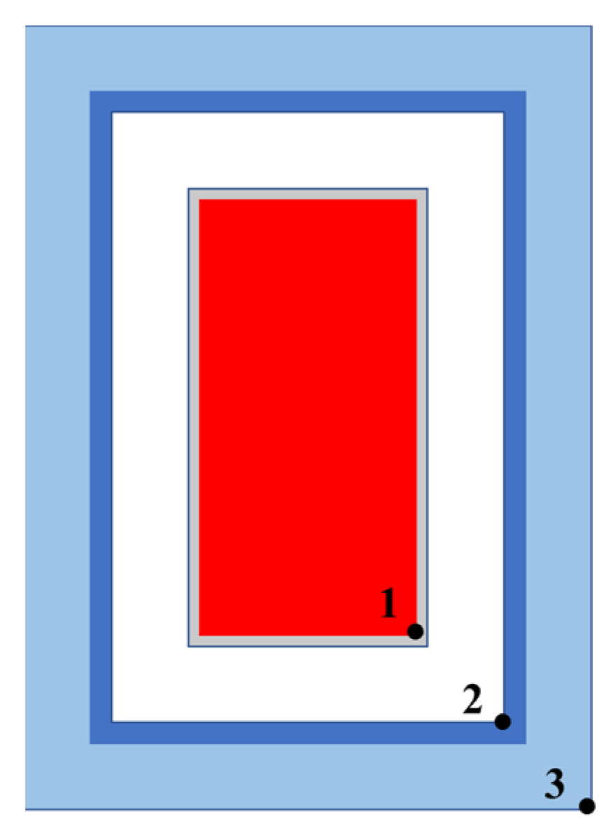
3.1. Complex Structure with Explosives

A complex structure with explosives is usually a system composed of different materials and components. It mainly includes three parts: multilayer solids, an air interlayer, and explosives. Figure 2 shows the physical model of the complex explosive structure used in this study.

Figure 2. Physical model of a complex explosive structure.

As shown in Figure 2, a complex structure with explosives contains five layers, in the order of a carbon-phenolic layer, TC11 titanium alloy layer, thick air interlayer, 304 stainless steel shell, and the PBX-9503 explosive. The thermal conductivities and the size of each component used in the numerical simulation are shown in Table 1.

Table 1. Thermal conductivities and thicknesses of the materials in each layer.

Material	Thickness/mm	Thermal Conductivity/(W/m·K)
Carbon-phenolic	30	0.48
TC11	10	7.5
Air	35	0.038
304 stainless steel	5	19.5
PBX-9503	$\varphi 100\times 200$	0.302

PBX-9503 explosive is a high-energy explosive that delivers the best comprehensive performance. The explosive has the advantages of high energy density, excellent detonation performance, and mechanical properties. The process of thermal decomposition is a nonlinear process, which can be expressed by the Arrhenius zero-order reaction:

$$s=\rho QZ{e}^{\left(-{\displaystyle \frac{E}{RT}}\right)}$$

(15)

where $\rho$ is the explosive density $({\mathrm{kg}/\mathrm{m}}^3)$, $Q$ is the reaction heat $(\mathrm{J}/\mathrm{kg})$, Z is the pre-factor $(1/\mathrm{s})$, $E$ is the reaction energy $(\mathrm{J}/\mathrm{mol})$, and $R$ is the ideal gas constant $(\mathrm{J}/(\mathrm{mol}\cdot \mathrm{K}))$. The parameter values of the PBX-9503 explosive are shown in Table 2.

Table 2. The specific related parameters of the PBX-9503 explosive [44].

Parameter	Value
$\rho$	$1845{\mathrm{kg}/\mathrm{m}}^3$
$Q$	4.78 × 105 $\mathrm{J}/\mathrm{kg}$
$Z$	4780/s
$E$	$143,900\mathrm{J}/\mathrm{mol}$
$R$	$8.314\mathrm{J}/(\mathrm{mol}\cdot \mathrm{K})$

3.2. Non-Periodic Thermal Boundary

The non-periodic thermal boundary concept is widespread in various scientific and engineering disciplines. In order to reveal the influence of non-periodic thermal boundary conditions on a thermal field, the flame boundary model is selected in this work. The pool of fire is the most effective scenario for modeling a flame boundary. The large eddy simulation has been applied for the flame simulation and gradient diffusion is the turbulence model used to close the scalar flux and the SGS momentum terms in the large eddy simulation. Radiation is introduced into the energy equation via the source terms, based on the Stefan–Boltzmann law. In our method, the time step is dynamically determined by an automated algorithm to simultaneously satisfy the Courant–Friedrichs–Lewy (CFL) condition governing convective stability and the Fourier number criterion for diffusive processes.

Therefore, the flame boundary and the complex structure with explosives are coupled. Figure 3a shows the coupled model and the structure with explosives is completely surrounded by the pool fire. Eight temperature measurement points are arranged in the model to track the gas phase temperature of the flame, as shown in Figure 3b.

Figure 3. The coupled model and the locations of the measurement points: (a) the model’s structure, surrounded by the pool of fire; (b) the specific locations of the flame gas phase temperature measurement points are shown in points 1–8.

The temperature of the coupled model in the pool of fire for the first 500 s is calculated, and the flame gas phase temperature of each measurement point is obtained. Figure 4 shows a graph of the temperature over time.

Figure 4. The temperature of each measurement point with time.

The results show that the flame temperature on the same surface of the structure is consistent; there is a great difference in the flame temperature on different surfaces, such as when, after 300 s, the temperature of measurement point 4 is 350 K higher than that of measurement point 6.

The reason for this difference in temperature on the various surfaces is the different combinations of fuel steam and oxygen. Measurement points 4 and 5 are located on the side of the structure (side surface) where the fuel steam and oxygen supply are sufficient. Full combustion leads to high temperatures. Measurement points 6, 7, and 8 are located on the upper surface of the structure (rear fire surface), and are not directly reached by the flames; therefore, the temperature is low. Measurement points 1, 2, and 3 are located on the lower surface of the structure (facing-fire surface), which are directly in contact with the flame. The combustion on the facing-fire surface is insufficient due to an inadequate oxygen supply, meaning that the temperature of the facing-fire surface is between the rear fire surface and the side surface.

According to the above conclusions, the pulsating flame temperatures measured on the different surfaces can be assigned to the structure. Then, the simulation of heat transfer between the flame and the wall and the simulation of heat transfer inside the complex structure with explosives can be conducted. The heat transfer model of the structure boundary is shown in Figure 5, which is mainly divided into two parts: the thermal radiation ${\dot{q}}_r^{″}$ of the high-temperature flame and the heat convection ${\dot{q}}_c^{″}$ of combustion.

Figure 5. Heat transfer mode between the flame and the wall.

Therefore, the formula for calculating the total heat flux ${\dot{q}}^{″}$ is:

$${\dot{q}}^{″}={\dot{q}}_c^{″}+{\dot{q}}_{″}^r=h(T_g-T_w)+\sigma F({\epsilon }_g{T}_g^4-{\epsilon }_w{T}_w^4)$$

(16)

where $T_g$ represents the gas phase temperature of the flame, $T_w$ represents the temperature of the outer wall of the structure, $h$ is the convective heat transfer coefficient, $\sigma$ is the Steffen-Boltzmann constant, $F$ is the angle of view coefficient, and ${\epsilon }_g$ and ${\epsilon }_w$ are the emissivity of the flame flue gas and the wall of the structure, respectively.

4. Results and Discussions

Based on the coupled model of a structure with explosives under flame boundary conditions, we carried out thermal field analysis and conducted rapid prediction. The POD-FVM reduced-order extrapolation method was employed and the influence of different POD modes on the results was analyzed.

4.1. Selection of POD Mode

The POD mode is critical to ensure accurate extrapolation. A snapshot was selected at 1-second intervals and a total of 500 snapshots were selected, based on the FVM numerical solution, and assembled into the temperature snapshot matrix in the following form:

$$T={\left[\begin{array}{cccc}{T}_1^1& T_1^2& \cdots & T_1^n\\ T_2^1& T_2^2& \cdots & T_2^n\\ ⋮& ⋮& ⋮& ⋮\\ T_m^1& T_m^2& \cdots & T_m^n\end{array}\right]}_{m\times n}$$

(17)

where m is the number of units and n is the number of snapshots.

Then the matrix (17) was decomposed and a total of 500 POD modes and their eigenvalues were obtained. The POD modes can be arranged according to the energy determined by the eigenvalues. The percentage of energy of each POD mode can be calculated according to the following formula:

$$I(i)={\displaystyle \frac{{\pi }_i}{{\displaystyle \sum _{i=1}^M{\pi }_i}}}\times 100\%$$

(18)

Figure 6 shows the energy ratio of the first 20 POD modes and the accumulated energy ratio of the reserved POD modes. It is evident that the first mode occupies the dominant energy ratio, reaching 86%, while the energy ratio tends to be 0 after the fifth mode. The accumulated energy of the first six modes has reached 99%, which basically reflects the main characteristics of the original temperature field.

Figure 6. The energy ratio of the first 20 modes and the accumulated mode energy ratio.

Figure 7 shows the 500th second normalization temperature of the structure, extracted from the first six POD modes. It can be seen that the first mode, which occupies the main energy, basically reflects the temperature field trend. Low-order modes with less energy constantly modify the boundary and the overall temperature field value within a small range.

Figure 7. The first six POD modes of the 500th second temperature field.

The amount of POD modes to be retained is calculated by setting the accumulated energy $\gamma$ according to Equation (6). Table 3 shows the number of POD modes that should be retained for the different accumulated energy values of $\gamma$ and the energy ratio of each mode set.

Table 3. Selection of the POD mode set.

Mode Set	γ Value	Number of POD Modes	Energy Ratio
1	99%	6	99.2004%
2	99.9%	13	99.9029%
3	99.99%	26	99.9906%
4	99.999%	55	99.9990%

The different POD mode sets are brought into the POD-FVM reduced-order extrapolation method to predict the thermal field. In the following sections, the accuracy and calculation cost of the reduced-order extrapolation method will be analyzed.

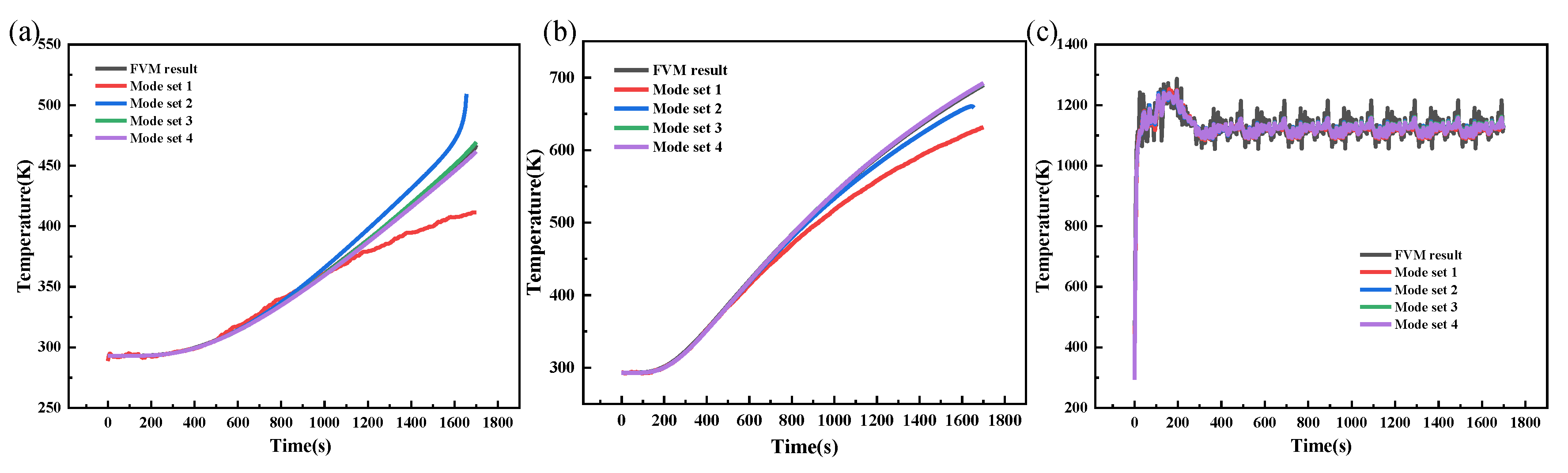
4.2. Accuracy Analysis of POD-FVM Reduced-Order Extrapolation

The key thermal indicators of a structure with explosives are temperature and explosion time. Figure 8 shows the temperatures of the cut surface of different mode sets after 1500 s. Except for the Z positions of 5 mm and 355 mm for mode set 1, the other mode sets have similar temperatures to the FVM result and show good agreement across all the cuts. This is due to the inability to capture slight energy thermal field trends in the case of low mode sets. As a result, the high-temperature areas are additionally highlighted. The deviation is gradually eliminated as the number of mode sets increases. From the temperature of the cut surfaces, the comprehensiveness of the thermal field in the extrapolation results of the algorithm can be demonstrated.

Figure 8. Temperature of the cut surfaces with different mode sets after 1500 s.

By harnessing the POD-FVM reduced-order extrapolation method, the precise moment of detonation is swiftly forecast. Mode sets 2, 3, and 4 accurately predict the explosion time, whereas mode set 1 does not. Figure 9 compares the explosion time predicted by the reduced-order method with the experimental data and delineates the relative errors for the various mode sets. Among the four mode sets, mode set 3 achieves the lowest relative error at 3.46%, with the maximum error remaining below 10%. This evidence supports the conclusion that the reduced-order model accurately predicts the explosion time. Moreover, the analysis indicates that the limited number of snapshots hinders the method’s ability to accurately capture the strong nonlinear heat transfer processes inherent in the explosion. This insufficiency results in the excessive smoothing of localized hot spots within the explosive material, ultimately causing mode sets that incorporate more modes to predict a delayed explosion time.

Figure 9. Comparison of the explosion times of different mode sets. The graph in the upper left corner shows the temperature cloud at the moment of the explosion; the colors are only indicative of the temperature.

The analysis in Section 3.2 and the simulated explosion time results show that the temperature change on the facing-fire surface of the structure is much more drastic. Specifically, the temperature change at the junction of the facing-fire surface and the side of the structure is critical and will reflect the detonation point of the explosive. Therefore, in order to further analyze the temperature field in each layer of the structure, three representative points are selected. Figure 10 shows the location of these three points.

Figure 10. The representative points made in the structure with explosives as shown in points 1–3.

Figure 11 shows the temperatures of three representative points predicted by the POD under each mode set, calculated by FVM. The temperatures are calculated for the first 1700 s.

Figure 11. The temperature of different points under each mode set in comparison with the FVM result: (a) temperature at point 1, (b) temperature at point 2, and (c) temperature at point 3.

It is evident that the temperature predictions at points 1 and 2 are successfully captured by four POD mode sets, and the temperature pulsation characteristics at point 3 are also successfully captured. Each layer of the structure with explosives achieves thermal protection and the temperature decreases from the outside to the inside.

In order to quantitatively examine the influence of different mode sets on the prediction results, the relative error formula is used to calculate the error of each point versus time:

$${\delta }_e={\displaystyle \frac{\left|T_{POD}-T_{FVM}\right|}{T_{FVM}}}\times 100\%$$

(19)

where $T_{POD}$ represents the temperature obtained by the POD of each POD mode set, and $T_{FVM}$ represents the temperature obtained by the FVM standard solution.

Figure 12 shows the relative error curves of each point with Equation (19). The results reveal that the relative error of mode set 1 and mode set 2 are larger than for mode set 3 and mode set 4 at point 1 and point 2. Notably, the errors accumulated gradually increase with time. The maximum relative errors of mode set 1 and mode set 2 reach 11.84% and 11.53%, respectively, at point 1. At point 2, the values drop to 8.46% and 3.43%. Moreover, there is a huge shift in the upward trend of the error of mode set 1 and mode set 2, rising at point 1 and point 2 when the time exceeds a time point. For example, the error of mode set 1 at point 1 shows a steep rise after 1000 s. However, at point 3, all four mode sets show good prediction ability, except in the early stages, where the relative error reaches 19.7%. A comparison study of the temperature data in Figure 11 reveals that this is due to the error introduced by the nature of the POD algorithm, namely, that the POD algorithm captures the main trends.

Figure 12. Relative error of different points under each mode set: (a) point 1, (b) point 2, and (c) point 3.

Moreover, the relative error of mode set 3 and mode set 4 with more POD modes is smaller than for mode set 1 and mode set 2 at each point. The maximum relative error of the three points is less than 5%. Thus, increasing the number of modes can compensate for the inherent shortcomings of the POD algorithm. However, this is accompanied by an increase in computational cost, which we will demonstrate in more detail in the next section.

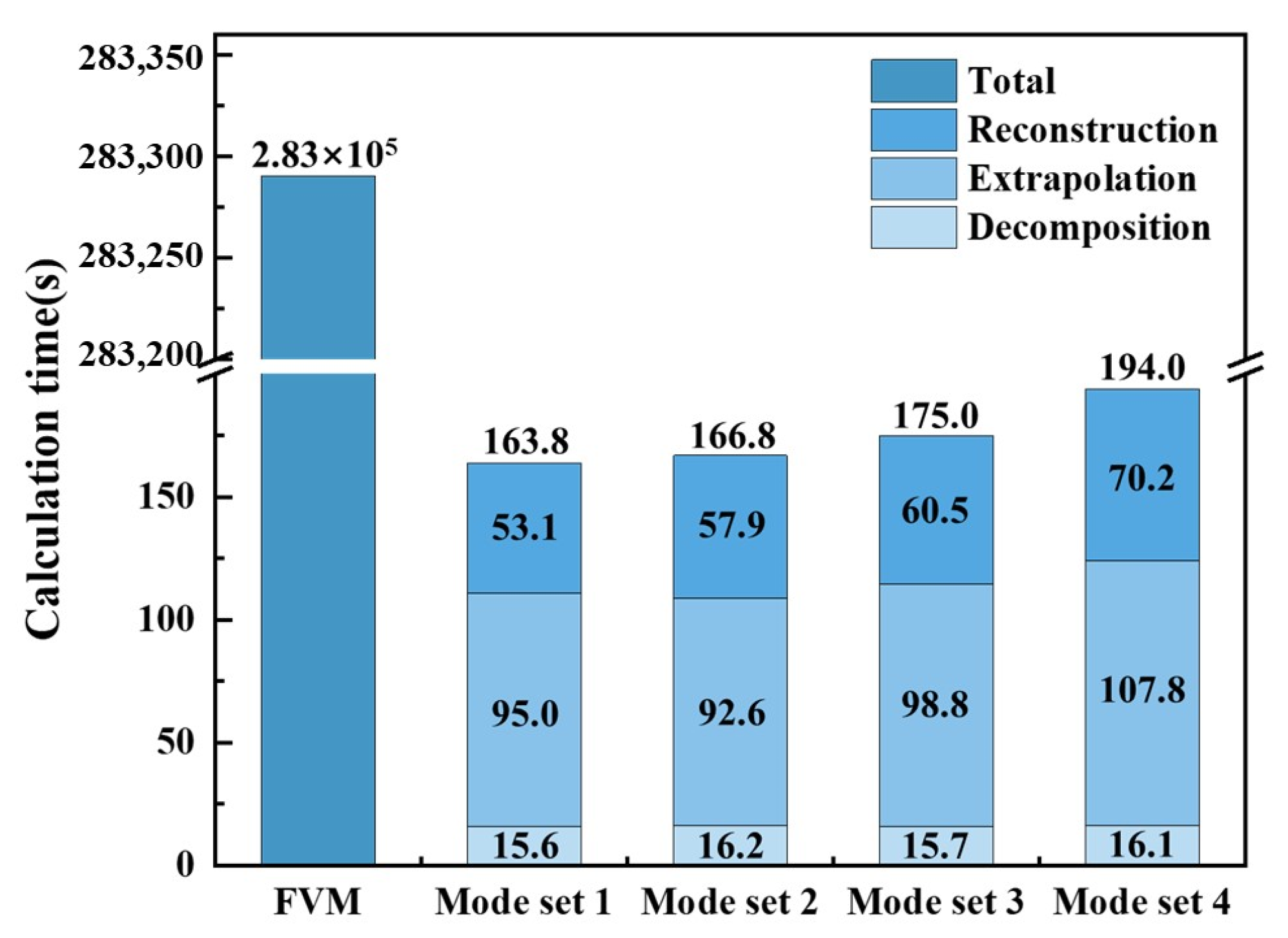
4.3. Computational Cost of the FVM and POD-FVM Reduced-Order Extrapolation Method

There is a consensus that the remarkable advantage of the POD order-reduction method is its fast calculation speed because of the great reduction of the degree of freedom of the algebraic equations system. Figure 13 shows the degree of freedom of each POD mode set. Mode set 1 reduces the number of degrees of freedom of each time-step algebraic equations system from 830,995 to 6 compared with the FVM method, achieving cross-order reductions. Although there is a slight increase in the degrees of freedom as the number of modes increases, a significant reduction is achieved compared to the traditional FVM method, as shown in Figure 13.

Figure 13. Comparison of the degrees of freedom of different methods.

The degree of freedom of the system of algebraic equations determines the calculation speed. Figure 14 shows the total time for calculating 1500 time steps by FVM and the reduced-order method for each mode set. The POD reduced-order time is divided into three parts: the POD decomposition time of the temperature snapshot matrix (decomposition), the time of mode coefficient extrapolation (extrapolation), and the time of reconstruction of the future temperature field (reconstruction).

Figure 14. Comparison of the calculation time of 1500 steps using different methods.

Compared with the calculation time for the FVM with the POD, it can be seen that the total calculation time of 1500 time steps after POD reduction is less than 200 s for each mode set, which is about 1400 times faster than the 2.83 × 10⁵ s needed with the FVM method. If the time taken to obtain the snapshot matrix is also included in the calculation time taken with the POD-FVM method, the calculation time needs to be added to another 9.43 × 10⁴ s. As a result, this is still a 76.6% improvement over the FVM method. The calculation speed has been greatly improved, highlighting the superiority of the POD-FVM reduced-order extrapolation method.

By comparing the calculation times of the four mode sets, the mode set with the greater degree of freedom takes longer to finish the calculations. The decomposition time is around the same for each mode set because of using the same temperature snapshot matrix. The extrapolation time and reconstruction time were affected by the degree of freedom. Thus, the calculation time shows a pattern of increasing with the increase in the degree of freedom.

5. Conclusions

We have developed a traditional proper orthogonal decomposition method, based on which, further extrapolation calculations were achieved by combining this with the FVM method. The temperature field of a complex three-dimensional structure can be predicted quickly and accurately. To validate the performance of the proposed algorithm, the multilayer thermally unstable structure and pulsating flame boundary conditions were selected and tested. Working according to the theory of accumulated energy, four mode sets were applied to conduct the investigation. The selection of POD modes had a greater impact on the extrapolation results; a mode set composed of more POD modes can improve the accuracy of the extrapolation results, although it will increase the calculation time accordingly. However, the prediction of explosion time is not positively correlated with the number of modes. The results obtained by the proposed method show good agreement with the experimental data and the FVM results. The relative error will increase as the extrapolation time increases in the small number mode set. At the same time, regardless of the number of POD modes, the disadvantage that the POD only captures the main trend is obvious, and further optimization of the algorithm is needed. The POD-FVM reduced-order extrapolation method reduces the degrees of freedom of the system from a magnitude of 10⁵ to 10¹, which greatly improves the computational speed by more than 1400 times. Above all, fast thermal field analysis under non-periodic boundary conditions is achieved, and this may aid in solving critical challenges in the rapid reconstruction and prediction of the temperature fields of sophisticated components, thereby enabling monitoring, diagnosis, and protection.

References

1. Mignolet, M.P.; Przekop, A.; Rizzi, S.A.; Spottswood, S.M. A review of indirect/non-intrusive reduced order modeling of nonlinear geometric structures. J. Sound Vib. 2013, 332, 2437–2460. [Google Scholar]
2. Luo, X.B.; Hu, R.; Liu, S.; Wang, K. Heat and fluid flow in high-power LED packaging and applications. Prog. Energy Combust. Sci. 2016, 56, 1–32. [Google Scholar]
3. Xing, G.Y.; Xue, S.; Han, J.C.; Zuo, H.Y.; Hu, R.; Tu, Z.K.; Luo, X.B. Turbulent lubrication model for journal-axial coupled hydrodynamic bearings without grooves. Tribol. Int. 2023, 190, 109036. [Google Scholar]
4. Xiang, L.Y.; Yu, X.J.; Hong, T.; Yang, X.; Xie, B.; Hu, R.; Luo, X.B. Performance of spray cooling with vertical surface orientation: An experimental investigation. Appl. Therm. Eng. 2023, 219, 119434. [Google Scholar]
5. Khandekar, S.; Sahu, G.; Muralidhar, K.; Gatapova, E.Y.; Kabov, O.A.; Hu, R.; Luo, X.B.; Zhao, L. Cooling of high-power LEDs by liquid sprays: Challenges and prospects. Appl. Therm. Eng. 2021, 184, 115640. [Google Scholar]
6. Xiang, L.Y.; Hu, R. Liquid directional steering. Matter 2022, 5, 13–15. [Google Scholar] [CrossRef]
7. Samadiani, E.; Joshi, Y. Multi-parameter model reduction in multi-scale convective systems. Int. J. Heat Mass Transf. 2010, 53, 2193–2205. [Google Scholar]
8. Xiang, L.Y.; Cheng, Y.H.; Yu, X.J.; Fan, Y.W.; Yang, X.; Zhang, X.F.; Xie, B.; Luo, X.B. High-performance thermal management system for high-power LEDs based on double-nozzle spray cooling. Appl. Therm. Eng. 2023, 231, 121005. [Google Scholar] [CrossRef]
9. Ostoich, C.M.; Bodony, D.J.; Geubelle, P.H. Fluid-thermal response of spherical dome under a Mach 6.59 laminar boundary layer. AIAA J. 2012, 50, 2791–2808. [Google Scholar]
10. Wang, Y.; Yu, B.; Cao, Z.Z.; Zou, W.Z.; Yu, G.J. A comparative study of POD interpolation and POD projection methods for fast and accurate prediction of heat transfer problems. Int. J. Heat Mass Transf. 2012, 55, 4827–4836. [Google Scholar]
11. Lu, K.; Zhang, K.Y.; Zhang, H.P.; Gu, X.H.; Jin, Y.L.; Zhao, S.B.; Fu, C.; Yang, Y.F. A review of model order reduction methods for large-scale structure systems. Shock Vib. 2021, 2021, 6631180. [Google Scholar] [CrossRef]
12. Lohrasbi, S.; Hammer, R.; Eßl, W.; Reiss, G.; Defregger, S.; Sanz, W. A modification to extended proper orthogonal decomposition-based correlation analysis: The spatial consideration. Int. J. Heat Mass Transf. 2021, 175, 121065. [Google Scholar]
13. Alonso, D.; Velazquez, A.; Vega, J.M. Robust reduced order modeling of heat transfer in a back step flow. Int. J. Heat Mass Transf. 2009, 52, 1149–1157. [Google Scholar] [CrossRef]
14. Pearson, K. LIII. On lines and planes of closest fit to systems of points in space. Philos. Mag. 1901, 2, 559–572. [Google Scholar] [CrossRef]
15. Benner, P.; Gugercin, S.; Willcox, K. A survey of projection-based model reduction methods for parametric dynamical systems. SIAM Rev. 1988, 57, 483–531. [Google Scholar] [CrossRef]
16. Nikolaidis, M.-A.; Ioannou, P.J.; Farrell, B.F.; Lozano-Durán, A. POD-based study of turbulent plane Poiseuille flow: Comparing structure and dynamics between quasi-linear simulations and DNS. J. Fluid Mech. 2023, 962, A16. [Google Scholar]
17. Wang, L.; Pan, C.; Wang, J.; Gao, Q. Statistical signatures of u component wall-attached eddies in proper orthogonal decomposition modes of a turbulent boundary layer. J. Fluid Mech. 2022, 944, A26. [Google Scholar] [CrossRef]
18. Lumley, J.L. The structure of inhomogeneous turbulent flows. In Atmospheric Turbulence and Radio Wave Propagation; Nauka: Moscow, Russia, 1967; pp. 166–178. [Google Scholar]
19. Sirovich, L. Turbulence and the Dynamics of Coherent Structures Part II: Symmetries and Transformations. Q. Appl. Math. 1987, 45, 573–582. [Google Scholar]
20. Hazenberg, M.; Astrid, P.; Weiland, S. Low order modeling and optimal control design of a heated plate. In Proceedings of the 2003 European Control Conference, Cambridge, UK, 1–4 September 2003; pp. 1240–1245. [Google Scholar]
21. Raghupathy, A.P.; Ghia, U.; Ghia, K.; Maltz, W. Boundary-condition-independent reduced-order modeling of complex 2D objects by POD-Galerkin methodology. In Proceedings of the 2009 25th Annual IEEE Semiconductor Thermal Measurement and Management Symposium, San Jose, CA, USA, 15–19 March 2009; pp. 208–215. [Google Scholar]
22. Georgaka, S.; Stabile, G.; Rozza, G.; Bluck, M.J. Parametric POD-Galerkin model order reduction for unsteady-state heat transfer problems. Commun. Comput. Phys. 2019, 27, 1–32. [Google Scholar] [CrossRef]
23. Hu, H.M.; Du, X.Z.; Yang, L.J.; Yang, Y.P.; Cheng, T.R. Cross scale simulation on transport phenomena of direct air-cooling system of power generating units based on reduced order modeling. Int. J. Heat Mass Transf. 2014, 75, 156–164. [Google Scholar]
24. He, S.P.; Wang, M.J.; Zhang, J.; Tian, W.X.; Qiu, S.Z.; Su, G.H. A deep-learning reduced-order model for thermal hydraulic characteristics rapid estimation of steam generators. Int. J. Heat Mass Transf. 2022, 198, 123424. [Google Scholar]
25. Han, D.X.; Yu, B.; Yu, G.J.; Zhao, Y.; Zhang, W.H. Study on a BFC-based POD-Galerkin ROM for the steady-state heat transfer problem. Int. J. Heat Mass Transf. 2014, 69, 1–5. [Google Scholar] [CrossRef]
26. Jiang, W.W.; Pan, T.; Jiang, G.H.; Sun, Z.Y.; Liu, H.Y.; Zhou, Z.Y.; Ruan, B.; Yang, K.; Gao, X.W. Data-driven physical fields reconstruction of supercritical-pressure flow in regenerative cooling channel using POD-AE reduced-order model. Int. J. Heat Mass Transf. 2023, 217, 124699. [Google Scholar] [CrossRef]
27. Luo, Z.D.; Li, H.; Sun, P.; An, J.; Navon, I.M. A reduced-order finite volume element formulation based on POD method and numerical simulation for two-dimensional solute transport problems. Math. Comput. Simulat. 2012, 42, 1263–1280. [Google Scholar] [CrossRef]
28. Luo, Z.D.; Li, H.; Sun, P.; Gao, J.Q. A reduced-order finite difference extrapolation algorithm based on POD technique for the non-stationary Navier–Stokes equations. Appl. Math. Model. 2013, 37, 5464–5473. [Google Scholar]
29. Luo, Z.D.; Nie, S.; Li, H. A reduced order extrapolated difference algorithm for parabolic equations based on POD method. Math. Pract. Cogn. 2013, 43, 161–167. [Google Scholar]
30. Vuppula, V.K.R.; Ramanujam, M.; Runkana, V. Reduced-order modeling of conjugate heat transfer in lithium-ion batteries. Int. J. Heat Mass Transf. 2024, 227, 125537. [Google Scholar] [CrossRef]
31. Teng, F.; Luo, Z.D.; Yang, J. A reduced-order extrapolated natural boundary element method based on POD for the parabolic equation in the 2D unbounded domain. Comput. Appl. Math. 2019, 38, 102. [Google Scholar]
32. Frey, P.J.; George, P.L. Mesh Generation Application to Finite Elements, 2nd ed.; ISTE Ltd.: London, UK; John Wiley & Sons Publishing: Indianapolis, IN, USA, 2008. [Google Scholar]
33. Wu, S.; Li, M.H.; Zhang, Z.L. Thermal protection design and analysis of complex explosive structures in fire environment. Acta Ordnance Eng. 2014, 35, 1275–1280. [Google Scholar]
34. Jiang, C.Y.; Soh, Y.C.; Li, H. Two-stage indoor physical field reconstruction from sparse sensor observations. Energy Build. 2017, 151, 548–563. [Google Scholar]
35. Azzouz, M.S.; Guo, X.; Przekop, A.; Mei, C. Comparison of PDE/Galerkin and FEM for nonlinear aerospace structures analyses. In Proceedings of the 44th Structures, Structural Dynamics and Materials Conference, Norfolk, VA, USA, 7–10 April 2003. [Google Scholar]
36. Xing, G.Y.; Xue, S.; Hong, T.; Zuo, H.Y.; Luo, X.B. A Novel Hydrodynamic Suspension Micropump Using Centrifugal Pressurization and the Wedge Effect. Sci. China Technol. Sci. 2023, 66, 2047–2058. [Google Scholar]
37. Carere, G.; Strazzullo, M.; Ballarin, F.; Rozza, G.; Stevenson, R. A weighted POD-reduction approach for parametrized PDE-constrained optimal control problems with random inputs and applications to environmental sciences. Comput. Math. Appl. 2021, 102, 261–276. [Google Scholar]
38. Yang, X.; Zhang, X.F.; Zhang, T.X.; Xiang, L.Y.; Xie, B.; Luo, X.B. Paving continuous heat dissipation pathways for quantum dots in polymer with orange-inspired radially aligned UHMWPE fibers. Opto-Electron. Adv. 2024, 7, 240036. [Google Scholar]
39. Li, T.Y.; Gao, Y.Q.; Han, D.X.; Yang, F.S.; Yu, B. A novel POD reduced-order model based on EDFM for steady-state and transient heat transfer in fractured geothermal reservoir. Int. J. Heat Mass Transf. 2020, 146, 118783. [Google Scholar]
40. Souza, Y.P.; Loureiro, F.S.; Mansur, W.J.; Ferreira, W.G.; Camargo, R.S. A time-domain POD approach based on numerical implicit and explicit Green’s functions for 3D elastodynamic analysis. Comput. Struct. 2023, 275, 106921. [Google Scholar]
41. Zhang, X.; Xiang, H. A fast meshless method based on proper orthogonal decomposition for the transient heat conduction problems. Int. J. Heat Mass Transf. 2015, 84, 729–739. [Google Scholar]
42. Zhu, Q.H.; Liang, Y.; Gao, X.W. A proper orthogonal decomposition analysis method for transient nonlinear heat conduction problems. Part 1 Basic Algorithm. Numer. Heat Transf. Part B Fundam. 2019, 77, 87–115. [Google Scholar]
43. Moukalled, F.; Mangani, L.; Darwish, M. The Finite Volume Method in Computational Fluid Dynamics; Springer International Publishing: Cham, Switzerland, 2016. [Google Scholar]
44. Wu, S.; Li, M.H.; Zhang, Z.L. Numerical Simulation of Heat Transfer Problems in Structure with Explosive under Fire. Chin. J. Energ. Mater. 2014, 22, 617–623. [Google Scholar]