Data-Driven Pavement Performance: Machine Learning-Based Predictive Models

Featured Application

This research provides effective methodology for pavement performance predictions using the data obtained from finite element analysis and merging it with machine learning algorithms.

Abstract

Traditional methods for predicting pavement performance rely on complex finite element modelling and empirical equations, which are computationally expensive and time-consuming. However, machine learning models offer a time-efficient solution for predicting pavement performance. This study utilizes a range of machine learning algorithms, including linear regression, decision tree, random forest, gradient boosting, K-nearest neighbour, Support Vector Regression, LightGBM and CatBoost, to analyse their effectiveness in predicting pavement performance. The input variables include axle load, truck load, traffic speed, lateral wander modes, asphalt layer thickness, traffic lane width and tire types, while the output variables consist of number of passes to fatigue damage, number of passes to rutting damage, fatigue life reduction in number of years and rut depth at 1.3 million passes. A k-fold cross-validation technique was employed to optimize hyperparameters. Results indicate that LightGBM and CatBoost outperform other models, achieving the lowest mean squared error and highest R² values. In contrast, linear regression and KNN demonstrated the lowest performance, with MSE values up to 188% higher than CatBoost. This study concludes that integrating machine learning with finite element analysis provides further improvements in pavement performance predictions.

1. Introduction

Machine learning models can be used to predict pavement performance in terms of rutting and fatigue cracking. The use of autonomous trucks in this research further includes the aspects of different later wander modes, lane width variations that are directly linked to the behaviour of autonomous trucks. Autonomous trucks are bound to bring new challenges to current the transport infrastructure system, specifically on the impact of autonomous trucks on pavements. Autonomous trucks can be programmed by the manufacturers to a controlled lateral path within the highway lane. It has been proposed to use the zero lateral wander to improve traffic efficiency and safety [1]. However, this type of lateral wander has detrimental implications on the pavement. An alternative option is to use uniform wander mode where the channelized loading from autonomous trucks can be minimized by uniformly distributing the lateral paths within the lane [2]. The performance of uniform wander mode can be further increased by adding the truck platooning function, which works in favour of increased fuel efficiency for autonomous trucks [3]. Machine learning is part of the artificial intelligence types used in performance prediction modelling of impacts on pavements. Traditional methods for performance evaluation of pavements require complicated calculations and procedures to analyse the data and results. With the provision of a vast variety of available data, predictions based on pavement material properties, traffic details and environmental details can be made. Therefore, the model structure is designed based on the quantitative relationship between input variables and output variables, thereby developing the machine learning model [4].

The concept of machine learning is used to analyse large data and performance predictions of future pavement performance parameters based on training the algorithm. Machine learning is trained through the examples generated through various iterations of data and developing the relationship between input and output variables [5]. The artificial neural network (ANN) is composed of several interconnected processing units present in layer forms (input layers, hidden layers, output layer). The ANN is composed of three different types, consisting of the recurrent neural network (RNN), convolutional neural network (CNN) and multi-layer perception neural network (MLPNN), with hidden layers greater than one being part of the deep neural network [6].

A variety of parameters related to autonomous trucks in terms of traffic speed, lateral wander options, tire types and axle configurations are taken into account. Furthermore, the aforementioned parameters are combined, and their effect on rutting and fatigue damage is evaluated using the data obtained from finite element modelling. The use of machine learning models for fatigue cracking and rutting progression of pavement based on numerous input parameters can significantly reduce the calculation time and quantity of data needed for analysis, since these models are fundamentally proficient for their role in pattern recognition, classification, data identification and predictions [7].

For fatigue cracking predictions, transfer functions are employed for alligator cracking and longitudinal cracking [8]. The term Stress Intensity Factor (SIF) has been used previously for performing cracking analysis of asphalt pavements [9]. Semi-analytical finite element modelling in conjunction with neural networks is performed for evaluating SIF. The neural network models are then trained to yield the SIF based on semi-analytical finite element modelling.

In the existing research, different machine learning models have not been optimized with the k-fold technique, and their prediction capability has not been measured with an extensive range of input and output variables. Moreover, the performance of each model is measured by comparing it with the relevant laboratory results for material behaviour. However, in this research, the mechanical behaviour of the pavement is evaluated by using finite element modelling; therefore, the parameters used are validated beforehand. Thus, in this research, the predictive performance using the finite element modelling is further reinforced by using the machine learning models which serves as a research gap in the current research.

This research provides an alternative option for predicting pavement performance in terms of rutting and fatigue cracking that has previously been predicted using finite element modelling. The addition of further prediction using machine learning models increases the prediction accuracy of the preexisting output variables. Therefore, in the previous research, only the prediction of certain pavement distress mechanisms has been performed directly using machine learning algorithms with a narrow range of input variables. Moreover, this research also integrates the autonomous trucks and their corresponding parameters including lane width variations, lateral wander modes and asphalt thickness variations into machine learning models. Therefore, a wide range of input variables associated with autonomous trucks are included, and evaluation of the prediction accuracy of different machine learning models is performed.

The novelty of this research consists of integrating the machine learning algorithms in predicting the performance indicators of flexible pavements in terms of rutting and fatigue cracking from the preexisting data consisting of input variables and already evaluated output variables. Since finite element modelling can be used to predict the performance of flexible pavements, the use of machine learning algorithms can be included to perform similar predictions but in a fraction of time. Therefore, the focus of this research is to evaluate the performance of different machine learning algorithms available, compare their performance in predictions and outline the best-performing algorithm.

2. Previous Research

Machine learning models including gradient boosting, Support Vector Regression (SVR), random forest, decision tree, linear regression, K-nearest neighbour, LightGBM and CatBoost have previously been used in various dominions of pavement engineering ranging from pavement design, construction, maintenance and pavement performance predictions.

2.1. General

Gong et al. [8] further enhanced the capability of transfer functions to predict the fatigue performance of asphalt pavement using a gradient boost model. R programming language was used to develop the model. The damage index based on traffic volume, subgrade modulus, layer thickness, traffic volume and climatic conditions were obtained. The results showed a significant performance of prediction using the gradient boost model, with error decreased to 4.35%. However, in this research, the damage index was taken into account without any distress mechanism including rutting and fatigue cracking, thereby requiring the use of distress mechanism evaluation in future research.

Wu et al. [9] used a random forest algorithm for optimization of input variables for improvement in prediction accuracy of rutting prediction artificial neural network models in the US and Canada. Variables taken into account were pavement structural properties, climatic conditions and traffic conditions. Results showed good capability of the proposed model to predict rut depth progression, with the coefficient of determination at 0.932 and root mean square error of 1.108 mm. However, in this research, the number of cycles to fatigue damage were not included in the scope; therefore, in the current research, the fatigue damage evaluation based on the input data is performed.

Haddad et al. [10] proposed a deep neural network model for rutting prediction of asphalt pavements with a minimum amount of input variables. The data for the deep neural network were extracted from a long-term pavement performance database. Performance of the DNN model was compared with that of the multivariate linear regression model. Results showed higher predictive performance of the model than conventional models. Furthermore, the proposed model could rank the input parameters based on their impact on rutting. However, in this research, the developed DNN did not incorporate the fundamentals of CatBoost and LightGBM for further optimizing the network’s performance; therefore, in the current research, the number of folds is evaluated for each model type to increase its predictive performance.

Chen et al. [11] developed neural network-based models for the prediction of rutting, skid resistance, transverse cracking and surface distress. Mean impact values were employed to analyse the impact of input variables on different damage mechanisms by developing five different models based on the neural network. Results showed good capability of neural network models for prediction of pavement damage conditions, with a coefficient of determination of 0.8692. Furthermore, it was found that pavement age and maintenance type have the highest impact on rutting regression in pavements.

Cheng et al. [12] developed an ANN with four layers to analyse the forecast leading to development of rutting based on the input variables from the data, including traffic volume, climatic conditions, pavement characteristics and maintenance conditions. The random forest decision tree algorithm was used to compute feature importance in order to analyse its importance with the target. The outputs of the model were rut depth, wheel track width and cross-sectional area. Results showed that rutting was also affected by the thickness of the surface layer and voids in the asphalt mixture. Results concluded with the development of rutting evaluation index for scaling the rutting severity. Although different machine learning algorithms have been used in previously conducted research, in this research, a wide range of machine learning algorithms have been compared in terms of rutting and fatigue cracking, and furthermore, the correlation analysis of input and output variables has been performed.

2.2. Support Vector Regression

Tran et al. [13] previously used SVR and multiple linear regression for performance prediction of freeways. Coefficient of determination (R²) and mean squared error (MSE) were used to analyse performance prediction of these models. Pavement distress mechanisms in term of rutting, roughness and fatigue cracking were analysed based on traffic and climate data. Results showed prediction performance for multiple linear regression and SVR by showing good prediction of rutting and roughness values.

Wang et al. [14] employed the use of SVR for predicting pavement performance from input parameters consisting of maximum and minimum temperature variations, rainfall and traffic volume. Data were collected by performing coring at different test sections of the pavement and collected for SVR. The data were then trained, and results showed high capability of the proposed model to predict pavement performance in terms of pavement temperature variations throughout the season.

2.3. Random Forest

Bajic et al. [15] employed the use of random forest algorithm and SVR for road roughness prediction. The analysis was performed on a 50 km stretch of road using the segment alignment procedure. Data in terms of car acceleration and variation in car speeds were used for the models. Models were trained to predict the exact values of IRI (International Roughness Index). Results showed good prediction capability of random forest algorithm and SVR with R² value of 0.66.

Gong et al. [16] used the random forest regression for prediction of IRI using input variables consisting of traffic, climate and distress measurements. A total of 11,000 samples of data were collected from the database of long-term pavement performance programs. Performance of random forest regression was compared with that of multiple linear regression. Results showed that random forest outperformed the multiple linear regression by yielding the R² of 0.95. Furthermore, it was found that fatigue cracking and rutting had the highest influence on IRI.

Gong et al. [8] employed the random forest algorithm for prediction of moisture damage in flexible pavements. Data were partitioned into smaller spaces by constructing the decision tree matrix. The training dataset was then input to fit the tree with further two hyperparameters. Factor importance was also analysed, and results showed that significant increase in rutting and deflection would lead to moisture damage in pavement. The proposed model could predict the moisture damage along with rutting performance with an error rate of 16.67%.

Yang et al. [17] used random forest models to predict pavement performance based on design life variations, base or subbase course with asphalt concrete, Portland cement concrete pavement with or without dowel bars. The pavement design program AASHTOWare was utilized for both flexible and rigid pavements for validating the performance prediction of the model. The random forest model was trained to predict pavement layer thickness, material properties, pavement distress and climate conditions by utilizing a total of 79,600 design scenarios. Results showed good prediction performance of random forest model for predicting the pavement distress and design layer thickness of AC and PCC pavements.

2.4. K-Nearest Neighbour

Fang et al. [18] used the K-nearest neighbour (KNN) on a multiple regression algorithm to find the missing data of sensors in bridge maintenance predictions. Spatial correlation from the neighbouring sensors was performed to increase the prediction accuracy of regression analysis. Furthermore, time correlation was also performed based on the time series data. Results showed good capability of the KNN multiple regression algorithm for predicting the missing sensor data.

Nguyen et al. [19] used the KNN among other algorithms including random forest with 107 data positions and 8 features to investigate the choice accuracy of the best machine learning model for predicting cracking tolerance index. Root mean square error combined with Monte Carlo simulation was used to check the accuracy of each model. Results showed that the percentage of aggregate passing 4.75 mm sieve had the highest effect on variation in cracking tolerance index with all models able to predict the tolerance index with good accuracy.

2.5. Linear Regression and Decision Tree

Wang et al. [20] incorporated AdaBoost to compare the prediction using linear regression approach of MPEDG for prediction of road roughness. Results showed that gradient boosting using AdaBoost significantly outperformed the prediction capabilities with reduced errors when compared to the linear regression approach.

Matei et al. [21] used the cloud decision tree to find the most appropriate rehabilitation scenario for pavements. A general decision-making model was developed based on various decision trees. Results show good capability of the proposed load-based decision tree model with an accuracy of 80%, with fatigue cracking and IRI being the most important parameters for decision-making in the pavement rehabilitation process. Pappalardo et al. [22] used the decision tree for analysing the performance of lane support systems in vehicles. The faults for the lane support system were detected in both day and nighttime conditions. Results showed good capability of the decision tree model to predict the fault related to the performance of lane support systems. Furthermore, it was found that faults would increase further with roads sections having less than 200 m of radius and inadequate visibility of road markings.

2.6. Gradient Boosting, LightGBM, CatBoost

Machado et al. [23] used the gradient boosting decision tree model with the gradient-based one-side sampling and exclusive feature bundling to further enhance the prediction capability of GBM. Approximation ratios for the developed LightGBM were compared against the XgBoost model, and results showed fast prediction of data among the same base line. Furthermore, LightGBM leads to 20 times increase in the training speed of the gradient boosting decision tree. Hu et al. [24] predicted the skid resistance using the LightGBM, Xgboost and SVR algorithms, and 3D point cloud data for the asphalt surface were used to train the algorithms based on the surface texture of asphalt pavements. The performance of each algorithm was evaluated based on the dataset and training. Results concluded with LightGBM exhibiting the highest accuracy with R² of 92.83%.

Guo et al. [25] used the ensemble learning model developed with LightGBM for roughness and rut depth predictions. Results were compared with that of ANN and showed good capability of the developed LightGBM to predict rut depth and IRI. Barua et al. [26] used the LightGBM for prediction of pavement condition index of airport pavements by comparing it with non-linear regression models, random forest models and artificial neural networks. Results showed good capability of the LightGBM to detect cracks using the imagery and outperforming the other models’ capability to predict with accuracy to real site conditions. Xiao et al. [27] used various versions of gradient boosting techniques including Adaptive Boosting (AdaBoost), LightGBM, gradient boosting decision tree (GBDT) and categorial boost (CatBoost) for faulting predictions in rigid pavements. The models were combined with the tree-structured Parzen simulator (TPE). Data were obtained from a long-term pavement performance database with over 160 observations. Results showed good capability of models to predict the faulting, with CatBoost being the most accurate with an R² value of 0.906. Historical data consisting of 17 variables with 160 instances of observations from a long-term pavement performance program (LTPP) were utilized. Results concluded with the CatBoost algorithm showing the highest accuracy with R² of 0.906. Furthermore, CatBoost was able to identify the primary affecting factors in terms of faulting.

3. Machine Learning Algorithms

3.1. Linear Regression

Linear regression has previously been used for analysing the correlation between the input and output variables. In linear regression, a relationship of a single dependent variable with one or more independent variables is established. A continuous response variable is defined by a linear function. Linear regression models are time-efficient and simplistic in terms of data processing and fitting the generated model to the dataset [28]. With the increase in the number of explanatory variables, multiple linear regression is used. The model’s prediction is maximized by weighting each explanatory variable using the regression analysis. Therefore, the target variables (rut depth at 1.3 million passes, number of passes to reach rut depth of 6 mm, reduction in fatigue life and number of passes to reach fatigue damage) are predicted based on various explanatory variables. The relationship between the dependent and independent variables is defined by the following Equation (1).

$$Y=C+a_1{X}_1+a_1{X}_1+\dots +a_n{X}_n$$

(1)

where $Y$ is the output variable, $C$ is the value of output varibale at $a_n=0$, $a_n$ are the regression coefficients and $X_n$ are the values of input variables.

3.2. Random Forest

Random forest is a tree-based algorithm that employs classification and regression trees for predicting and analysing the data. It is a group of decision trees that are created using the random sequence of input variables [15]. It classifies the random dataset into multiple branches at each stage, from the initial node to the terminal nodes. The random forest algorithm randomly selects the data from the dataset by constructing various decision trees, and prediction is performed by combining the results of this decision tree. It also employs the modified bragging method to increase the accuracy of predictions. A group of randomly developed decision trees is constructed, and predictions are made based on the mean regression of individual trees [16]. Partitioning of data into smaller groups is performed to train the trees. Random forest regression can also be used for improperly balanced data with missing parameters.

3.3. Support Vector Regression

SVR is based on statistical learning theory generated from data, which is an integral part of machine learning. It is a kernel model used for multiscale classification of tasks obtained from input datasets. In SVR, an optimum hyperplane is used to arrange the irregular data into multiple arranged classes [29]. In SVR, a prediction vector from the dataset is predicted by reestablishing a nonlinear relationship between the test data and the SVR. SVR also employs the use of the structural risk minimization principle [30]. SVR finds a hyperplane by dividing the features into various domains, and the hyperplane with the maximum space is termed an optimal hyperplane. It is used both for classification and regression analysis. In SVM, best fitting of hyper plane data is used to optimize the data arrangement by controlling an error to a specific range, which leads to minimization of large error [31]. SVM increases the margin boundary tolerance between each class, thereby leading to clear identification of the effect of each input variable (16). The non-linear function $f\left(x\right)$ is used to help fit the data. The hyperplane is identified using the following Equation (2).

$$f\left(x\right)={\omega }^{T}x+b$$

(2)

where $f\left(x\right)$ is the hyperplane, $x={\left\{x_i\right\}}_{i=1\dots N}$ are the features, $w={\left\{{xw}_i\right\}}_{i=1\dots N}$ are the vectors and $b=w_0$ is the bias.

3.4. K-Nearest Neighbour

K-nearest neighbour (KNN) is used for classifications and regression purposes, and it is identified as a non-parametric parametric machine learning algorithm; predictions are made by finding the K-nearest data points based on the input and making an average of target values [18]. Objects are classified by identifying the neighbours in data points with the provided sample units. The Euclidean distance is used to identify the distance between an object and its neighbours [32]. The nearest neighbour technique can be used both for univariate and multivariate predictions and can be used for a wide variety of datasets [33]. Since the KNN regression requires the calculation of distances between new and existing data points, it can be computationally expensive [34]. Furthermore, the quality of predictions is governed by taking the right value for K. Furthermore, KNN can be used to identify the missing values and can also be used for rutting performance characterization of asphalt pavements [4].

3.5. Gradient Boosting

Gradient boosting deals with a series of machine learning models dependent on decision trees. Boosting is conducted to improve the performance of a learning algorithm. A base or weak learner is applied to different weights of data points. Decision trees are used to fit gradients. LightGBM is another boosting model developed to perform operations in terms of finding missing values and higher computational speeds [25]. Different versions of gradient boosting include AdaBoost, gradient boosting decision tree (GBDT) and categorial boost (CatBoost). In gradient boosting, the residuals are estimated by first-order and second-order Taylor expansions of lost functions. A combination of multiple regression trees forms a tree group, and the predicted values of the group are then generated to compare them with the true values of the whole group to increase the accuracy [20].

3.6. Decision Tree

Decision tree-based algorithms are part of the machine learning approach and frequently used in data mining. In a decision tree, the data are split based on the most important feature that can affect the transition of data at a higher rate. Results continue to split until the data subset can be further divided. In the final process, any of the subsets with no correlation to the model are removed. Decision trees perform a hierarchical segmentation for different sets of units by identifying the rules and categorizing them into different classes and variables that might affect each unit. Therefore, the optimum decision rule is identified based on hierarchical segmentation [22]. A single explanatory variable at each step leads to the provision of the rule for a decision tree.

3.7. LightGBM

LightGBM is used for classification and regression of datasets. LightGBM is a part of a gradient boosting algorithm consisting of gradient-based one-side sampling (GOSS) and exclusive feature bundling (EFB) [23]. LightGBM works with residuals that are approximated, where Taylor expansions for first-order and second-order of loss functions are employed [24]. In LightGBM, multiple trees are grouped to form a tree group, and the predicted value of each tree group is made closer to the actual value for faster prediction performance. LightGBM consists of initializing the parameters and then defining the boundary value of each parameter. In LightGBM, samples are selected based on the gradient. For a higher gradient, it is based on percentage, and for a lower gradient, selection is based on random selection for a reduction in the number of samples [35].

3.8. CatBoost

Categorial boost (CatBoost) is a part of a gradient boosting decision tree algorithm, where the strategy for minimizing the loss function is utilized to increase the prediction accuracy. In CatBoost, the concept of symmetric tree arrangement is applied, where the symmetry between left and right decision trees is kept constant during iterations. In CatBoost, base predictors are employed in terms of binary decision trees. Furthermore, a binarization feature is used in CatBoost for encoding, and binary vectors are used to represent the indices of each leaf node [27]. In CatBoost, multiple categorial features and their combinations are combined into a current tree. Furthermore, the weak learner is further trained to reduce the gradient bias using ordered boosting [36].

4. Methodology

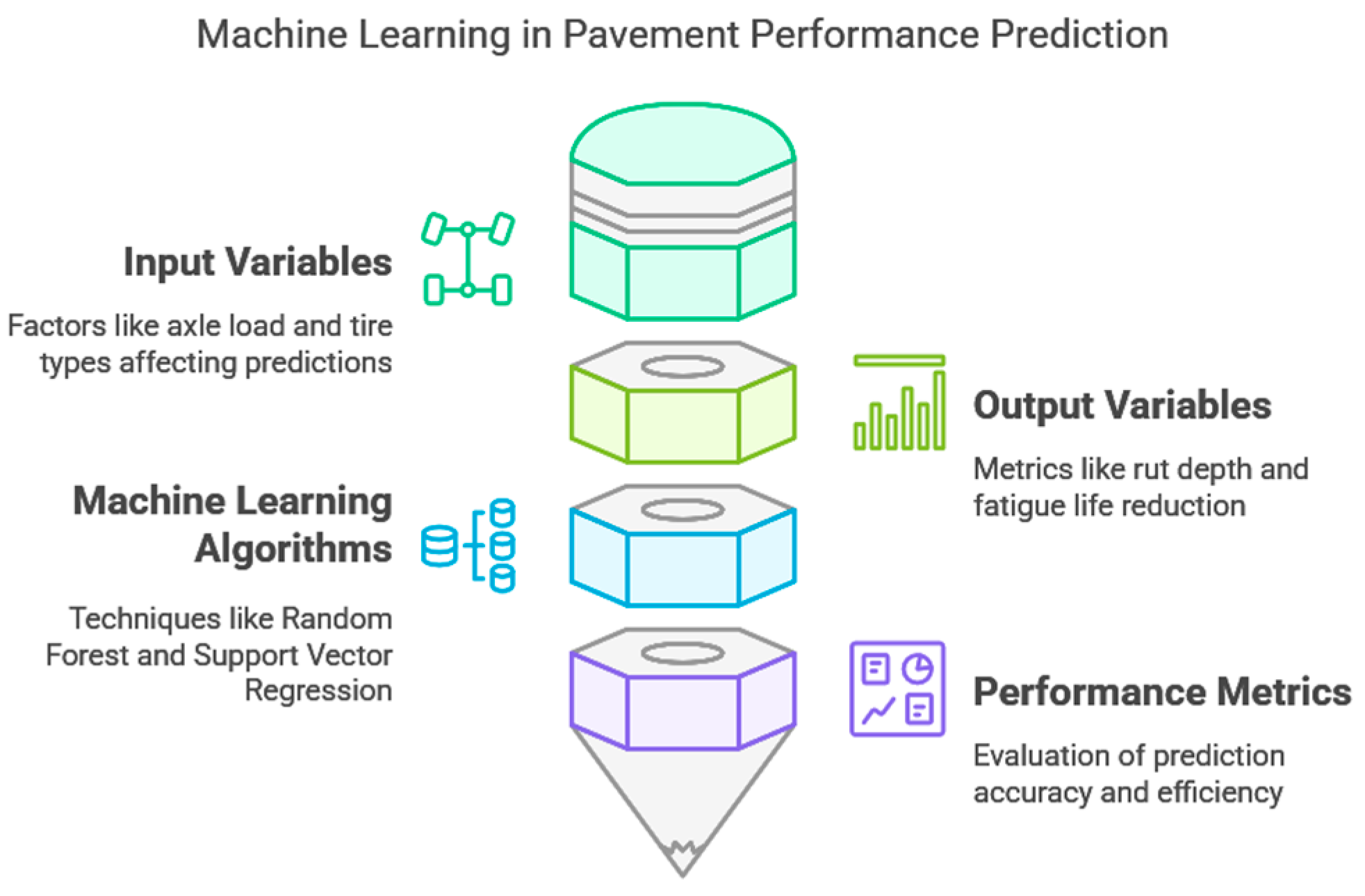
A total of 350 data points have been selected with input and output parameters. Input parameters include axle loading type, total truck load in GWT, lateral wander modes (Uniform and Zero wander), lane width variations (3.75 m and 4.2 m), asphalt layer thickness variations (16 cm and 20 cm) and tire footprint type (dual tire, single wide tire). Output parameters include fatigue life reduction in years, number of passes to fatigue damage, rut depth and number of passes to reach rut depth of 6 mm. For larger data, three forms of data treatment are used to achieve the optimized model for prediction against actual values. This includes training of 70% data, where the first remaining 15% of the data is validated and the last remaining 15% of the data is tested. A brief summary of this research is shown in Figure 1.

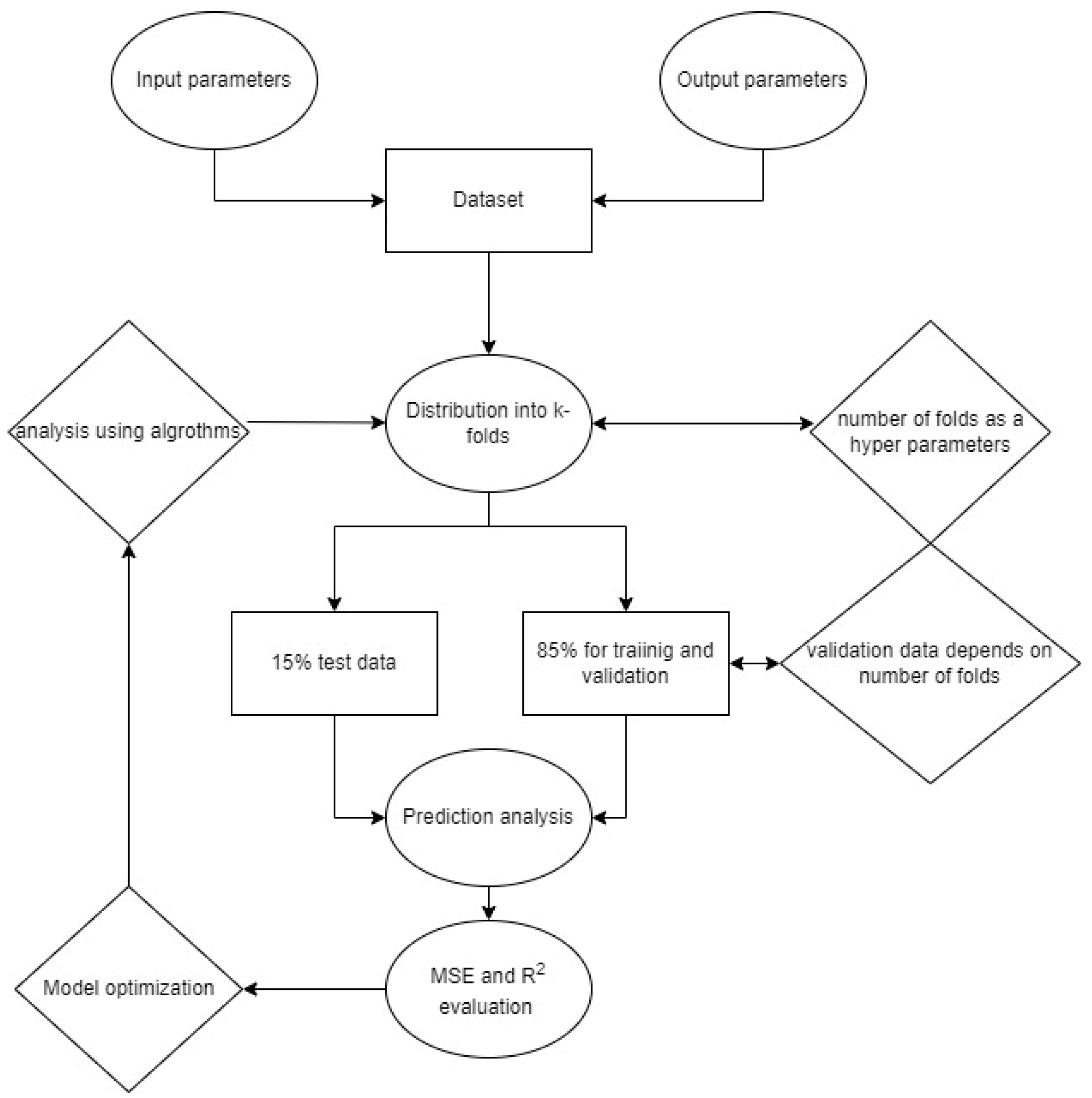
Since the quantity of data points is less and the actual data is validated, the k-fold cross-validation technique is used where the prediction of models is analysed by dividing the data into k subsets or folds. According to the type of algorithm (random forest, decision tree, gradient boosting, K-neighbour, SVR, LightGBM and CatBoost), the number of folds may vary based on the capability of these individual models to predict the results.

As observed from Figure 2, test data are kept at 15%, and the remaining 85% is kept for validation and training. The amount of data used for validation varies with the number of folds used for each algorithm tested. If there are nine folds for the decision tree algorithm, then 95% of the data is used for validation, and 5% is used for training. Furthermore, number of k-folds are used as a hyperparameter, and the optimum number of folds for each algorithm is evaluated based on the highest prediction strength of each model. Each algorithm possesses a different number of folds and corresponding MSE and R² values through iterations. The model is further optimized during prediction analysis where two different metrics are used to evaluate model performance including mean square error and R². The MSE values for each algorithm and their corresponding number of folds are averaged and shown in the Section 6.

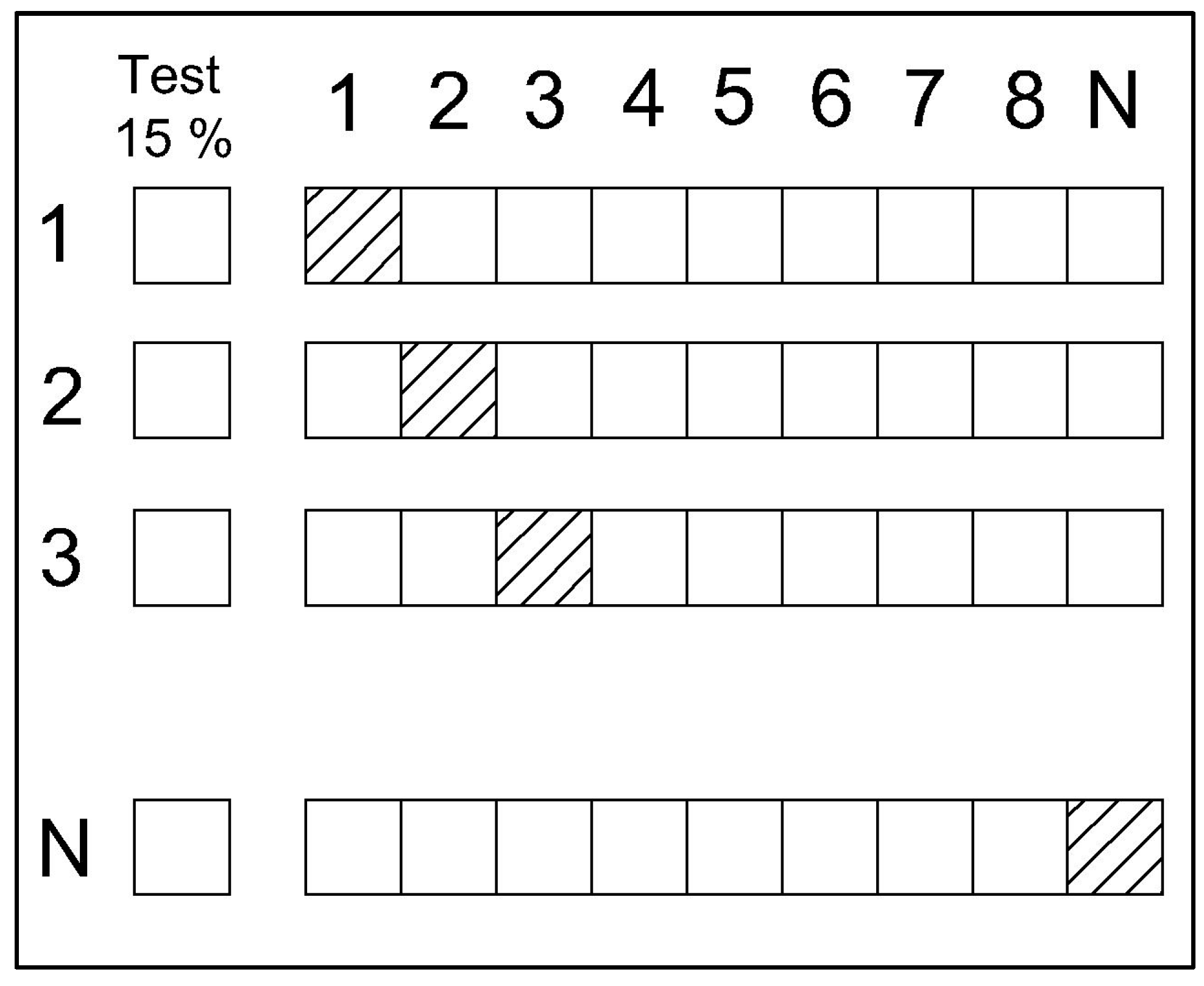
Data analysis based on k-fold validation is shown in Figure 3. As observed, the test data fold amount is kept at 15%. The data arrangement ranges from zero to N number of folds. Each algorithm optimizes and selects a specific number of folds to increase prediction accuracy for the test, validation and training data. Out of each fold, the training and validation data from each subfold are selected to ensure that all the parameters are included in the data analysis part. Furthermore, all the boxes corresponding to each fold are evaluated, and an optimized number of folds are formed with their corresponding MSE and R² values. The shaded portion corresponds to each instance the specific dataset for training and validation was selected for each fold number. Therefore, the hyperparameters optimization related to the fold prediction optimization is carried out to calculate the optimum number of folds for each algorithm, including random forest, SVR, gradient boosting, decision tree, K-neighbour, LightGBM and CatBoost.

4.1. Hyperparameter Optimization

Optimization of hyperparameters using each model is performed where the number of folds is provided, and the optimum number of folds is calculated for each model type used. The range of hyperparameters is chosen based on the number of iterations required for reaching a minimum MSE value; therefore, the following commands are used to calculate the optimum number of folds for hyperparameter optimization. Hyperparameters affect the performance of models in terms of calculated MSE values, with the optimum hyperparameter consisting of the least number of folds for accuracy and time efficiency.

4.1.1. Linear Regression

Number of k-folds = list(range(2, 11)), ‘fit_intercept’: [True, False], ‘copy_X’: [True, False], ‘n_jobs’: [None, −1], ‘positive’: [False, True]

For linear regression, the number of folds between two and eleven is addressed, and parameters including ‘fit_intercept’, ‘copy_X’, ‘n_jobs’ and ‘positive’ are used to optimize the model.

4.1.2. Decision Tree

Number of k-folds = list(range(2, 11)), ‘criterion’: [“squared_error”, “friedman_mse”, “absolute_error”, “poisson”], ‘splitter’: [“best”, “random”], ‘max_depth’: range(3, 26), ‘max_features’: [None, “auto”, “sqrt”, “log2”], ‘min_impurity_decrease’: [0.0, 0.1, 0.2]

For the decision tree algorithm, the number of folds was from two to eleven, and parameters including “squared_error”, “friedman_mse”, ‘splitter’, ‘max_features’ and ‘min_impurity_decrease’ are used to optimize the number of folds with higher prediction accuracy.

4.1.3. Random Forest

Number of k-folds = list(range(2, 11)), ‘criterion’: [“squared_error”, “absolute_error”, “poisson”], ‘max_depth’: [None] + list(range(3, 16))

For the random forest algorithm, the number of folds ranged from two to eleven, with “squared_error”, “absolute_error” and “poisson” used for optimization of number of folds.

4.1.4. Gradient Boosting

Number of k-folds = list(range(2, 11)), ‘learning_rate’: [0.001, 0.01, 0.1, 0.2, 0.3], ‘max_depth’: [3, 4, 5, 6], ‘min_samples_split’: [2, 5, 10], ‘max_features’: [None, ‘sqrt’, ‘log2’], ‘tol’: [1 × 10⁻⁴, 1 × 10⁻³, 1 × 10⁻²], ‘criterion’: [‘friedman_mse’, ‘squared_error’, ‘mse’]

For gradient boosting, the number of folds ranged from two to eleven, with parameters including ‘learning_rate’, ‘max_depth’, ‘max_features’ and ‘mse’ used for optimization.

4.1.5. KNN Regression

Number of k-folds = list(range(2, 11)), ‘n_neighbors’: [3, 5, 7, 9], ‘weights’: [‘uniform’, ‘distance’], ‘algorithm’: [‘auto’, ‘ball_tree’, ‘kd_tree’, ‘brute’], ‘leaf_size’: [20, 30, 40], ‘p’: [1, 2, 3], ‘metric’: [‘euclidean’, ‘manhattan’, ‘chebyshev’, ‘minkowski’]

For KNN regression, the number of k-folds ranged from two to eleven, with parameters including ‘n_neighbors’, weights’, ‘leaf_size’ and ‘metric’ used for further optimization.

4.1.6. SVR

Number of k-folds = list(range(2, 11)), ‘kernel’: [‘linear’, ‘poly’, ‘rbf’, ‘sigmoid’], ‘degree’: [2, 3, 4], ‘gamma’: [‘scale’, ‘auto’, 0.1, 1.0], ‘coef0’: [0.0, 0.1, 0.5], ‘C’: [0.1, 1.0, 10.0]

For SVR, the number of k-folds also ranged from two to eleven, with optimization parameters including ‘kernel’, ‘degree’, ‘gamma’, ‘coef0’ and ‘C’.

5. Data Visualization

In this research, the prediction performance of the models based on fatigue life reduction in years, maximum passes to rut at 6 mm, number of passes to fatigue damage and rut depth at 1.3 million passes is analysed based on the input data used. Different numbers of folds for each model using the k-fold cross-validation technique have been developed.

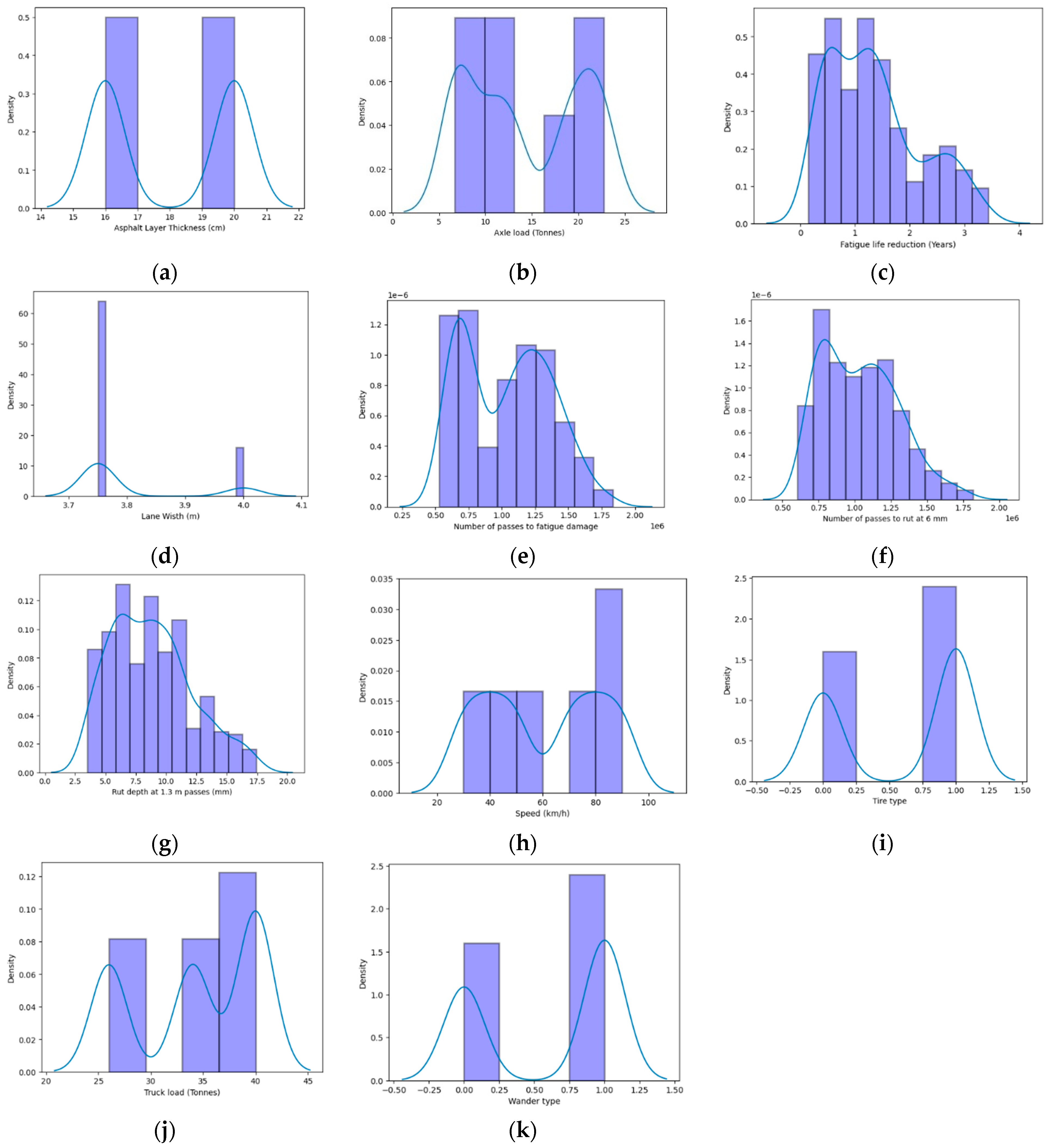
The visualization of data and existing patterns in data are presented. The relationship of input variables and their dependence on each other as well as dependence on output variables are analysed. Frequency of various proportions of input data values including tire types, speed, truck load, axle load, lane width and asphalt layer thickness is evaluated. Furthermore, the frequency and type of input variables used in whole input data series are visualized.

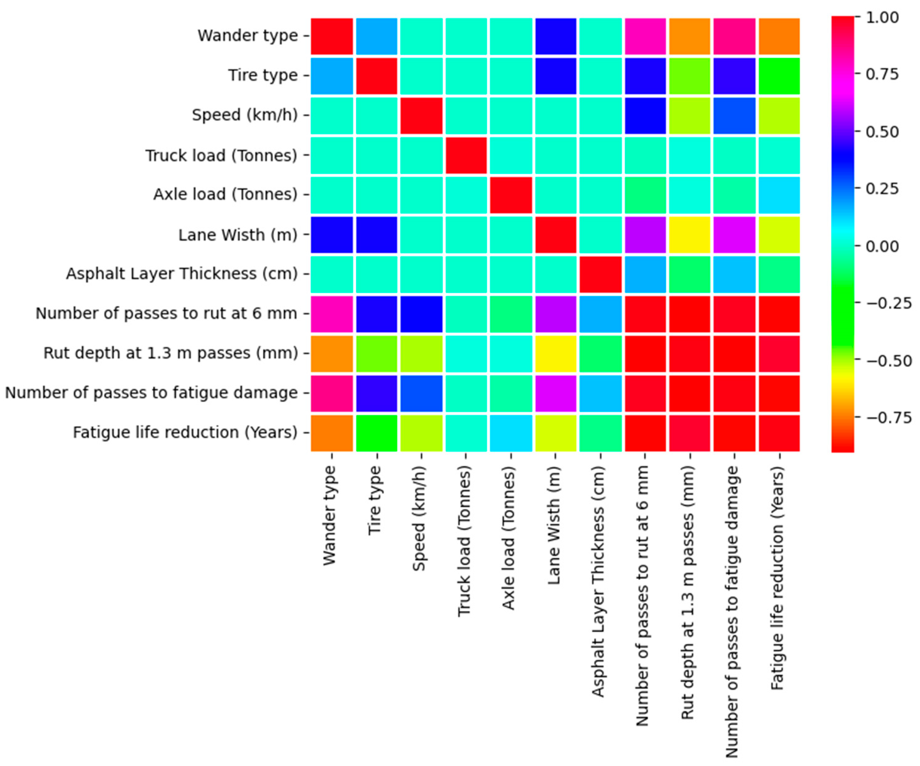
Figure 4 shows the correlation of parameters with a certain degree of dependence based on the colour schemes. Wander type has the highest influence on fatigue life reduction in years. The switch to zero wander mode increases the fatigue life reduction. Furthermore, the increase in speed leads to a decrease in fatigue life reduction, with a correlation value of −0.52. The lane width increment and its relationship with tire type is also visualized. Asphalt layer thickness is not directly related to speed, axle loading and lane width variations. Number of passes to rut depth and number of passes to fatigue damage show the highest relevance with a value of 0.98. The number of passes to fatigue damage and fatigue life reduction behave coherently with a value of −0.89, since fatigue life will decrease with increase in the factor of fatigue life reduction. In terms of rut depth progression, wander type has the highest significance with a factor of −0.72 when switched to uniform wander mode, since the rut depth would decrease. The second most significant parameter affecting the rut depth parameter is the lane width with a factor of −0.59, followed by speed with a value of −0.51.

Correlations of input and output parameters are shown in Figure 5. Furthermore, the relevance of output parameters among one another and the input parameters among one another can be observed. Wander type and fatigue life reduction are inversely related to each other, and the fatigue life reduction would decrease when the uniform wander mode is used. Asphalt layer thickness and number of passes to fatigue and rut depth at 6 mm are in the range of 0.25 with increase in the number of passes at lower asphalt thickness values. Speed has higher significance than the axle load in terms of number of passes to fatigue damage and number of passes to rut depth at 6 mm. Wander type has the highest significance on all the output parameters, since the use of uniform wander or zero wander would significantly affect the pavement distress. Axles load variation does not create a significant difference between rutting and fatigue damage-related output parameters. Lane width increment also affects the rutting and fatigue damage significantly, and the damage increases with reduction in lane width.

Graphical data visualization of input and output parameters is shown in Figure 6. Figure 6a shows the arrangement of asphalt thickness variation in the data used for analysis. The asphalt thickness values ranging from 20 cm to 14 cm are used with decrement of 20 cm, and finite element analysis based on previous research has shown that the ideal use of asphalt layer thickness at 16 cm using 4.2 m of lane width; therefore, most data remain in the vicinity of 16 cm and 20 cm.

According to Figure 6b, based on three different truck types used, the axle load values are used with variations of 6.7 T, 10.6 T, 22.7 T, 7.3 T, 18.7 T, 13 T and 21 T. The frequency of data consisting of axle load greater than 20 T and between 6.7 T and 17 T is higher than that of 18.7 T.

As shown in Figure 6c, fatigue life reduction is provided in terms of the number of reduced years in fatigue life. In most of the scenarios, fatigue life reduction remains at 0.8 years and 1.2 years, individually calculated under each axle. In some instances, where a zero wander mode is used with dual tires at low speeds, the fatigue life reduction reaches 3.3 years.

Since the lane width of 4 m as shown in Figure 6d was found to be ideal for reduced pavement distress for autonomous trucks, only two data variations are provided, consisting of the base scenario of 3.75 m and 4 m.

Based on the effect of parameters including speed, axle type and lateral wander mode type, most of the reduced number of passes to fatigue damage can increase to 1.7 million where zero wander mode is used at low speeds. In the case of a uniform wander mode, the magnitude decreases to 62,000 passes, showing a major shift in the Figure 6e.

As observed from Figure 6f, the highest frequency of data entries exists at 75,000 passes due to the usage of zero wander mode. When uniform wander mode is used as the data move towards the right, a lower number of passes are needed to reach the similar rut depth of 6 mm. In the case of a zero wander mode, around 1.75 million passes are required to reach the rut depth of 6 mm, exhibiting the lowest frequency of data entry.

As observed from Figure 6g, rut depth values are input, ranging from as low as 3.3 mm in cases of uniform wander modes to 17.2 mm in cases of slow speeds at zero wander mode with axle load of 22.7 T. Furthermore, the use of dual tire and zero wander mode significantly increases the rut depth; however, the highest frequency of rut depth inputs remains in the vicinity of 6 mm and 8 mm.

Speed values ranging from 30 km/h to 90 km/h are used for the input data in Figure 6h. However, the higher frequency of speed values at 90 km/h is utilized for assessing the variations in rut depth and fatigue damage values at normal operating speeds.

As observed from Figure 6i, the single wide tire and dual tire types are used for input. The bar line on the left indicates the use of a dual wheel setup, since the single wheel setup is going to be beneficial for the pavement distress; therefore, further data entries for a single wide tire are included for detailed analysis of pavement distress.

As observed from Figure 6j, three different truck types are used for input and analysis based on their GWT. A class-1 type truck has a GWT of 40 T with 5 axles; a class-2 type truck has a GWT of 26 T with 2 axles; and a class-3 type truck has a GWT of 34 T with 4 axles. Since the class-1 type truck has more axles, and it is the truck with the highest percentage in the traffic mix, the frequency of data consisting of class-1 trucks is higher than other two types.

As observed in Figure 6k, data from two lateral wander modes consisting of uniform wander and zero wander modes are included. Since the uniform wander mode performs better than the zero wander mode, it has more data entries for comparisons with other parameters.

6. Results

Prediction of output variables using all the models along with MSE and R² values is presented. Each model uses a specified number of folds based on the extent of output variables. For number of passes to fatigue and rut damage, the MSE increases for all the models; however, when rut depth and fatigue life reduction are evaluated, the MSE stays the minimum. Furthermore, the data scatter for predicted values and actual values is shown along the perfect prediction line. 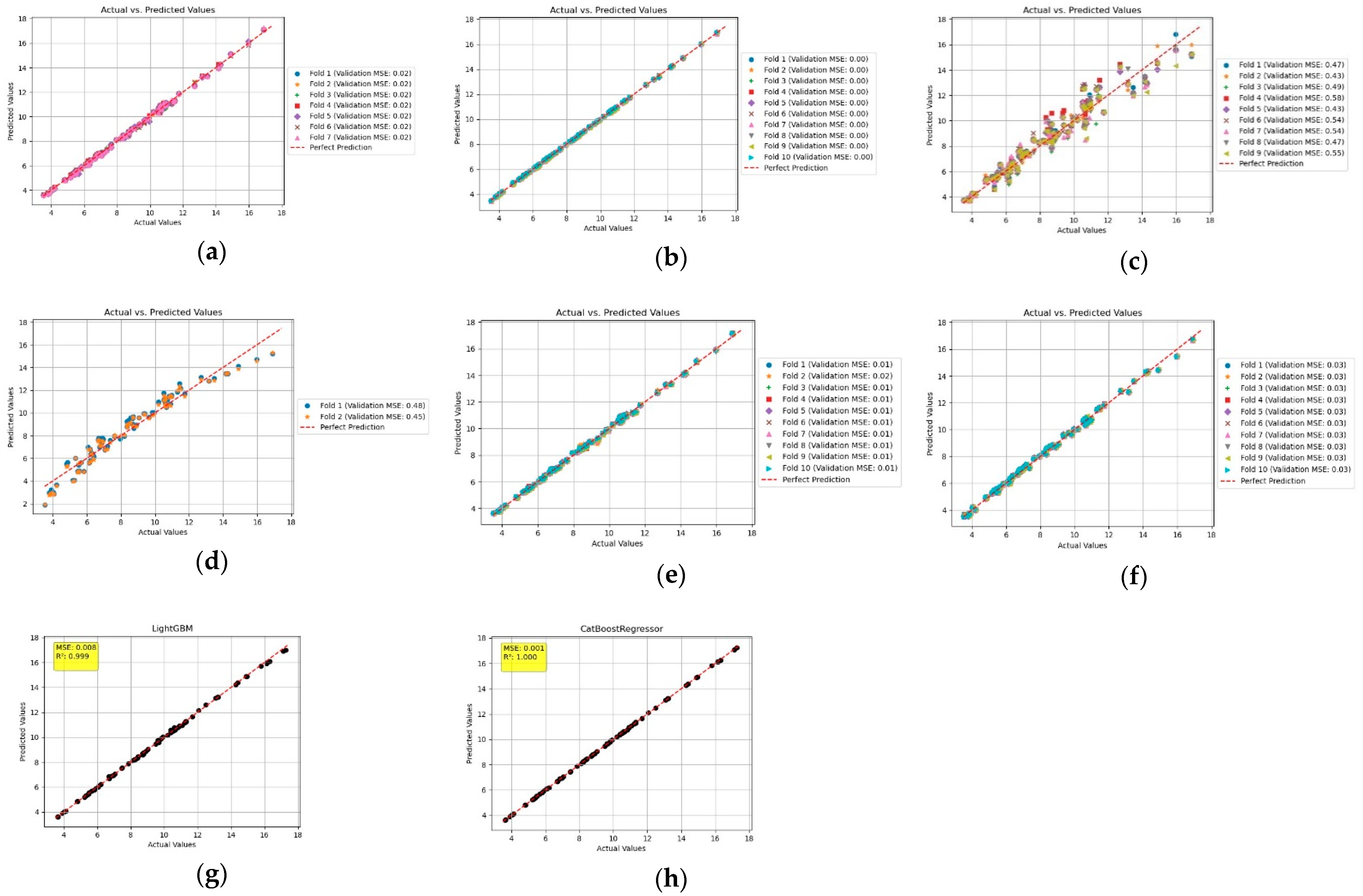Figure 7 shows the performance prediction in terms of fatigue life reduction for different models.

Figure 7a shows comparison of actual calculated and predicted values using the decision tree algorithm. Fatigue life reduction in terms of reduced number of years as a result of zero wander mode are predicted based on the input data. As observed, a total of nine optimized folds are developed using the k-fold technique, and the maximum proficiency of the model was contained against the nine folds. All the folds generate an MSE of 0.00. However, Fold 9 kept the predicted values closer to the actual values.

Figure 7b shows the comparison of values using the gradient boost. As observed, the predicted values lie closer to the centre line, and all folds exhibit the same performance. A total of nine folds have been developed for further optimization of this algorithm.

Figure 7c shows the comparison of predicted reduced fatigue life in number of years and actual fatigue life reduction as used in input using the KNN algorithm. As observed, the predicted values for all the folds are scattered with MSE of 0.04 among all the folds. KNN shows lower performance prediction efficiency as compared to other analysed models.

In Figure 7d, linear regression has been used to evaluate the prediction performance for reduced life in number of years as a result of fatigue damage. A certain pattern can be observed for all the folds analysed using linear regression. Based on the prediction performance evaluation, linear regression yields the minimum MSE of 0.05 for Fold 9 and Fold 3. However, the overall predictive performance of linear regression model is less than that of the K-neighbour algorithm.

In Figure 7e, the random forest algorithm has been used to evaluate the correlation of predicted values with actual values. This algorithm yields the MSE of 0.00 for the majority of folds. However, the scatter in prediction is higher than that of the gradient boosting algorithm.

In Figure 7f, SVR has been used to predict the reduction in fatigue life in years. SVR only requires a total of five folds to perform optimization for a model. Furthermore, SVR yields the MSE of 0.00 for all the folds considered. However, the data scatter is higher than that of the gradient boosting model.

Prediction of reduced fatigue life and comparison with actual values are shown in Figure 7g. As observed, the minimum MSE is obtained at 0.000 and R² of 1.0000. CatBoost regression outperforms other models in terms of prediction accuracy and matching with the actual values for fatigue life reduction in number of years.

Figure 7h above shows the comparison of predicted and actual values using LightGBM. As observed, the model yields accurate results with MSE of 0.001 and R² of 0.999. LightGBM is the second-best machine learning model after CatBoost.

MSE and R² values for prediction of fatigue life reduction in years are shown in

Table 1. MSE and R² values of different models for fatigue life reduction.

Machine Learning Algorithm	MSE	R2
Linear Regression	0.056	0.9023
Decision Tree	0.004	0.9934
Random Forest	0.004	0.9935
Gradient Boosting	0.000	0.9991
KNN	0.037	0.9344
Support Vector Regression	0.004	0.9934
LightGBM	0.001	0.9999
CatBoost	0.000	1.0000
Linear Regression	0.056	0.9023
Decision Tree	0.004	0.9934

. As observed, the highest MSE is shown by linear regression with a value of 0.056 and a corresponding lowest R² value of 0.9023. Furthermore, CatBoost regression exhibits the highest prediction performance among other models with an MSE of 0.000 and R² of 1.000. Gradient boost and LightGBM exhibit the least scatter in predicted data values showing close correspondence to the actual values. However, decision tree, random forest, KNN and SVR also depict good prediction capabilities.

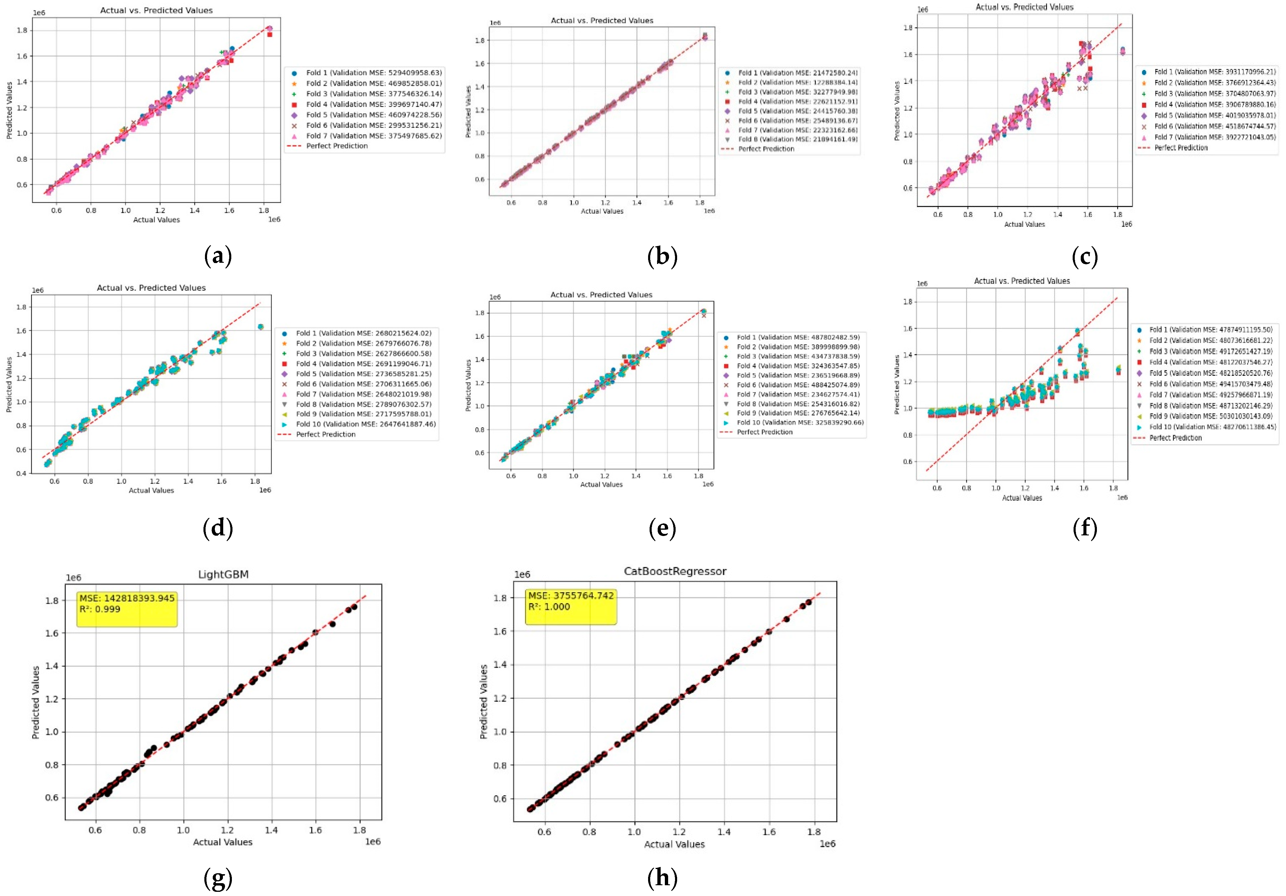
Figure 8 shows the performance prediction in terms of number of passes to fatigue damage for different models. Figure 8a shows the comparison of MSE for predicted and actual values in terms of number of passes to fatigue damage using the decision tree algorithm. Higher magnitude of MSE values correspond to an increased number of passes to fatigue damage in the range of millions. A total of seven folds have been developed. Fold 6 yields the minimum MSE of 299,531,256.21. The decision tree algorithm exhibits increased prediction performance with little scatter at higher number of passes to fatigue.

In Figure 8b, comparison of predicted and actual values is shown using gradient boost. As observed, predicted values stayed on the perfect prediction line exhibiting no scatter. A total of eight folds have been developed. Fold 2 yields the least MSE of 12,288,384.14. Gradient boost outperforms other models with reduced scatter.

In Figure 8c, predicted values are compared against the actual values using the K-neighbour algorithm. Increase in scatter from the actual values can be observed at a higher number of passes. A total of seven folds have been developed, with Fold 7 yielding the minimum MSE of 3,922,721,043.05.

In Figure 8d, predicted values are compared against the actual values using linear regression. Scatter from linear regression is slightly reduced when compared to K-neighbour. Furthermore, MSE has been further reduced to 2,627,866,600.58 at Fold 3. The scatter increases as the number of passes are increased

In Figure 8e, predicted values are compared against the actual values using random forest. A total of 10 folds have been developed, with Fold 7 exhibiting the least MSE of 234,627,574.41. Scatter in predicted values is better than that of KNN and linear regression. Predicted value are at the perfect prediction line at a lower number of passes; however, increase in scatter can be observed at passes more than 1.2 × 10⁶.

In Figure 8f, predicted values are compared against actual values using SVR. As observed, SVR shows the highest scatter and offset in predicted values when compared to actual values among other algorithms. Fold 4 exhibits the least MSE of 48,122,037,546.27.

Performance of LightGBM based on predicted and actual values is shown in Figure 8g. As observed, LightGBM shows overall accurate prediction capacity with slight scatter in prediction along the intermediate and higher number of passes due to non-linear behaviour of asphalt mixture related to fatigue damage. LightGBM yields MSE of 1.428 × 10⁸ and R² of 0.999.

Predicted and actual values for CatBoost regression are shown in Figure 8h. As observed, predicted values stay on the perfect prediction line exhibiting highest prediction performance among other models. Least MSE of 3.755 × 10⁶ is observed with R² of 1.000.

Comparisons of MSE and R² values for number of passes to fatigue damage have been shown in

Table 2. MSE and R² values of different models for number of passes to fatigue damage.

Machine Learning Algorithm	MSE	R2
Linear Regression	2.692 × 109	0.9745
Decision Tree	4.161 × 108	0.9961
Random Forest	3.453 × 108	0.9967
Gradient Boosting	2.285 × 107	0.9998
KNN	3.967 × 109	0.9624
Support Vector Regression	4.874 × 1010	0.5375
LightGBM	1.428 × 108	0.999
CatBoost	3.755 × 106	1.000
Linear Regression	2.692 × 109	0.9745
Decision Tree	4.161 × 108	0.9961

. As observed, CatBoost exhibits the least MSE of 3.755 × 10⁶ and maximum R² of 1.000, followed by LightGBM with MSE of 1.428 × 10⁸ and R² of 0.999. SVR, however, exhibits the highest MSE of 4.874 × 10¹⁰ and R² of 0.5375.

Figure 9 shows the performance prediction in terms of number of passes to reach rut depth of 6 mm for different models. Figure 9a shows the prediction capability of the decision tree algorithm for maximum number of passes to reach rut depth of 6 mm for zero wander mode. Since the number of passes are in the range of a million in some instances, these graphs have been developed and scaled accordingly to exhibit higher MSE values. A total of nine folds for the decision tree algorithm have been developed, and Fold 3 exhibits the least MSE among other folds, with a magnitude of 454,458,547.

Figure 9b shows the prediction of values in terms of number of passes to reach rut depth of 6 mm using gradient boosting. As observed, a total of 10 folds have been developed to further optimize the prediction model. Least MSE is observed at Fold 7, with a value of 22,056,971.7. The graph shows the least amount of data scatter among other algorithms used. Furthermore, the predictive performance of the gradient boosting model surpasses the decision tree algorithm.

In Figure 9c, the predicted values have been plotted against the actual values using the KNN algorithm. Increased data scatter can be observed at a higher number of passes, where rut depth suddenly increases leading to increased prediction deficiency for this model. Least MSE has been observed by Fold 4, with an MSE of 6,335,127,849.05.

Figure 9d shows linear regression being used to predict the values. The scatter pattern is the same as that of the KNN algorithm where scatter increases at a higher number of passes. However, the extent of scatter is less than that of KNN. A total of 10 folds have been developed for model optimization. Least MSE stays at 4,351,218,590.71, which outperforms the prediction capability of the KNN algorithm.

In Figure 9e, predicted values for number of maximum passes to rut depth at 6 mm are shown using random forest. A total of 10 folds have been developed for model optimization. As observed, the random forest algorithm outperforms KNN and linear regression models, exhibiting an MSE of 350,754,482.9.

In Figure 9f, SVR has been used to predict the values for maximum passes to rut depth at 6 mm. As observed, significant increase in data scatter occurs when compared to other algorithms. A total of 10 folds were developed. Fold 3 exhibits the least MSE of 29,456,518,554.68 among other folds. However, the MSE of SVR is significantly higher than other models.

Figure 9g shows the comparison of predicted and actual values for decreased number of passes as a result of fatigue damage. As observed, CatBoost performs well with higher accuracy than other models, yielding the lowest MSE of 5,934,373.659 and R² of 1.000. All the data points stay on the perfect prediction line.

Predicted and actual values from LightGBM are shown in Figure 9h. LightGBM shows overall good performance, with slight scatter in data at mid-range and high-range values. At intermediate and higher numbers of passes, some discrepancy between the predicted and actual values can be observed. However, LightGBM yields MSE of 240,337,676.967 and R² of 0.997.

Comparison of MSE and R² values for maximum number of passes to reach rut depth of 6 mm is shown in

Table 3. MSE and R² values of different models for number of passes to reach rut depth of 6 mm.

Machine Learning Algorithm	MSE	R2
Linear Regression	4.404 × 109	0.9361
Decision Tree	7.349 × 108	0.9893
Random Forest	4.163 × 108	0.9940
Gradient Boosting	3.305 × 107	0.9995
KNN	6.872 × 109	0.9003
Support Vector Regression	2.995 × 1010	0.5656
LightGBM	2.403 × 109	0.997
CatBoost	5.934 × 106	1.000
Linear Regression	4.404 × 109	0.9361
Decision Tree	7.349 × 108	0.9893

. As observed, CatBoost exhibits the least MSE of 5.934 × 10⁶ among other models and a maximum R² of 1.000. Furthermore, the highest MSE exists for SVR, corresponding to a related R² of 0.5656. However, gradient boosting, random forest and LightGBM provide significant prediction capabilities, with R² of 0.9995, 0.9893 and 0.997, respectively, among other algorithms.

Figure 10 shows the prediction performance in terms of rut depth at 1.6 million passes for different models. In Figure 10a, predicted and actual rut depth values based on the number of passes have been shown using the decision tree algorithm. A total of seven folds have been developed, with all folds exhibiting the MSE of 0.02. As observed, predicted values stay closer to the perfect prediction line.

In Figure 10b, gradient boosting has been used to evaluate the predicted and actual values for rut depth. A total of 10 folds have been developed, and all folds exhibit the MSE of 0.00. Gradient boosting outperforms the decision tree algorithm in terms of proximity of data points to the perfect prediction line.

In Figure 10c, the KNN algorithm has been used to compare the predicted value against the actual values. A total of nine folds have been used for model optimization. Fold 2 and Fold 5 exhibit the least MSE of 0.43. However, the data scatter for predicted values is significantly higher than other models. The data scatter increases at higher rut depth values.

In Figure 10d, linear regression has been used to predict the values for rut depth under specified passes and lateral wander type used. Only two folds have been developed for model optimization, and increase in folds did not enhance the model’s prediction capability. Fold 2 exhibits the minimum MSE of 0.45. As observed, the predicted values stay closer to the perfect prediction line around intermediate rut depth values; however, the scatter increases at lower and higher rut depth values. This model outperforms the KNN, but the predictive performance is less than that of gradient boosting and decision tree.

In Figure 10e, the random forest algorithm has been used to predict the values for rut depth based on the input data. A total of 10 folds have been developed for model optimization. Minimum MSE of 0.01 is obtained. Data scatter for random forest corresponds to that of the gradient boosting and decision tree algorithms.

In Figure 10f, SVR has been used to predict the values for rut depth. A total of 10 folds have been used. As observed, data scatter stays closer to the perfect prediction line, leading to an MSE of 0.03 for all the folds. Data scatter increases at higher rut depth values.

Predicted and actual values for rut depth at 1.3 million passes using LightGBM are shown in Figure 10g. As observed, the model exhibits good prediction accuracy, with predicted values staying on the perfect prediction line; however, slight offset from the perfect prediction line can be observed at higher rut depth values. LightGBM exhibits MSE of 0.008 and R² of 0.999.

Figure 10h shows the predicted and actual values using the CatBoost regression. CatBoost outperforms other models in terms of the least MSE of 0.001 and R² of 1.000. As observed, the values stay on the perfect prediction line, with no offset even at higher rut depth values.

MSE and R² for all the models based on rut depth prediction performance have been shown in

Table 4. MSE and R² values of different models for rut depth at 1.6 million passes.

Machine Learning Algorithm	MSE	R2
Linear Regression	0.463450	0.9491
Decision Tree	0.017459	0.9981
Random Forest	0.011836	0.9987
Gradient Boosting	0.000901	0.9999
KNN	0.499082	0.9452
Support Vector Regression	0.030690	0.9966
LightGBM	0.008	0.999
CatBoost	0.001	1.000
Linear Regression	0.463450	0.9491
Decision Tree	0.017459	0.9981

. As observed, CatBoost outperforms other models, with the least MSE of 0.001 and corresponding R² of 1.000. KNN exhibits larger offset of predicted values, with an MSE of 0.499082 and corresponding R² of 0.9452. Prediction performance of LightGBM stays closer to gradient boosting, with MSE of 0.008 and R² of 0.999.

7. Discussion

In this research, different machine learning algorithms have been used to perform performance predictions of asphalt pavement in terms of fatigue damage and rutting. Furthermore, the relationship and dependency between input and output variables have been analysed for 350 data points. K-fold optimization technique has been used to optimize the hyperparameters and the corresponding number of folds for each machine learning algorithm used. The machine learning algorithms used are linear regression, decision tree, random forest, gradient boosting, K-nearest neighbour, SVR, LightGBM and CatBoost. As observed from the results, CatBoost and LightGBM outperform other machine learning models in terms of reduced MSE and R² values. Furthermore, the hyperparameters for LightGBM and CatBoost can be optimized easily with fewer numbers of folds, leading to time efficiency in performance predictions. The least performance is exhibited by linear regression and in some instances by KNN.

In the case of a higher number of passes used both for fatigue damage and rut depth, scatter in the results for SVR increases significantly. KNN and linear regression are also affected by a higher number of passes, where scatter in predicted values increases beyond 1.2 × 10⁶ passes, as shown in Figure 8c and Figure 8d, respectively. Decision tree and random forest show better overall performance than the aforementioned models. CatBoost leads to the use of the minimum number of folds required to reach the minimum MSE of 0.001 in cases of rut depth at 1.6 million passes. Furthermore, LightGBM also exhibits a closer performance to CatBoost in terms of reduced MSE. The inclusion of categorial boosting and arrangement of hyperparameters for both of these models leads to higher prediction efficiency when compared to other models.

Predictive performance of LightGBM is followed by gradient boosting and random forest. CatBoost performs best in all scenarios, whether it is the number of passes to fatigue and rut damage or fatigue and rut life reduction in number of years. Both LightGBM and CatBoost are specific implementations of the gradient boosting machine (GBM) algorithm, which builds trees sequentially by correcting the errors of the previous trees. This iterative correction process helps in reducing bias, leading to better performances as observed in Figure 7g and Figure 7h, respectively. Moreover, LightGBM and CatBoost employ advanced techniques like histogram-based approaches and categorical feature handling (CatBoost), which significantly improve training speed and accuracy. These models are less prone to overfitting compared to simpler models like decision trees because they include regularization techniques like shrinkage (learning rate), early stopping and pruning. Regularization ensures that the models do not memorize the training data but generalize well to unseen data, which is crucial for achieving lower MSE and higher accuracy.

Linear regression assumes that there is a linear relationship between the input features and the target variables. However, in cases like predicting fatigue and rutting damage, the relationship is likely complex and non-linear with high scatter, as shown in Figure 9d. Linear models are unable to capture this complexity, leading to lower accuracy, higher scatter in predictions and increased MSE. This explains why linear regression performs poorly in this context.

K-nearest neighbour works by finding the closest neighbours to a given data point and predicting the output based on their values. While this method can work well for simple datasets, it struggles with high-dimensional or large datasets, particularly when there is noise or irrelevant features. The model has no internal mechanism to handle feature interactions or non-linearity, and its predictions can be highly sensitive to the choice of k (the number of neighbours) and the distance metric. Moreover, KNN can suffer from issues such as overfitting or underfitting, especially if the data have many irrelevant or noisy features, as observed in Figure 10c where the scatter increases with the increase in rut depth magnitude. This leads to reduced prediction accuracy and high variance in its performance.

Decision trees can model complex relationships and non-linear data patterns. However, they have a tendency to overfit the training data if not properly pruned or regularized with less scatter in terms of fatigue life reduction in number of years, as shown in Figure 7a, and rut depth at 1.6 million passes, as shown in Figure 10a. While decision trees provide interpretable results and perform well in capturing feature interactions, their performance often degrades when there is noise in the data.

SVR is designed to model non-linear relationships by mapping the input data to a higher-dimensional space via a kernel function. While SVR can capture complex data patterns, it is highly sensitive to hyperparameters such as the choice of kernel, regularization parameters and the trade-off between bias and variance, leading to further deterioration in prediction performance with very high scatter with higher magnitudes of numbers, as shown in Figure 8f and Figure 9f. If these parameters are not carefully tuned, SVR can underperform, especially in the presence of noisy data or with large datasets. SVR also requires careful preprocessing, like feature scaling, to perform optimally.

Random forest generally performs better than a single decision tree because it averages multiple trees to reduce variance and overfitting. However, it does not take into account the errors of previous trees in the way that gradient boosting, LightGBM and CatBoost do, leading to less refinement in predictions, which can be observed in Figure 9e, in terms of number of passes to reach rut depth of 6 mm. While random forest is robust, less prone to overfitting and more interpretable than other models like SVR, it still cannot reach the accuracy of boosting-based methods in terms of predictive power, particularly in complex, high-dimensional datasets. Random forest benefits from the fact that multiple trees are averaged, reducing variance, but it does not have the advantage of boosting, which can systematically focus on difficult-to-predict cases. Gradient boosting models (like LightGBM and CatBoost) tend to perform better because they correct errors from the previous trees, which allows them to make more refined and accurate predictions. These models can be used for a variety of applications based on the availability of input parameters as used in this research; however, the effect of temperature variations as input variables and their correlation with output variables and the resulting fatigue cracking and rutting damage has not be considered as part of this research, including the use of statistical significance of each model type and error distribution in the prediction evaluation for each model which shall be included in the future research.

8. Conclusions

Since sampling of the training set is further optimized based on the gradient size in the case of LightGBM, it leads to the generation of fewer sampling points when the gradient is calculated. Therefore, LightGBM provides faster training speed with higher accuracy of prediction. LightGBM, CatBoost and gradient boosting are all ensemble models. These models use multiple weak learners (often decision trees) to create a strong learner, improving accuracy and generalization. By combining the results of many trees, these models are able to capture complex patterns in the data that other models do not possess. The findings of this research are as follows:

• CatBoost exhibits the reduced MSE by 188% when compared to linear regression
• The least difference in computed MSE values exists between decision tree and random forest at 38%.
• Gradient boosting, LightGBM and CatBoost exhibit almost similar performance in terms of computed MSE values.
• KNN and linear regression exhibit almost similar performance in terms of computed MSE values.
• Gradient boosting outperforms KNN by 199% in terms of computed MSE.
• The highest R² value is exhibited by LightGBM and CatBoost which is 5% higher than computed R² for linear regression.
• Decision tree, random forest and SVR exhibit almost identical R² values.
• SVR outperforms KNN by 5.2%, marking the highest performance difference between any two algorithms.