Three-Dimensional Inversion of the Time-Lapse Resistivity Method on the MPI Parallel Algorithm

Abstract

The resistivity method is widely used to address long-term monitoring challenges in fields such as environmental protection, ecological restoration, seawater intrusion, and geological hazard assessment. However, external environmental changes can influence monitoring data, resulting in inversion results that fail to accurately reflect subsurface variations. Furthermore, the data volume required for such monitoring is several times larger than that for conventional single-point observations, leading to excessively long inversion times and low computational efficiency. To address these issues, we develop a three-dimensional inversion algorithm for the resistivity method that incorporates time-lapse constraints. Additionally, MPI parallelization is integrated into the program to increase computational efficiency. Through the design of theoretical models and the synthesis of data to test the algorithm, the results show that, compared with those of separate inversion, the shapes and values of time-lapse inversion results at different time points are more consistent, maintaining temporal continuity, and the computational efficiency of MPI parallel inversion is greatly improved. Particularly in high-noise environments, time-lapse inversion effectively suppresses background noise interference, reduces false anomalies, and produces results that closely align with the true model, thus confirming the algorithm’s effectiveness and superiority.

1. Introduction

In recent years, geophysics has been widely used to monitor subsurface changes [1,2,3]. Compared with other geophysical methods, the multielectrode and multichannel system of the resistivity method allows for the effective collection of large-scale monitoring data, offering significant advantages. Therefore, time-lapse resistivity inversion has become a popular topic in geophysical inversion.

The resistivity method has a long history in monitoring [4]. Initially, the international scholar Daily [5] carried out experiments to confirm that the resistivity method could monitor the infiltration process of groundwater, but it involved only repeated measurements at different times, without considering the correlation among the data at those different times. Later, scholars at home and abroad reported that normalizing the observation dataset before inversion, filtering the false anomalies of the initial data, and then applying traditional inversion algorithms could highlight small changes in the physical structure underground [6]. In normalization research, scholars use the inversion results of background data as a priori model to participate in the inversion calculation of subsequent observation data. This approach improves the convergence speed and reduces data fitting errors [7,8,9]. However, these methods do not account for the temporal continuity of physical property changes, making the accurate reflection of subsurface variations challenging. Kim [10] realized time-lapse inversion on the basis of the constraint of time-lapse function. This method simultaneously inverts data from different time points while ensuring that the inversion results evolve continuously over time by constraining datasets at different times. However, time-lapse inversion requires the simultaneous inversion of monitoring data from multiple time points, demanding substantial memory resources and resulting in inefficiencies.

In this study, we developed a three-dimensional inversion algorithm for the resistivity method, that incorporates time-lapse function constraints. We also integrated MPI parallelization into the program to increase computational efficiency, ensuring that the inversion results change continuously over time while significantly improving computational performance. The theoretical model was designed to synthesize data, which confirmed the anti-interference effect of the algorithm.

2. Rationale and Theory

2.1. Three-Dimensional Forward Modeling Algorithm

In this study, the finite difference method is used to implement the three-dimensional forward modeling of the resistivity method. According to the forward modeling theory of the resistivity method derived from Zhu [11], the partial differential equation satisfied by the point source resistivity method is as follows:

$$\nabla \left[\mathit{\sigma }\left(x,y,z\right)\nabla \mathit{\phi }\left(x,y,z\right)\right]=-j\delta (x-x_0)\delta (y-y_0)\delta (z-z_0),$$

(1)

where $\mathit{\sigma }$ is the electrical conductivity of rock ore (S·m⁻¹), $\mathit{\phi }$ is the potential array (V), $j$ is the electric current density (A·m⁻²), and $\delta$ is a Dirac function, that specifies the position of the supply point.

Boundary conditions need to be added at the boundary of infinity and the interface between the surface and air in the meshed region. Boundary conditions are divided into three categories: Dirichlet boundary conditions, Neumann boundary conditions, and mixed boundary conditions.

$$\left\{\begin{array}{l}\phi =0\\ \sigma {\displaystyle \frac{\partial \mathit{\phi }}{\partial n}}=0\\ {\displaystyle \frac{\partial \mathit{\phi }}{\partial n}}+{\displaystyle \frac{\mathit{cos}\theta }{r}}\phi =0\end{array}\right.,$$

(2)

where $n$ is the normal vector outside the boundary, $r$ is the distance from the source point to the boundary, and $\theta$ is the angle between $n$ and $r$.

The Dirichlet boundary condition means that the potential value on the boundary is 0. The Neumann condition boundary condition refers to the normal vector of the current density; that is, the normal derivative of the potential is 0. The mixed boundary condition not only maintains the continuity of the potential at the boundary, but also eliminates the reflection effect on the virtual source at the underground boundary [12,13].The finite difference method is applied to discretize (1), resulting in a large sparse linear system [11], whose matrix form can be expressed as:

$$\mathit{A}\mathit{\phi }=\mathit{b},$$

(3)

where $\mathit{A}$ is the coefficient matrix, which is used to calculate the sparse matrix of each element through the finite difference method and then assemble it into a large coefficient matrix of all the elements; $\mathit{b}$ is the vector that contains information with respect to the field source.

The potential is obtained by solving (3) using the BICGSTAB method. After the potential is obtained, the apparent resistivity is obtained according to (4).

$$\left\{\begin{array}{l}\mathit{U}=\mathit{\alpha }\mathit{\phi }\\ {\rho }_a=K{\displaystyle \frac{\mathrm{\Delta }\mathit{U}}{I}}\end{array}\right.,$$

(4)

where $\mathit{\alpha }$ is the vector that is designed to select the potential at the receiver among all grid node potentials, $\mathrm{\Delta }\mathit{U}$ is the potential difference between the receiving electrodes (V), $I$ is the electric current (A), and $K$ is the geometric factor.

In this study, the accuracy and precision of the finite difference method are verified. A vertical contact band model is designed, as shown in Figure 1, in which the dielectric resistivity on the left is 100 Ω·m, and the dielectric resistivity on the right is 20 Ω·m. Data acquisition is carried out using a three-pole device, where A represents the transmitting electrode, M and N represent the receiving electrode, and observations are made from left to right.

Figure 2 shows the apparent resistivity curve of the vertical contact zone model. The numerical solution obtained by numerical simulation using the finite difference method is close to the analytical solution, and the error of both methods is less than 5% at all measurement points, which verifies the accuracy and precision of the forward numerical simulation results in this paper.

2.2. Time-Lapse Function

The time-lapse function ensures the continuity of the inversion results across different times. In the process of time-lapse inversion, the data at different times are synchronously inverted. Assuming that ${\mathit{m}}_{\mathit{\sigma },\mathit{i}}$ is the conductivity model at a certain time, the time-lapse conductivity model ${\mathit{M}}_{\mathit{\sigma }}$ can be defined as:

$${\mathit{M}}_{\mathit{\sigma }}={\left[{\mathit{m}}_{\mathit{\sigma },1} {\mathit{m}}_{\mathit{\sigma },2} \dots {\mathit{m}}_{\mathit{\sigma },\mathit{n}\mathit{t}}\right]}^T,$$

(5)

where $\mathit{n}\mathit{t}$ is the number of observations. At present, there are two calculation methods for time-lapse function: L1 norm and L2 norm [14,15]. The time-lapse function calculated by the L2 norm can better ensure the continuity of inversion results over time, whereas the time-lapse function calculated by the L1 norm can avoid the over-continuity of inversion results at different times with time and better reflect the local changes at different times [16]. In this study, we focus on the anti-interference effect of the time-lapse function on high noise, so the L2 norm method is used for calculation, and the calculation formula is as follows:

$${\Phi }_t({\mathit{M}}_{\mathit{\sigma }})={\mathit{M}}_{\mathit{\sigma }}^{\mathit{T}}{\mathit{C}}^{\mathit{T}}\mathit{C}{\mathit{M}}_{\mathit{\sigma }}={\sum }_{k=1}^{nt}{‖{\mathit{m}}_{\mathit{\sigma },\mathit{k}}-{\mathit{m}}_{\mathit{\sigma },\mathit{k}+1}‖}^2,$$

(6)

$$\mathit{C}=\left[\begin{array}{c}{I}_{1 }\hspace{0.33em}-I_2\hspace{0.33em}0\hspace{0.33em}\hspace{0.33em}\hspace{0.33em}0\hspace{0.33em}\hspace{0.33em}\hspace{0.33em}\hspace{0.33em}0\\ 0\hspace{0.33em}\hspace{0.33em}\hspace{0.33em}\hspace{0.33em}{I}_2\hspace{0.33em}\hspace{0.33em}\hspace{0.33em}-I_3\hspace{0.33em}\hspace{0.33em}0\hspace{0.33em}\hspace{0.33em}\hspace{0.33em}\hspace{0.33em}0\\ 0\hspace{0.33em}\hspace{0.33em}\hspace{0.33em}\hspace{0.33em}0\hspace{0.33em}\hspace{0.33em}\ddots \hspace{0.33em}\hspace{0.33em}\ddots 0\hspace{0.33em} \hspace{0.33em}\hspace{0.33em}0\\ 0\hspace{0.33em}\hspace{0.33em}\hspace{0.33em}\hspace{0.33em}0\hspace{0.33em}\hspace{0.33em}\hspace{0.33em}\hspace{0.33em}0\hspace{0.33em}\hspace{0.33em}{I}_{\mathrm{nt}-1}\hspace{0.33em}{I}_{\mathrm{nt}}\end{array}\right],$$

(7)

where ${\Phi }_t\left({\mathit{M}}_{\mathit{\sigma }}\right)$ is a time-lapse function, which is calculated by the difference in the underground conductivity model at the adjacent time. By introducing the time-lapse function into the objective function, the difference in the inversion results at the adjacent time can be reduced by minimizing the objective function, to ensure that the underground physical property model changes continuously with time.

2.3. Three-Dimensional Time-Lapse Inversion Objective Function

In this study, we use the regularized constrained inversion method, which adds model terms to the objective function to constrain, avoiding excessive data fitting and reducing the multiplicity of geophysical inversion solutions. The objective function of regularization constraint inversion is as follows:

$$\Phi \left({\mathit{M}}_{\mathit{\sigma }}\right)={\Phi }_d\left({\mathit{M}}_{\mathit{\sigma }}\right)+{\lambda }_m^{\sigma }{\Phi }_m\left({\mathit{M}}_{\mathit{\sigma }}\right),$$

(8)

The objective function consists of two parts: the data function ${\Phi }_d\left({\mathit{M}}_{\mathit{\sigma }}\right)$ and the model function ${\Phi }_m\left({\mathit{M}}_{\mathit{\sigma }}\right)$. ${\Phi }_d\left({\mathit{M}}_{\mathit{\sigma }}\right)$ is used to calculate the difference between the observation data and the response data of the inversion result, ${\Phi }_m\left({\mathit{M}}_{\mathit{\sigma }}\right)$ is used to calculate the smoothness of the model, and ${\lambda }_m^{\sigma }$ is the weight factor of the model function, which is used to adjust the proportions of the data function and the model function in the objective function.

By introducing the time-lapse function calculated by (6) into (8), the time-lapse inversion objective function can be obtained:

$$\Phi \left({\mathit{M}}_{\mathit{\sigma }}\right)={\Phi }_d\left({\mathit{M}}_{\mathit{\sigma }}\right)+{\lambda }_m^{\sigma }{\Phi }_m\left({\mathit{M}}_{\mathit{\sigma }}\right)+{\lambda }_t^{\sigma }{\Phi }_t\left({\mathit{M}}_{\mathit{\sigma }}\right),$$

(9)

where ${\lambda }_t^{\sigma }$ is the weight factor of the time-lapse function.

In this study, we use the method of L-curves to choose the ${\lambda }_m^{\sigma }$ and ${\lambda }_t^{\sigma }$ [17], which can not only ensure the minimum of ${\Phi }_d\left({\mathit{M}}_{\mathit{\sigma }}\right)$, but also ensure the minimum of ${\Phi }_m\left({\mathit{M}}_{\mathit{\sigma }}\right)$ and ${\Phi }_t\left({\mathit{M}}_{\mathit{\sigma }}\right)$.

Expanding (9) yields the specific form of the time-lapse inversion objective function:

$$\Phi ({\mathit{M}}_{\mathit{\sigma }})={\left[{\mathit{D}}_{\mathit{\rho },\mathit{o}\mathit{b}\mathit{s}}-\mathit{F}\left({\mathit{M}}_{\mathit{\sigma }}\right)\right]}^T{\mathit{V}}_{\mathit{\sigma }}^{-1}\left[{\mathit{D}}_{\mathit{\rho },\mathit{o}\mathit{b}\mathit{s}}-\mathit{F}\left({\mathit{M}}_{\mathit{\sigma }}\right)\right]+{{\lambda }_m^{\sigma }({\mathit{M}}_{\mathit{\sigma }}-{\mathit{M}}_{\mathit{\sigma },0}{)}^T\mathit{C}}_{\mathit{M},\mathit{\sigma }}^{-1}({\mathit{M}}_{\mathit{\sigma }}-{\mathit{M}}_{\mathit{\sigma },0})+{\lambda }_t^{\sigma }{\mathit{M}}_{\mathit{\sigma }}^{\mathit{T}}{\mathit{C}}^{\mathit{T}}\mathit{C}{\mathit{M}}_{\mathit{\sigma }},$$

(10)

where ${\mathit{D}}_{\mathit{\rho },\mathit{o}\mathit{b}\mathit{s}}$ represents the apparent resistivity data observed at all times, $\mathit{F}\left({\mathit{M}}_{\mathit{\sigma }}\right)$ represents the forward response function, ${\mathit{M}}_{\mathit{\sigma },0}$ represents the initial model of inversion, and ${\mathit{V}}_{\mathit{\sigma }}$ represents the covariance matrix of the data. The gradient of the objective function can be obtained by calculating the partial derivative of the objective function with respect to ${\mathit{M}}_{\mathit{\sigma }}$:

$$g\left({\mathit{M}}_{\mathit{\sigma }}\right)=-2{\mathit{J}}_{\mathit{\sigma }}^{\mathit{T}}{\mathit{V}}_{\mathit{\sigma }}^{-1}\left[{\mathit{D}}_{\mathit{\rho },\mathit{o}\mathit{b}\mathit{s}}-\mathit{F}\left({\mathit{M}}_{\mathit{\sigma }}\right)\right]+2{\lambda }_m^{\sigma }{\mathit{C}}_{\mathit{M},\mathit{\sigma }}^{-1}\left({\mathit{M}}_{\mathit{\sigma }}-{\mathit{M}}_{\mathit{\sigma },0}\right)+2{\lambda }_t^{\sigma }{\mathit{M}}_{\mathit{\sigma }}^{\mathit{T}}{\mathit{C}}^{\mathit{T}}\mathit{C}{\mathit{M}}_{\mathit{\sigma }},$$

(11)

where $J_{\sigma }$ represents the sensitivity matrix of the inversion.

Owing to the complexity of the underground model and observation data, it is necessary to smooth the gradient of the objective function to improve the computational efficiency and stability of the inversion. Egbert and Kelbert proposed a simple and efficient method to smooth the gradient of model parameters [18]. The specific transformation formula is derived as follows:

$$\left\{\begin{array}{c}{\mathit{C}}_{\mathit{M},\mathit{\sigma }}^{-1}={{(\mathit{C}}_{\mathit{M},\mathit{\sigma }}^{-1/2})}^{\mathit{T}}{\mathit{C}}_{\mathit{M},\mathit{\sigma }}^{-1/2}\\ {\tilde{\mathit{M}}}_{\mathit{\sigma }}={\mathit{C}}_{\mathit{M},\mathit{\sigma }}^{-1/2}({\mathit{M}}_{\mathit{\sigma }}-{\mathit{M}}_{\mathit{\sigma },0})\end{array}\right.,$$

(12)

Formula (11) is transformed by the method above to obtain:

$$g\left({\tilde{\mathit{M}}}_{\mathit{\sigma }}\right)=-2{\mathit{C}}_{\mathit{m},\mathit{\sigma }}^{1/2}{\mathit{J}}_{\mathit{\sigma }}^{\mathit{T}}{\mathit{V}}_{\mathit{\sigma }}^{-1}\left[{\mathit{D}}_{\mathit{\rho },\mathit{o}\mathit{b}\mathit{s}}-\mathit{F}\left({\mathit{M}}_{\mathit{\sigma }}\right)\right]+{2\lambda }_m^{\sigma }{\tilde{\mathit{M}}}_{\mathit{\sigma }}+2{\lambda }_t^{\sigma }{\mathit{C}}_{\mathit{m},\mathit{\sigma }}^{1/2}{\mathit{C}}^{\mathit{T}}\mathit{C}\left({\mathit{C}}_{\mathit{m},\mathit{\sigma }}^{1/2}{\tilde{\mathit{M}}}_{\mathit{\sigma }}+{\mathit{M}}_{\mathit{\sigma },0}\right),$$

(13)

After ${\tilde{\mathit{M}}}_{\mathit{\sigma }}$ is obtained through inversion, the model ${\mathit{M}}_{\mathit{\sigma }}$ is solved by the following inverse transformation method:

$${\mathit{M}}_{\mathit{\sigma }}={\mathit{C}}_{\mathit{M},\mathit{\sigma }}^{1/2}{\tilde{\mathit{M}}}_{\mathit{\sigma }}+{\mathit{M}}_{\mathit{\sigma },0},$$

(14)

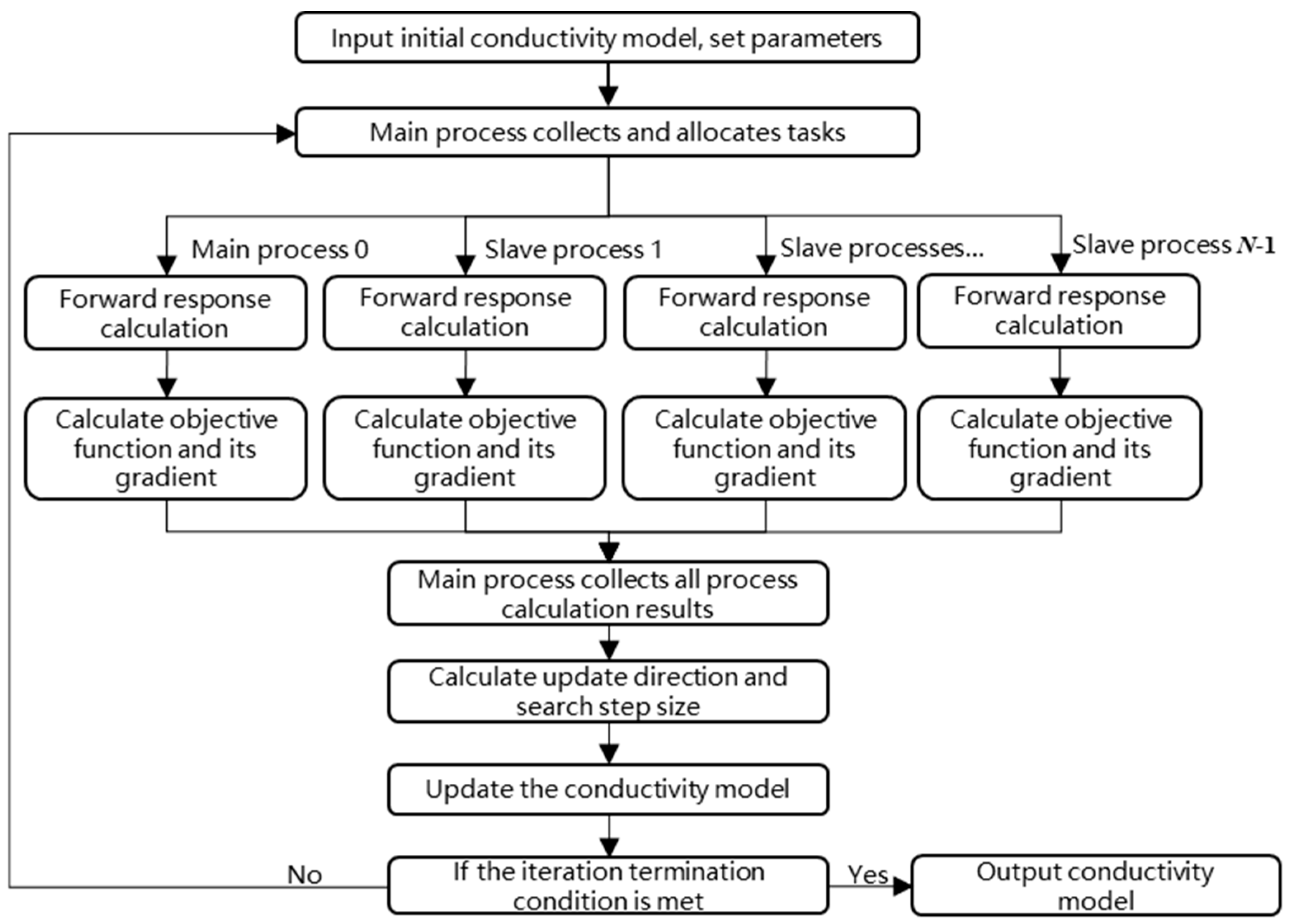
2.4. MPI Parallel Inversion Algorithm

To better reflect the subsurface information, three-dimensional inversion via the resistivity method uses multiple point power sources to improve the inversion performance. The corresponding amount of observation data is large, and the original serial inversion program is inefficient. When calculating the forward response, apparent resistivity, and potential at various measuring points for different power supply points, the Jacobian matrix corresponding to each source point during gradient calculation and the solution of the quasi-forward equations are independent of one another. Therefore, the problem can be divided into several independent subproblems, and parallel computing can enhance the inversion speed and efficiency. MPI is not a language, but rather a “function library” that can be applied to a variety of programming languages and contains hundreds of functions calling interfaces.

Table 1. The parallel environment-related library functions used in the programming process.

Function Name	Functions
MPI_INIT	Initializes all MPI programs.
MPI_FINALIZE	Finalizes all MPI programs.
MPI_COMM_RANK	Returns the identification number for calling a process in a given communication domain, distinguishing different processes from other processes.
MPI_COMM_SIZE	Returns the number of included processes in a given communication domain.

lists the parallel environment-related library functions used in the programming process.

In parallel inversion, the main process communicates with sub-processes. The sub-processes communicate with each other, and transmit messages and data, including three parts: message assembly, message passing, and message receiving.

Table 2. Library functions related to communication.

Function Name	Functions
MPI_SEND	Sends the data in the buffer to the destination child process.
MPI_RECV	Receives information from the specified process.
MPI_BCAST	Sends a message from the main process to all child processes in the group that includes itself.
MPI_ ALLGATHER	Make each child process collect data from all other processes.

shows the library functions related to communication.

The MPI parallel algorithm significantly improves computational efficiency through the synchronous allocation of tasks across multiple processes. It includes both peer-to-peer and master–slave modes. In the peer-to-peer mode, all processes contribute to completing a portion of the assigned tasks. In the master–slave mode, processes are divided into master and slave processes. The master process is responsible for task allocation, message transmission, and data collection, whereas the slave processes execute the assigned tasks. In this study, the master–slave mode is selected. Suppose that there are 4 field sources, and that 10 data points are observed for each field source. N processes are used for calculations using MPI, with each process assigned 40/N field source calculation tasks. Finally, the MPI parallel algorithm is integrated into the inversion algorithm, forming a 3D time-lapse inversion MPI parallel algorithm suitable for combined data from multiple devices via the resistivity method. The MPI parallel inversion flow chart for the resistivity method is shown in Figure 3.

The flow chart can be briefly summarized in the following steps:

(1) The initial conductivity is inputted, and the necessary parameters for inversion are set.

(2) The main process collects and assigns tasks to slave processes.

(3) The calculation of the forward response between the master and slave processes is synchronized, and the computation of the objective function and gradient continues.

(4) The main process collects the results from all the processes.

(5) The update direction is calculated, and the step size is determined.

(6) The conductivity model is updated.

(7) The iteration termination criteria are checked. If the criteria are met, the iteration terminates; if not, the iteration continues.

(8) The termination criteria of inversion are when the data misfit is below a predefined threshold or the number of iterations reaches a set limit. The formula for calculating the misfit (root mean square, RMS) is as follows:

$$RMS=\sqrt{{\displaystyle \frac{{\left[{\mathit{D}}_{\mathit{\rho },\mathit{o}\mathit{b}\mathit{s}}-\mathit{F}\left({\mathit{M}}_{\mathit{\sigma }}\right)\right]}^T{\mathit{V}}_{\mathit{\sigma }}^{-1}\left[{\mathit{D}}_{\mathit{\rho },\mathit{o}\mathit{b}\mathit{s}}-\mathit{F}\left({\mathit{M}}_{\mathit{\sigma }}\right)\right]}{N}}},$$

(15)

where $N$ is the number of data points.

In this study, the termination condition is set such that RMS is less than 1 or the number of iterations is greater than 100.

3. Synthetic Example Tests

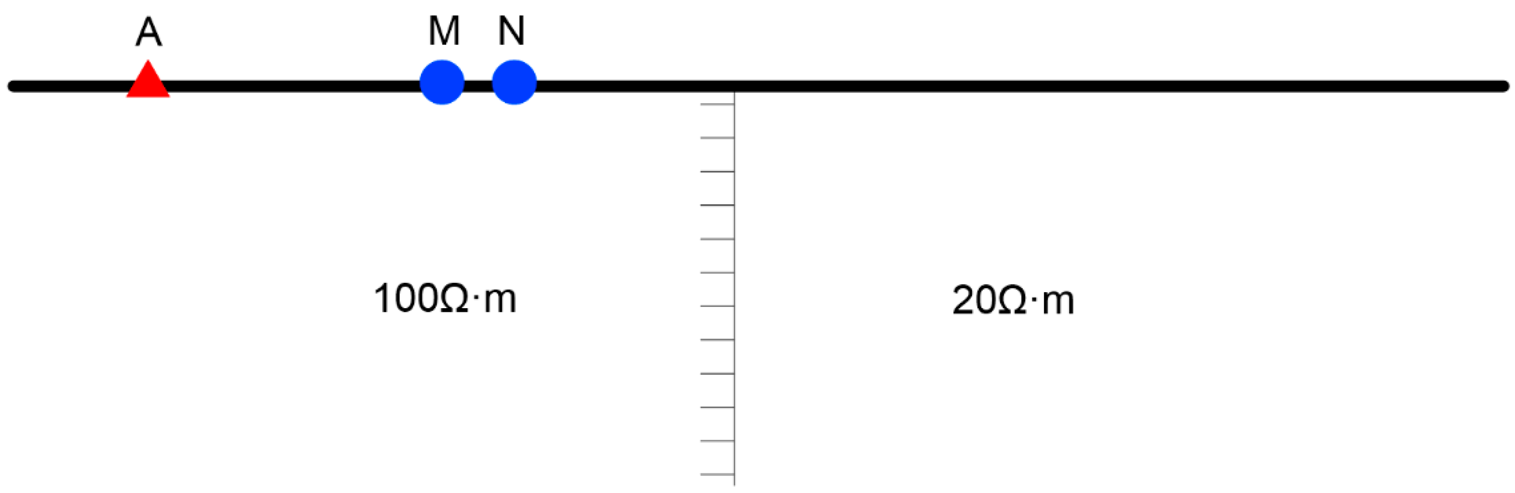
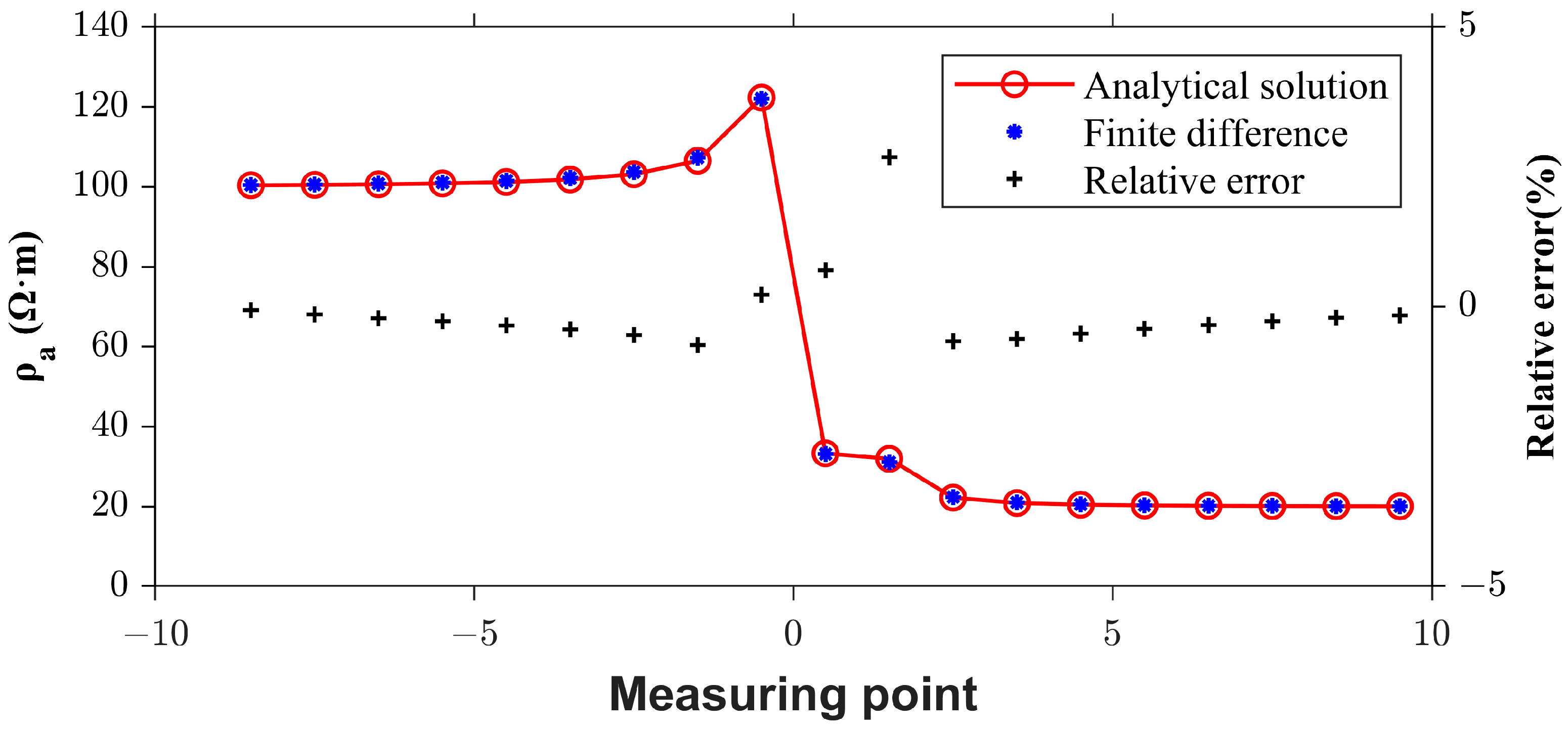
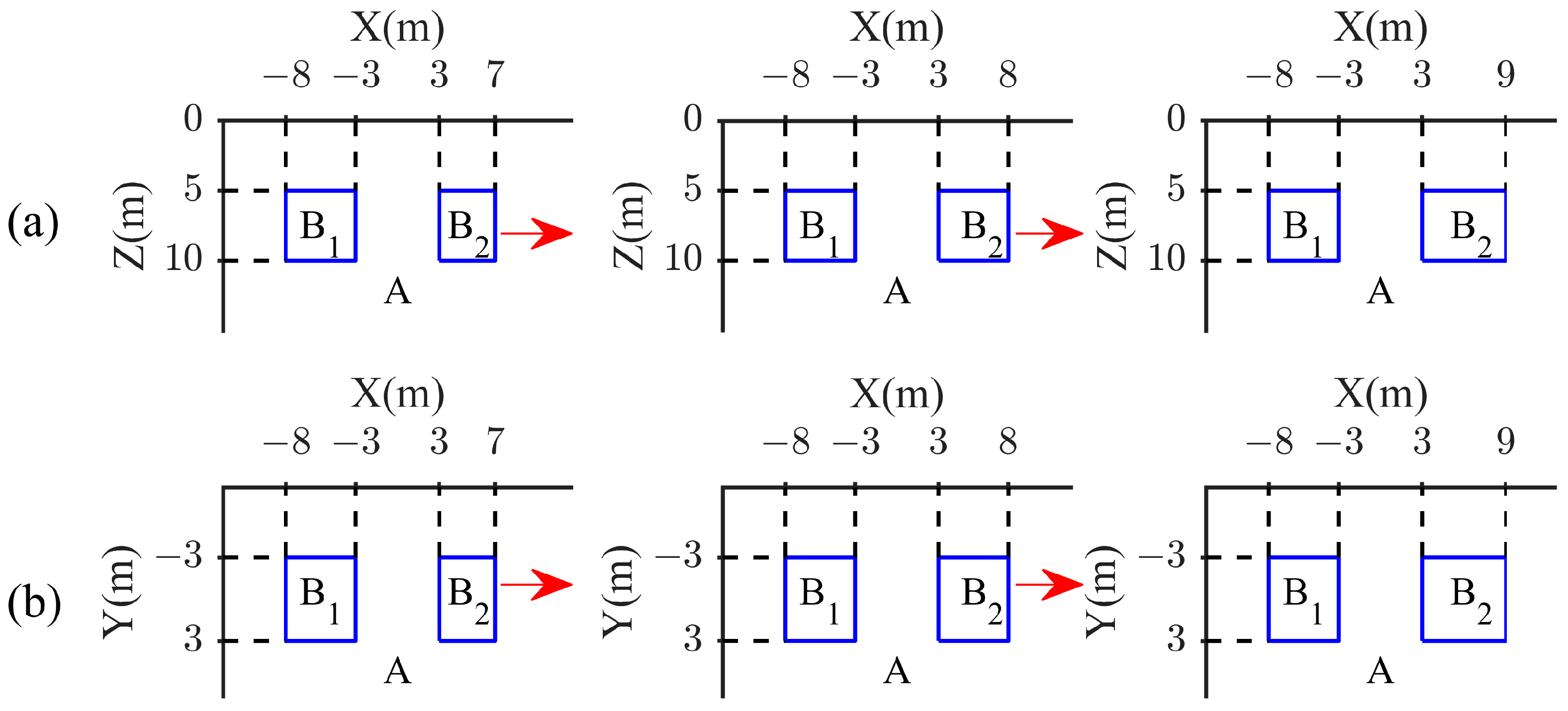
3.1. Theoretical Model and Forward Modeling Response

The time-lapse resistivity method is commonly used to monitor the migration process of underground fluid, in which the fluid often migrates from one geological unit to another with groundwater. In this study, a time-lapse model is established to simulate the fluid migration process.

Figure 4 shows the sections of the time-lapse model. The anomalous bodies in the time-lapse model are two low-resistance prisms. The left prism remains unchanged, whereas the prism on the right diffuses along the positive direction of the X-axis, simulating the continuous migration of underground fluids over time. The time-lapse model includes three different time points, labeled T₁, T₂, and T₃. A schematic diagram of the model in the X–Z and X–Y directions at these three times is shown from left to right. The resistivity of background A is 100 Ω·m, whereas the resistivities of abnormal bodies B₁ and B₂ are 10 Ω·m. The size of B₁ is fixed, with dimensions of 5 m in the X-direction, 6 m in the Y-direction, and 5 m in the Z-direction. The distance between B₁ and B₂ is 6 m. B₂ remains fixed at 6 m in the Y-direction and 5 m in the Z-direction, but its size in the X-direction increases over time, reaching 4 m, 5 m, and 6 m at T₁, T₂, and T₃, respectively.

The same observation system was used for forward modeling of the time-lapse model at T₁, T₂, and T₃. Figure 5 shows a schematic diagram of the observation system. The three-pole device is used for measurement on the ground surface. The electrodes are arranged as a rectangular square array, the red triangle represents the position of the transmitting electrode, the blue dot represents the position of the receiving electrode, and the black solid line box represents the projection of the anomalous bodies B₁ and B₂ on the ground surface. When each transmitting electrode is powered, all adjacent receiving electrodes in the X-direction are activated to ensure that enough information in the three-dimensional space is obtained. Gaussian-random errors of 5%, 5%, and 20% were added to the observation data at T1, T2, and T3, respectively, which simulated significant noise disturbance in the data. At last, there were a total of 194 sources, with 23,760 data points obtained at a single time, and 71,280 data points obtained at three times.

The forward modeling and inversion use the same grid generation method, which is obtained through many forward and inversion tests. First, we must ensure that all the transmitting and receiving electrodes are on the grid nodes; second, infinity is set to more than 3 times the size of the observation area; finally, we must ensure that there are at least 1–2 lines with 3–5 points on each line above the anomalous body.

3.2. MPI Parallel Calculation Efficiency

We evaluate the computational efficiency of the three-dimensional MPI parallel inversion via the time-lapse resistivity method. Taking the above synthetic data as an example, with consistent grid division, inversion of the initial model, and observation data errors, the program was executed using 5, 10, 20, 30, and 40 processes, respectively, and the times of the serial program were compared. Table 1 shows the running times of the serial program and the MPI parallel program.

As shown in

Table 3. Comparison of the running time of the serial program and the MPI parallel program.

Type of Program	Number of Processes	Running Time /Minutes	Acceleration Ratio
Serial program	1	487.26	1
MPI parallel program	5	124.3	3.92
	10	64.62	7.54
	20	36.77	12.98
	30	32.46	15.04
	40	31.32	15.56

, the relative acceleration ratio between the MPI parallel program and serial programs is not an integer multiple relationship. When the number of processes is 5, the acceleration ratio increases greatly. As the number of processes increases, the growth rate of the acceleration ratio decreases. When the number of processes is 40, the acceleration ratio is almost unchanged compared with when the number of processes 30. This has two causes. First, during the execution of parallel programs, data transfer between processes takes up time, decreasing efficiency. Second, only processes with high computational complexity such as forward response, objective functions, and gradients need to use MPI parallel computing; the other processes do not need to use MPI parallel programs. Overall, a reasonable number of processes can not only ensure the improvement of computing efficiency but also avoid the waste of computer processes. In practice, we should set the number of processes reasonably according to the specific number of sources.

3.3. Analysis of the Inversion Results

We performed both separate inversion and time-lapse inversion on the synthesized data. The final RMS values of single inversion and time-lapse inversion are 1.77 and 1.76, respectively. Compared with that of single inversion, the RMS of time-lapse inversion is slightly smaller because the RMS reflects only the degree of data fitting. In this study, we added high noise to the data, so the RMS value cannot accurately invert the true fitting degree of the true resistivity model.

Figure 6 and Figure 7 show the sections at Z = 8 m and Y = 0 m for the separate inversion and time-lapse inversion results, respectively. The black solid line in the figures represents the true location of the anomalous bodies.

The analysis of the results shown in Figure 6 and Figure 7 clearly reveals that the time-lapse inversion results are more similar in shape and resistivity values for anomalous bodies B₁ and B₂ at all three times than the separate inversion results are.

The results of the separate inversion and time-lapse inversion at the three times points were compared. At T₁, the time-lapse inversion better approximates the shape and resistivity of anomalous body B₂ than the separate inversion does. At T₂, there is no significant change in the shape or resistivity of anomalous bodies B₁ and B₂ between the time-lapse and separate inversions. At T₃, the separate inversion results are heavily influenced by noise, distorting the shapes of B₁ and B₂ and introducing false anomalies around the anomalous bodies. In contrast, the time-lapse inversion significantly reduces these distortions and eliminates most of the false anomalies.

To further assess the constraint effect of the time-lapse function, we computed the difference between adjacent time points for both the separate inversion results and the time-lapse inversion results, as shown in Figure 8 and Figure 9. The black solid line represents the model from the previous time step, and the area between the black solid line and the dotted line highlights the model changes relative to the previous time.

As shown in Figure 8 and Figure 9, the resistivity difference between adjacent times decreases after time-lapse inversion. At the Z = 8 m section, the resistivity of the T₂–T₁ model significantly decreases in the real change area after separate inversion, and the reduction range is larger than that in the real change area. The resistivity of the T₃–T₂ model changes in a disordered manner, which is inconsistent with the real change area and is caused mainly by the influence of high noise at T₃. After time-lapse inversion, the variation ranges of the resistivities of the T₂–T₁ and T₃–T₂ models are on the right side of the real variation area, and the variation value is smaller, whereas the variation range of the resistivities of the T₃–T₂ models is more regular. At the Y = 0 m section, the resistivity of T₂–T₁ and T₃–T₂ decreases around B₂ after separate inversion, and the variation range is larger than the real variation region. After time-lapse inversion, the variation range of the resistivity is smaller, and it is concentrated in the upper right of the real variation region.

To quantitatively evaluate the effect of time-lapse inversion, the model fitting difference $\delta$ is introduced to calculate the difference between the real model and the inversion result. The calculation of model fitting difference $\delta$ follows the calculation method of Moorkamp [19].

$$\delta ={\displaystyle \frac{1}{M_p}}\sqrt{{{\sum }_{i=1}^{M_p}\left({\displaystyle \frac{m_i^{inv}-m_i^{true}}{m_i^{true}}}\right)}^2},$$

(16)

where $m_i^{true}$ represents the true model, $m_i^{inv}$ represents the result of the separate method or joint inversion, and $M_p$ represents the total number of grid cells underground.

Table 4. The $\delta$ value of separate inversion and time-lapse inversion.

Parameter	Model	Separate Inversion	Time-Lapse Inversion
$\mathit{\delta }$	T1	6.15	5.95
	T2	5.41	5.48
	T3	5.35	4.12

shows the δ value statistics of the results of single inversion and time-lapse inversion. We can use (16) to calculate $\delta$ at three times.

Compared with those of the single inversion, the $\delta$ value at T₁ decreases, the $\delta$ value at T₂ increases, and the $\delta$ value at T₃ decreases after time-lapse inversion. This is because the resistivity values at the three times in the time-lapse model have not recovered to the true value; with increasing B₂ scale, the resistivity value decreases, and the time-lapse inversion results in closer values at those three times. At T₁, the resistivity of B₂ decreases and is closer to the true value, resulting in a decrease in the $\delta$ value at T₁. At T₂, the $\delta$ value increases because of the influence of high-noise data at T₃. The influence of noise at T₃ is suppressed by T₂, and the $\delta$ value also decreases.

In summary, the inversion results of time-lapse inversion at adjacent times are more similar in value form and can still reflect the change in underground resistivity under high noise interference.

4. Conclusions

In this study, a three-dimensional inversion of the time-lapse resistivity method based on time-lapse function constraint theory was implemented, and an MPI parallel design was incorporated into the program.

Using synthetic data from the theoretical model, both separate inversion and time-lapse inversion were conducted to test the program. The MPI parallel design significantly reduces the program runtime, which is critical for geophysical monitoring. A comparison of the separate inversion results with the time-lapse inversion results reveals that the difference between the inversion results at adjacent times is smaller after time-lapse inversion, indicating that the shape of the inversion results at different times is closer to that of the true resistivity values. Especially in high-noise environments, time-lapse inversion effectively suppresses false anomalies at the boundaries and background of the model, demonstrating strong resistance to interference and the ability to reflect changes in underground resistivity. Overall, the parallel inversion program for time-lapse resistivity methods is shown to be reliable and superior.

References

1. Attwa, M.; Günther, T.; Grinat, M.; Binot, F. Evaluation of DC, FDEM and IP resistivity methods for imaging perched saltwater and a shallow channel within coastal tidal flat sediments. J. Appl. Geophys. 2011, 75, 656–670. [Google Scholar] [CrossRef]
2. López-González, A.E.; Tejero-Andrade, A.; Hernández-Martínez, J.L.; Prado, B. Induced Polarization and Resistivity of Second Potential Differences (SPD) with Focused Sources Applied to Environmental Problems. J. Environ. Eng. Geophys. 2019, 24, 49–61. [Google Scholar] [CrossRef]
3. Douglas, Y.; Oldenburg, D. DC resistivity and IP methods in acid mine drainageproblems results from the Copper Cliff mine tailings impoundments. J. Appl. Geophys. 1996, 34, 187–198. [Google Scholar]
4. Robinson, J.; Buda, A.; Collick, A.; Shober, A.; Ntarlagiannis, D.; Bryant, R.; Folmar, G.; Andres, S.; Slater, L. Electrical monitoring of saline tracers to reveal subsurface flow pathways in a flat ditch-drained field. J. Hydrol. 2020, 586, 124862. [Google Scholar] [CrossRef]
5. Daily, W.; Ramirez, A.; LaBrecque, D.; Nitao, J. Electrical resistivity tomography of vadose water movement. Water Resour. Res. 1992, 28, 1429–1442. [Google Scholar] [CrossRef]
6. Cassiani, G.; Bruno, V.; Villa, A.; Fusi, N.; Binley, A.M. A saline trace test monitored via time-lapse surface electrical resistivity tomography. J. Appl. Geophys. 2006, 59, 244–259. [Google Scholar] [CrossRef]
7. LaBrecque, D.J.; Yang, X. Difference Inversion of ERT Data:a Fast Inversion Method for 3-D In Situ Monitoring. J. Environ. Eng. Geophys. 2001, 6, 83–89. [Google Scholar] [CrossRef]
8. Oldenborger, G.A.; Knoll, M.D.; LaBrecque, D.J. Time-lapse ERT monitoring of an injection/withdrawal experiment in a shallow unconfined aquifer. Geophysics 2007, 72, 177–187. [Google Scholar] [CrossRef]
9. Miller, C.R.; Routh, P.S.; Brosten, T.R.; McNamara, J.P. Application of Time-Lapse ERT Imaging to Watershed Characterization. Geophysics 2008, 73, 7–17. [Google Scholar]
10. Kim, K.J.; Cho, I.K. Time-lapse inversion of 2D resistivity monitoring data with a spatially varying cross-model constraint. J. Appl. Geophys. 2011, 74, 114–122. [Google Scholar]
11. Zhu, D.; Tan, H.; Peng, M.; Wang, T. Three-Dimensional Joint Inversion of the Resistivity Method and Time-Domain-Induced Polarization Based on the Cross-Gradient Constraints. Appl. Sci. 2023, 13, 8145. [Google Scholar] [CrossRef]
12. Ma, H.; Guo, Y.; Wu, P.; Tan, H. 3-D joint inversion of multi-array data set in the resistivity method based on MPI parallel algorithm. Chin. J. Geophys. 2018, 61, 5052–5065. [Google Scholar]
13. Ma, H. Study of DC and IP 3-D Nonlinear Conjugate Gradients Parallel Inversion Algorithm for the Different Record Layouts Combined Data. Ph.D. Thesis, China University of Geosciences (Beijing), Beijing, China, 2015. [Google Scholar]
14. Kim, J.H.; Supper, R.; Tsourlos, P.; Yi, M.J. Four-dimensional inversion of resistivity monitoring data through Lp norm minimizations. Geophys. J. Int. 2013, 195, 1640–1656. [Google Scholar] [CrossRef]
15. Loke, M.H.; Dahlin, T.; Rucker, D.F. Smoothness-constrained time-lapse inversion of data from 3D resistivity surveys. Near Surf. Geophys. 2013, 12, 5–24. [Google Scholar]
16. Farquharson, C.G.; Oldenburg, D.W. Non-linear inversion using general measures of data misfit and model structure. Geophys. J. Int. 1998, 134, 213–227. [Google Scholar]
17. Xu, Y.; Yang, P.; Dong, F. An extended L-curve method for choosing a regularization parameter in electrical resistance tomography. Meas. Sci. Technol. 2016, 27, 114002. [Google Scholar] [CrossRef]
18. Egbert, G.D.; Kelbert, A. Computational recipes for electromagnetic inverse problems. Geophys. J. Int. 2012, 189, 251–267. [Google Scholar] [CrossRef]
19. Moorkamp, M.; Heincke, B.; Jegen, M.; Roberts, A.W. A framework for 3-D joint inversion of MT, gravity and seismic refraction data. Geophys. J. Int. 2011, 184, 477–493. [Google Scholar]
Figure 1. The vertical contact band model.
Applsci 15 03885 g001
Figure 2. Apparent resistivity curve between analytical solution and finite difference method.
Applsci 15 03885 g002
Figure 3. MPI parallel inversion flow chart of the resistivity method.
Applsci 15 03885 g003
Figure 4. The sections of time-lapse model. The three columns from left to right represent the models at three times. The top panels (a) are schematic diagrams in the X-Z direction at T1, T2, and T3, and the bottom panels (b) are schematic diagrams in the X-Y direction at T1, T2, and T3. The resistivity value of background A is 100 Ω·m, and the resistivity of abnormal bodies B1 and B2 is 10 Ω·m. The direction of the red arrow represents the change direction of B2.
Applsci 15 03885 g004
Figure 5. Schematic diagram of the observation system. The red circle triangles denote transmitters, the blue dots denote receivers, and the black rectangle denotes the projection of the prism on the surface.
Applsci 15 03885 g005
Figure 6. The sections at Z = 8 m from separate inversion and time-lapse inversion of synthetic data. The separate inversion results are shown in the first column, and the time-lapse inversion results are shown in the second column; the top to bottom panels of (ac) are schematic diagrams at T1, T2, and T3, respectively.
Applsci 15 03885 g006
Figure 7. The sections at Y = 0 m from separate inversion and time-lapse inversion of synthetic data. The separate inversion results are shown in the first column, and the time-lapse inversion results are shown in the second column; the top to bottom panels of (ac) are schematic diagrams at T1, T2, and T3, respectively.
Applsci 15 03885 g007
Figure 8. The sections of resistivity difference with adjacent time at Z = 8 m in the results of separate inversion and time-lapse inversion of synthetic data. The top panels (a) are schematic diagrams of T2–T1, and the bottom panels (b) are schematic diagrams of T3–T2.
Applsci 15 03885 g008
Figure 9. The sections of resistivity difference with adjacent time at Y = 0 m in the results of separate inversion and time-lapse inversion of synthetic data. The top panels (a) are schematic diagrams of T2–T1, and the bottom panels (b) are schematic diagrams of T3–T2.
Applsci 15 03885 g009