Impact of Mesh Resolution and Temperature Effects in Jet Ejector CFD Calculations

Featured Application

Jet ejector refrigeration cycles.

Abstract

Recent advancements in computational and experimental techniques have deepened the understanding of ejector dynamics. Working maps, which depict the relationship between operating conditions and the performance metrics of entrainment and pressure, are commonly used in defining the ejectors’ performances and designs and enhancing their operational flexibility. This paper investigates the sensitivity of a jet ejector to variations in the inlet temperatures, with a focus on how changes in these temperatures affect its performance and Mach number distribution. Using high resolution CFD (computational fluid dynamics) simulations, this study maps ejector behavior by using the ideal gas approximation, marks Mach number scene responses to those changes, and is aimed at optimizing it to work with refrigeration systems using commercial fluid R1234yf/2,3,3,3-Tetrafluoropropene. The findings provide valuable insight into operational conditions for jet ejectors. The analysis revealed little dependence on the changes in inlet temperatures, therefore expanding the design working conditions by at least +20% of the temperature at each of the inlets. This study also analyzes the small deviations in ejector behavior due to temperature variations at the inlets. It contributes to the development of sustainable refrigeration systems, as it broadens the operational temperature range and enhances practical applications in this field, as this information is difficult to find in commercial databases.

1. Introduction

Jet ejectors are devices that utilize a high-pressure (primary) flow to entrain a lower-pressure (secondary) flow. This process relies on the momentum transfer from the high-velocity primary stream to the secondary stream, resulting in fluid mixing and pressure recovery in the combined flow. Their simplicity, durability, and low-maintenance nature make them highly multipurpose in applications such as refrigeration, chemical processes, and energy recovery systems. The performance of jet ejectors is dependent on their geometry, as they are static devices governed entirely by fluid- and thermodynamics [1]. Thus, understanding the dependencies between geometry, boundary conditions, and operational regimes is key for optimizing their design and performance [2,3]. To do so, the operating conditions and the performance of a jet ejector have to be defined.

One way to achieve this can be by describing using parameters such as the efficiency of individual modules. In the bibliography there have been ways of defining them through the efficiencies of particular points along the jet ejector (primary nozzle [4], diffuser [5], or mixing chamber [6]). These efficiencies can be estimated through CFD simulations. Performance can also be assessed based on the variation in the enthalpy through each section [7], along with the secondary flow’s behavior during mixing. Efficiencies can be derived from changes in the measured velocity and pressure [8].

Keenan et al. [9] first categorized ejector operations into critical (double-choking), subcritical (single-choking), and malfunction (backflow) modes, distinguishing the on- and off-design performance based on the entrainment ratio and pressure. This is still a commonly used division, taken up, for example, by Bartosiewicz et al. [10]. Choking in a jet ejector refers to a condition where the flow velocity in a particular section of the ejector reaches the local speed of sound, creating a sonic barrier. Once choking occurs in the primary nozzle, the mass flow rate through that section becomes constant, regardless of further decreases in downstream pressure. The high-pressure motive flow is accelerated through a convergent–divergent nozzle to supersonic speeds. When choking occurs at the throat of the nozzle, it results in a fixed mass flow rate. The low-energy secondary flow is drawn into the ejector by the entrainment effect of the motive stream. If the secondary flow also chokes, its mass flow rate stabilizes, and the overall entrainment ratio is determined. After the mixing of the primary and secondary flows, choking may occur in the mixing chamber. This is important for ensuring an efficient recompression and determining whether the ejector operates in a choked (the mixing chamber or diffuser operates at sonic conditions, and the mass flow rate of the secondary flow is maximized and fixed) or unchoked mode (when the downstream pressure increases beyond a certain threshold, the flow can become subsonic in the mixing chamber, leading to lower entrainment and poorer performance). Other studies from A. Little et al. have further analyzed design and off-design conditions, especially concerning the motive pressure and secondary flow visualization [11]. The latter method results in creating ejector working maps, which graphically depict its behavior. In on-design conditions, both primary and secondary flows are choked, maintaining a maximum and constant entrainment ratio, and are represented on the map as a straight, horizontal line. In off-design operations, only the primary flow is choked, leading to a linear reduction in the entrainment ratio with increasing back pressure, and are graphically depicted as a line, descending at a constant angle. The point of transition is recognized as a critical point. Starting from it the performance degrades, as ejectors are designed for given parameters which in that case are exceeded. This can cause flow separation, and the ejector operates unstably. The further transgressing of pressure values from the previsioned ones eventually causes malfunctions. This is characterized by a reversed secondary flow causing the ejector to be inoperative [12]. Therefore, design optimization seeks to expand the range of effective off-design operations without significant performance losses [13].

The behavior of jet ejectors under varying operational conditions has been studied, with particular emphasis on the effects of pressure changes because their performance is strongly dependent on the ratio of secondary to primary pressures. This ratio dominates the ability of the ejector to entrain and compress the secondary flow. Studies have shown that the maximum operational pressure ratio is influenced by the design and operating conditions of the ejector. For instance, Bartosiewicz et al. demonstrated that the primary nozzle reaches sonic conditions when the motive-to-secondary pressure ratio exceeds a certain number, leading to choked flow [10]. Beyond this, increasing the pressure ratio causes a decline in the entrainment performance. Similarly, Haider and Elbel identified that the operational range of pressure ratios is limited by the onset of flow separation or reverse flow phenomena at the diffuser, which occurs under high back-pressure conditions [14]. These findings create working ranges for ejectors, dictated by pressure ratios, and surpassing these results in malfunctions or severely degraded performances. Those studies focus on the influence of pressure changes on the ejectors’ behavior. Although they are undoubtedly very impactful criteria, these authors highlight a knowledge gap lying in understanding the effect of changes in inlet temperatures, as limited attention has been given to this query.

Zhu and Jiang also investigated the behavior of ejectors, specifically focusing on the relationship between the primary shock train (PST) length and the ejector entrainment ratio [15]. They observed a PST length increase results in a decrease in the entrainment ratio at a given motive pressure in convergent–divergent nozzle ejectors. Additionally, they noted that reducing the PST length enhances the suction mass flow rate in the sub-critical mode. In related research, Han et al. simulated a supersonic steam ejector, neglecting the condensing effect. Their findings indicated that a normal shock wave in the diffuser maintains the ejector in the choked flow mode by preventing disturbances caused by the p_out (outlet pressure) [16]. Similarly, Allouche et al. employed an ideal gas model and concluded that the steam ejector performance approaches optimal levels when the shock diamonds are weak. Subsequently, a sudden drop in Mach number signifies the occurrence of an aerodynamic oblique shock wave, while a sudden rise indicates an expansion wave. These phenomena form diamond shock waves placed around the nozzle exit, which collectively constitute the PST region in the jet core of the mixing chamber. When the mixed steam pressure needs to be reduced to accommodate a low discharge pressure, aerodynamic shock waves reappear in the diffuser to dissipate excess energy, marking the second shockwave region under specific conditions (in this case—dictated by pressure) [17]. Therefore, the abrupt drop in Mach number identifies the shock waves positions.

Despite the known insights, still little information is available on how variations in other governing parameters influence the ejector performance under changed operational regimes. Hence, the novelty of this work is an attempt to research this and generalize the findings to establish a comprehensive guide for jet ejector operation. By considering broader parameter variations, creating consecutive performance maps, and analyzing the Mach number distribution, this study aims to expand the applicability of jet ejectors and enhance their adaptability across diverse operating conditions in refrigeration cycles.

Furthermore, this research has been conducted using high-resolution CFD, which offers significantly greater precision and accuracy compared to previous models. It allows for the detailed visualization and analysis of complex flow phenomena, enabling a deeper understanding of ejector performances under varying conditions.

This paper seeks to address the question of how the changes in inlet temperatures impact the work of ejectors by investigating whether the established working maps remain helpful when temperatures change, if they stay consistent, and if not, how the changes can be firstly quantified and then predicted. This study also analyzes the Mach number scenes, answering the question if manipulations in inlet temperatures change the shockwave patterns and the maximum Mach number values.

The resulting methodology for constructing temperature-sensitive working maps is intended to serve as a robust framework for optimizing the design and operation of these devices under diverse conditions.

2. Materials and Methods

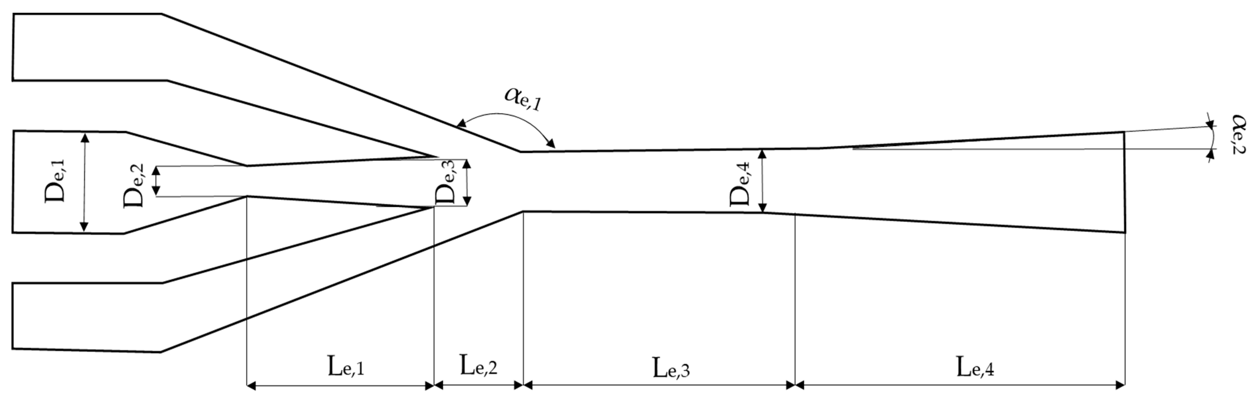
In the following sections, the jet ejector used for this study will be defined first, as well as the conditions under which it will be studied, the CFD software used for the calculation, and the details of the implemented model.

2.1. Jet Ejector

As the geometry of the jet ejector plays an important role in determining its performance, this study focuses on a particular jet ejector designed throughout previous work and is intended to work in a jet ejector refrigeration cycle [18]. Figure 1 illustrates an exemplary geometry of the fixed jet ejector, while

Table 1. The measured ejector’s dimensions, in regard to Figure 1.

De,1 [mm]	De,2 [mm]	De,3 [mm]	De,4 [mm]	Le,1 [mm]	Le,2 [mm]	Le,3 [mm]	Le,4 [mm]	αe,1 [°]	αe,2 [°]
15.194	2.252	3.1978	5.8862	11.01	4.4926	58.12	110.78	159.85	21.8
primary inlet diameter	primary inlet throat diameter	throat diameter	mixing chamber diameter	primary inlet length	junction length	mixing chamber length	diffuser length	angle of secondary inlet entrance	angle of diffuser divergence

summarizes the main geometric parameters of the considered ejector, which are schematically represented in the sketch in Figure 1.

Figure 2 represents the axisymmetric shape of the analyzed jet ejector, designed for refrigeration applications. This ejector was designed to use the refrigerant fluid R1234yf as the working fluid. Additionally,

Table 2. The design conditions of the used jet ejector.

Symbol	Name	Value	Unit
${\mathit{T}}_{\mathit{p}}$	Temp. at primary inlet	362.85	K
${\mathit{T}}_{\mathit{s}}$	Temp. at secondary inlet	273.15	K
${\mathit{p}}_{\mathit{p}}$	Pressure at primary inlet	30.6	bar
${\mathit{p}}_{\mathit{s}}$	Pressure at a secondary inlet	3.2	bar
${\mathit{p}}_{\mathit{o}\mathit{u}\mathit{t}}$	Pressure at outlet	10.7	bar

shows the specific boundary conditions used for its design [18].

The working map used to define the jet ejector’s performance is usually represented by means of a group of characteristic curves, which represents the operating pressures expressed as pressure ratios (${\pi }_{sp}=p_s/p_p$ and ${\pi }_{op}=p_{out}/p_p$) together with the entrainment ratio of the mass flows ($\omega ={\dot{m}}_s/{\dot{m}}_p$). These dimensionless parameters are used to create a working map of the ejector, which graphically and dimensionlessly represents the behavior of the device under different working conditions (see Figure 3).

In Figure 3, the solid lines connect the points with the same π_sp, represented on the ω vs π_op graph. The specific position of these lines depends on the values of π_sp, with higher or lower placements corresponding to its value. When operating a jet ejector under constant inlet temperatures, varying the pressures alone produces predictable results, as observed in the performance maps. Specifically, the relationship between ω and π_op follows a characteristic pattern. It typically begins with a horizontal linear segment (critical zone), when the two flows, primary and secondary flows, are blocked followed by a linear decline at a constant angle (subcritical zone). The dotted line connects the points of transitions from the critical to subcritical modes (critical points). For 3D representation, the plane connecting critical points (*) draws the best operation plane, as at these points are where maximum entrainment ratios ($\omega$) are obtained together with maximum outlet pressure ratios (π_op). At the bottom of the figure, where the entrainment ratios become negative, the reversed secondary flow causes the ejector to be inoperative (backflow operation).

2.2. Software and Modeling Approach

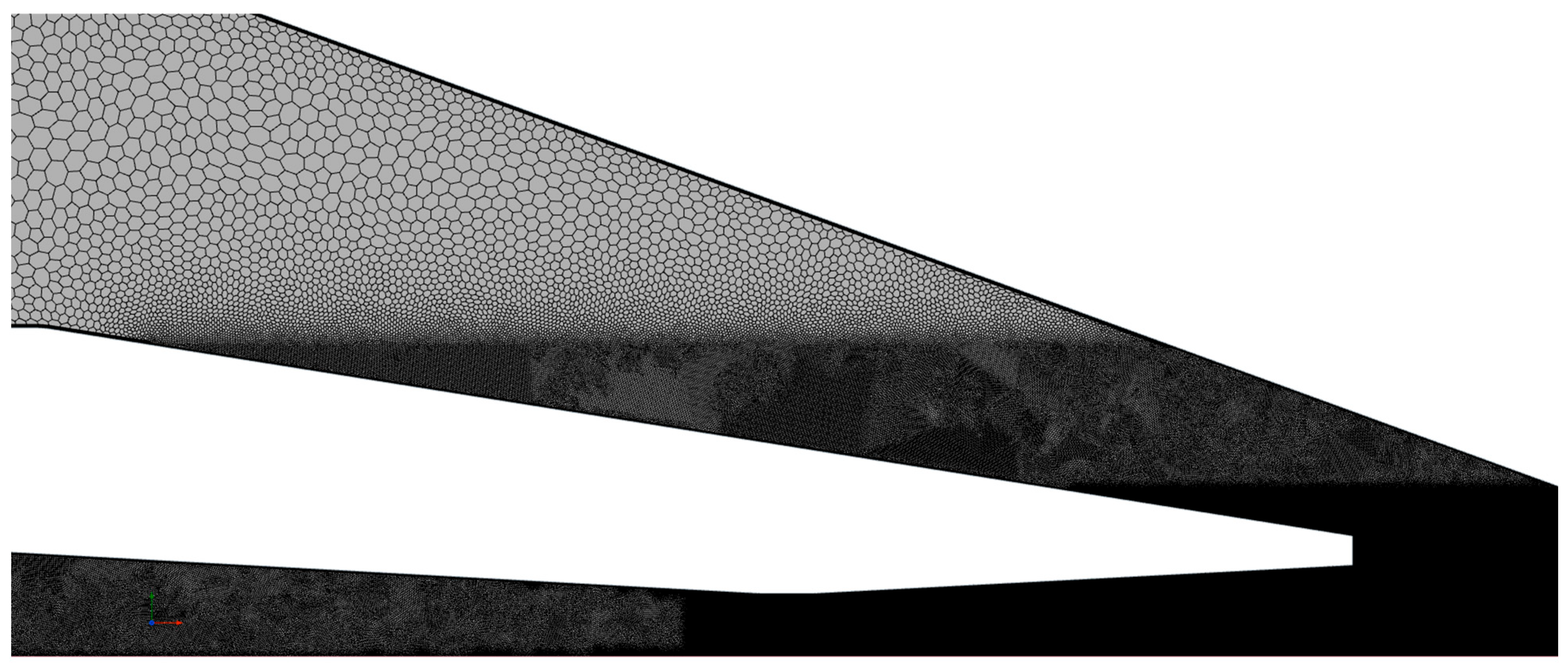
The calculation of the jet ejector model is achieved using Star CCM+ software, version 18.06.007. Geometry has been represented in the 2D axisymmetric configuration. It is a common technique for shortening the calculation time [19,20]. The ideal gas assumption has been used to simplify this study. It is a simplification present in the literature [21], which is shown to provide reliable results [22].

The chosen solver was the steady density-based coupled implicit available in Star CCM+, since it is more appropriate for highly compressible flows. The discretization of the convective term was a 3rd order MUSCL (Monotonic Upstream-centered Scheme for Conservation Laws). This high-order scheme leads to a better description of the shock wave discontinuities without oscillations of the solution thanks to the flux limiters.

In the current state-of-the-art literature, no definitive consensus exists on the most suitable turbulence modeling for jet ejector simulations. When conducting complex simulations, a balance must always be struck between computational efficiency and accuracy. Various studies have analyzed different solvers, each with their own advantages. For instance, Gagan et al. [23] found that the k-ε model was best suited for capturing shockwaves, while Singer [24] argued that the RSM (Reynolds Stress Model) was more appropriate. Both studies, however, also identified the k-ω model as one of the best-performing options.

Each approach to turbulence modeling has distinct strengths depending on the simulation’s focus. The RSM is particularly effective for capturing anisotropic turbulence in the mixing layers but is computationally expensive due to its five-equation framework. The k-ε model, on the other hand, captures better wall friction effects and internal duct flows.

Li et al. [25] conducted a study comparing the k-ε and k-ω models, demonstrating that both provided similar levels of accuracy, aligning well with experimental results within the desired error range. Other studies support the use of the k-ω solver. The results from Mazzelli et al. [26] show that the k-ω SST (shear stress transport) turbulence model performs better than the other models in predicting the flow behavior of a supersonic air ejector, especially under different operating conditions. They have found that although k-ε models are more accurate at low motive pressures, they are less reliable overall. The k-ω SST model stood out because it handled near-wall effects, shock interactions, and recirculation zones more accurately, and those are key factors in supersonic ejector flows. Although global parameters, like mass flow rates and entrainment ratios, do not vary much between models, those studies have found that k-ω SST model provides more accurate local flow predictions, particularly in off-design conditions.

In our simulations, we prioritized precision, yet we also needed to manage a significant number of computational cells. Given these considerations and taking into account the relevance of the mixing layers in the modeling of the ejectors, we selected the k-ω solver, as used in Mazzelli et al.’s study and confirmed by the work of Li et al., to achieve a balance between accuracy and computational feasibility.

Some of the fluids can be found in the Star CCM library as presets for simulations, but this is not the case for the refrigerant R1234yf (2,3,3,3-Tetrafluoropropene). To represent it as an ideal gas, we fed the software with the requested values specific to the fluid. In this study, the thermophysical properties of R1234yf were obtained from the CoolProp open access database and were used as constant values to simulate it as an ideal gas. This follows the constant property approach, where transport and thermodynamic properties remain fixed regardless of temperature or pressure variations, providing a simplified thermophysical model. Namely, the dynamic viscosity has been set to 1.4563 × 10⁻⁵ Pa·s, while the molecular weight is 114.04159 kg/kmol. The specific heat capacity has been assigned a value of 955.7632 J/kg·K, and the thermal conductivity has been set to 0.01797096 W/m·K. Additionally, the turbulent Prandtl number has been fixed at 1.062292.

2.3. Mesh

A mesh sensitivity study has been conducted. The governing parameter for this study was the entrainment ratio, which is a common approach used, for example, by Elmore et al. [27], and the meshes were compared based on the criteria of a number of cells and the value of y+. CFD use a non-dimensional wall distance to describe how close the first grid point—cell center—is to a wall in terms of viscous effects. It helps determine the resolution of the boundary layer near the wall and whether the mesh is fine enough to capture wall-bounded flow phenomena accurately. To define the y+ parameter the following formula is used

$$y^{+}={\displaystyle \frac{y{u}_T}{\nu }}$$

(1)

where $y$ is the distance from the wall to the center of the first computational cell, and $u_{\mathrm{T}}$ is the friction velocity, calculated from the wall shear stress divided by density:

$$u_{\mathrm{T}}=\sqrt{{\displaystyle \frac{{\tau }_w}{\rho }}}$$

(2)

where $\nu$ is the kinematic viscosity of the fluid [28].

Since in our calculations we have wall cells with very low y+ values together with others with higher values, we have selected the “All y+ Wall Treatment” option available in StarCCM+ that blends wall functions for those cells with high y+ values with a low Reynolds treatment for low y+ values. This strategy gives reasonable results for y+ values in the buffer zone (1 < y+ < 30).

The starting case consisted of 16,274 cells in the 2D, axisymmetric geometry. The prism layer mesh was used with geometric progression, stretch factor distribution mode, and a gap fill of 25%.

While the y+ factor is a common criterion for assessing mesh quality, jet ejector studies require a more nuanced approach. In this case, the entrainment ratio—defining the mixing of flows—was the primary indicator, while the y+ factor played a secondary role. This mainly applies to near-wall conditions, but in our case, the key objective was to accurately represent both flow mixing and wall friction effects, which guided the mesh selection.

To conduct the mesh sensitivity study, the number of cells in the initial reference case was progressively increased until stability was observed in the studied variable (entrainment ratio, ω). Figure 4 presents a comparison of entrainment ratios as a function of the number of cells for each case. The corresponding numerical results are detailed in

Table 3. Comparison of different meshes at one working point.

Mesh Version Case Number	Entrainment Ratio	Number of Cells	Max. y+
1	1.146127	16,274	500
2	1.146135	16,274	500
3	1.166865	103,191	160
4	1.175862	214,554	240
5	1.178889	568,805	8.5
6	1.185003	1,625,678	45
7	1.172905	2,910,279	55
8	1.176702	3,475,381	20
9	1.176702	3,608,526	20
10	1.176702	3,785,626	20
11	1.176702	3,985,944	20

, where case no. 1 represents the starting mesh, and subsequent cases show progressively refined versions. The last four cases, featuring the densest meshes, yielded similar entrainment ratio results, indicating convergence.

To balance accuracy with reasonable computation time, case no. 8—comprising 3,475,381 cells—was selected as the reference mesh for this study and is referred to as refined.

The refined mesh features a notably high resolution, with over 3,470,000 cells. This is significantly greater than the cell counts in other studies on supersonic jet ejectors, where 2D axisymmetric models can range from 20,300 cells [29] to 330,000 cells [24], and even than detailed 3D models, such as those by Hou et al. (982,362 cells) [30]. While this resolution increases computational demands, it improves simulation accuracy. Using a less refined mesh in CFD simulations can lead to several issues that compromise the accuracy of results. One major consequence is the inaccuracy in capturing Mach number distributions. Insufficient mesh refinement can also produce artificial shock waves or “numerical artifacts” that do not physically exist, thereby distorting the shock wave structure and interactions. In this type of jet ejector, the primary flow reaches supersonic conditions, producing a discharge jet with a set of oblique shock waves and expansion waves. The defined mesh must be sufficiently dense to allow the correct representation of these shock waves and to accurately locate them in the ejector.

As mentioned earlier, the literature commonly employs meshes with lower resolutions, typically containing 20,000 to 300,000 cells [24,29]. To evaluate the impact of mesh refinement on the accuracy of the simulations, we compared the highly refined mesh with a coarser one that aligns with conventional approaches. This comparison aimed to assess precision differences and justify the high cell count used in case no. 8 (Table 3). For this comparative analysis, an additional mesh case was selected to represent lower-resolution meshes. Specifically, case no. 3 from Table 3 was chosen, as it was the first to show a significant reduction in the y+ number, an entrainment ratio close to the final achieved value, and a moderate cell count within the same order of magnitude as those reported in the literature. This mesh is a generic, structured grid applied to the entire ejector geometry, generated using a polygonal mesh combined with a prism layer meshing.

The mesh is a high-quality, two-dimensional structure confined to the xy-plane, with spatial dimensions of 0.34551 m in the x-direction and 0.01500 m in the y-direction. It consists of over 100,000 cells and maintains a mesh quality of 0.05, with a base size of 0.001 m. The mesh includes eight prism layers with a stretch factor of 1.1, where the minimum thickness is set at 10% of the base size, and the total prism layer thickness is also 10%. This coarser mesh version used for result comparison is referred to as coarser in the analysis.

The same generic mesh has been used as a base for the refined case. Whereas some parts of the ejector where the flow is in subsonic conditions will not have shock waves and will not need denser meshing (subsonic flow will take place at the entrance of the primary and secondary flows and at the end of the diffuser), in the divergent part of the nozzle of the primary flow and in the mixing zone of the two flows, the flow will be in supersonic conditions and will require a more refined meshing [15].

To improve accuracy in areas where the flow is supersonic, two zones were defined where more precision was needed with the calculations. Figure 5 shows these two zones designated with the names Block I and Block II.

These rectangular zones with custom control differ by the base cell size and prism layer thickness. Additionally, to ensure the accurate resolution of shock waves and steep pressure gradients, a dynamic refinement strategy was implemented using a field function-based refinement approach. The refinement was governed by the magnitude of the pressure gradient, defined as mag(∇P), through the conditional expression, shown in Equation (3), where each set of cases has been studied to define the ranges of pressure gradients appearing and the refinement function was updated.

$$\mathrm{Refinement} \mathrm{Size}=\left\{\begin{array}{ll}1\times {10}^{-7}& \mathrm{if}\mathrm{m}\mathrm{a}\mathrm{g}(\nabla P)>5\times {10}^{10},\\ 1\times {10}^{-6}& \mathrm{if}\mathrm{m}\mathrm{a}\mathrm{g}(\nabla P)>5\times {10}^9,\\ 1\times {10}^{-5}& \mathrm{if}\mathrm{m}\mathrm{a}\mathrm{g}(\nabla P)>5\times {10}^8,\\ 1.2\cdot {\mathrm{Volume}}^{1/3}& \mathrm{otherwise}.\end{array}\right.$$

(3)

As Equation (3) shows, if the pressure gradient, mag(∇P), exceeds $5\times {10}^{10}$, the refinement base cell size (rbcs) is set to $1\times {10}^{-7}$, providing the highest level of refinement. For regions with a gradient greater than $5\times {10}^9$, an rbcs of $1\times {10}^{-6}$ is applied, while for gradients exceeding $5\times {10}^8$, the rbcs is $1\times {10}^{-5}$. In all other areas, where pressure variations are more gradual, the refinement size is determined by the $1.2\cdot {\mathrm{Volume}}^{1/3}$. This term estimates a characteristic length scale of the mesh cell, where ${\mathrm{Volume}}^{1/3}$ provides an approximate side length, and the factor 1.2 ensures a moderate refinement level.

These procedures resulted in a mesh diversity, which can be spotted in Figure 6.

This approach, combining the generic mesh with two additional zones for the refinement, and the adaptive refinement function ensured that areas with significant pressure gradients received finer mesh resolution, enabling precise capturing of shock wave structures. By dynamically updating the mesh with each iteration, the meshing approach remained responsive to changes in the solution field, enhancing overall accuracy and computational efficiency. The number of cells is therefore dependent on the case, as they are reactive to changes in local pressure.

2.4. Governing Equations

In STAR-CCM+, the governing equations used for simulations are based on the Navier–Stokes equations, which describe the motion of fluid substances. These equations consist of the continuity equation (mass conservation), the momentum equation (Newton’s second law for fluids), and the energy equation (first law of thermodynamics). The solver also incorporates turbulence and viscosity models (k-ω). Additionally, transport equations are solved for scalar quantities, like spacious concentration and temperature, enabling simulations of multiphase flows. The software uses the finite volume method to discretize these governing equations and transform them into algebra that can be solved numerically [31]. For this case, the coupled implicit solver and the GammaReTheta transitions were also applied.

2.5. Simulation Campaign

The simulation campaign was multistage. It consisted of first creating a line of the working map (π_sp = 0.26) of the considered jet ejector with constant values for primary pressure (p_p = 35 bars), primary temperature (T_p = 380 K), secondary temperature (T_s = 313 K), and p_out changing. The values of π_op were adjusted throughout the simulations in order to complete the line of the jet ejector working map. This line of the working map has been plotted by using two meshes—coarser and refined.

The second stage was to then repeat the calculation of the π_sp = 0.26 line with the refined mesh, while changing the inlet temperatures (T_p and T_s) proportionally in order to determine the sensibility of the jet ejector performance to these changes. A scaling coefficient ζ is introduced to alter both inlet temperatures while maintaining a controlled variation systematically. The values used for this coefficient and temperatures are expressed in

Table 4. Inlet temperatures values according to ζ coefficients.

Default T Values	ζ’ = 1.1 [/]	ζ” = 1.2 [/]
$T_p$ = 380 K	$T_p’$ = 418 K	$T_p”$ = 456 K
$T_s$ = 313 K	$T_s’$ = 344.3 K	$T_s”$ = 375.6 K

. The chosen ζ values assured the working fluid to be in a supercritical phase and that the results make physical sense.

The last stage of the work has as an objective to change only the primary temperature (T_p). To do so, we conducted the third part of the analysis, multiplying the T_p by a factor of 1.2 (so T_p = 456 K), but keeping the T_s constant (T_s = 313 K).

3. Results

The following sections show the results of the three studies carried out. In Section 3.1, the comparison of the results obtained with the coarser and refined mesh is shown. In Section 3.2, the comparison of the results obtained with the refined mesh by proportionally varying both inlet temperatures is shown, and in Section 3.3 the comparison of the results of the refined mesh by varying only the inlet temperature of the primary flow is shown.

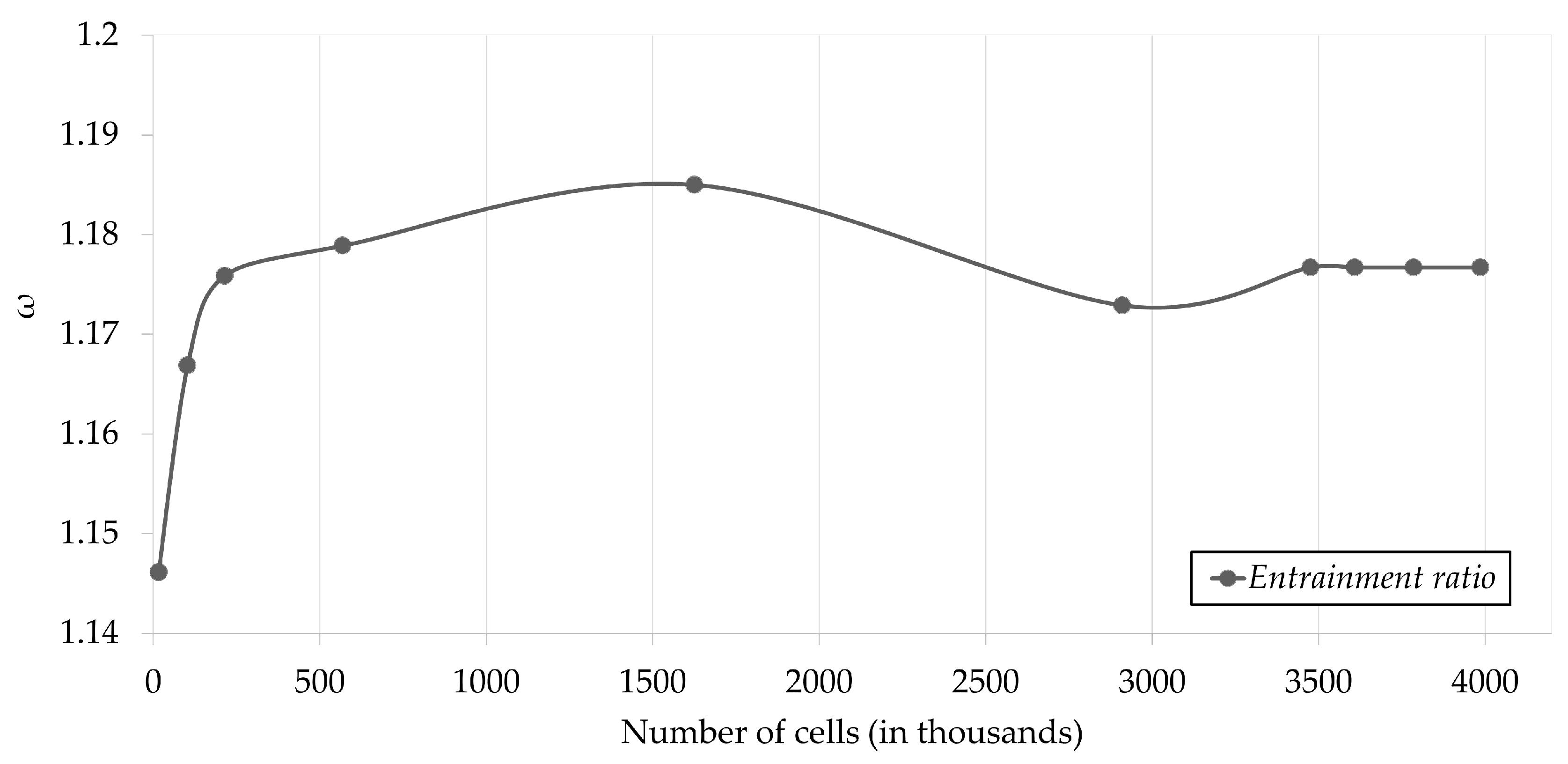
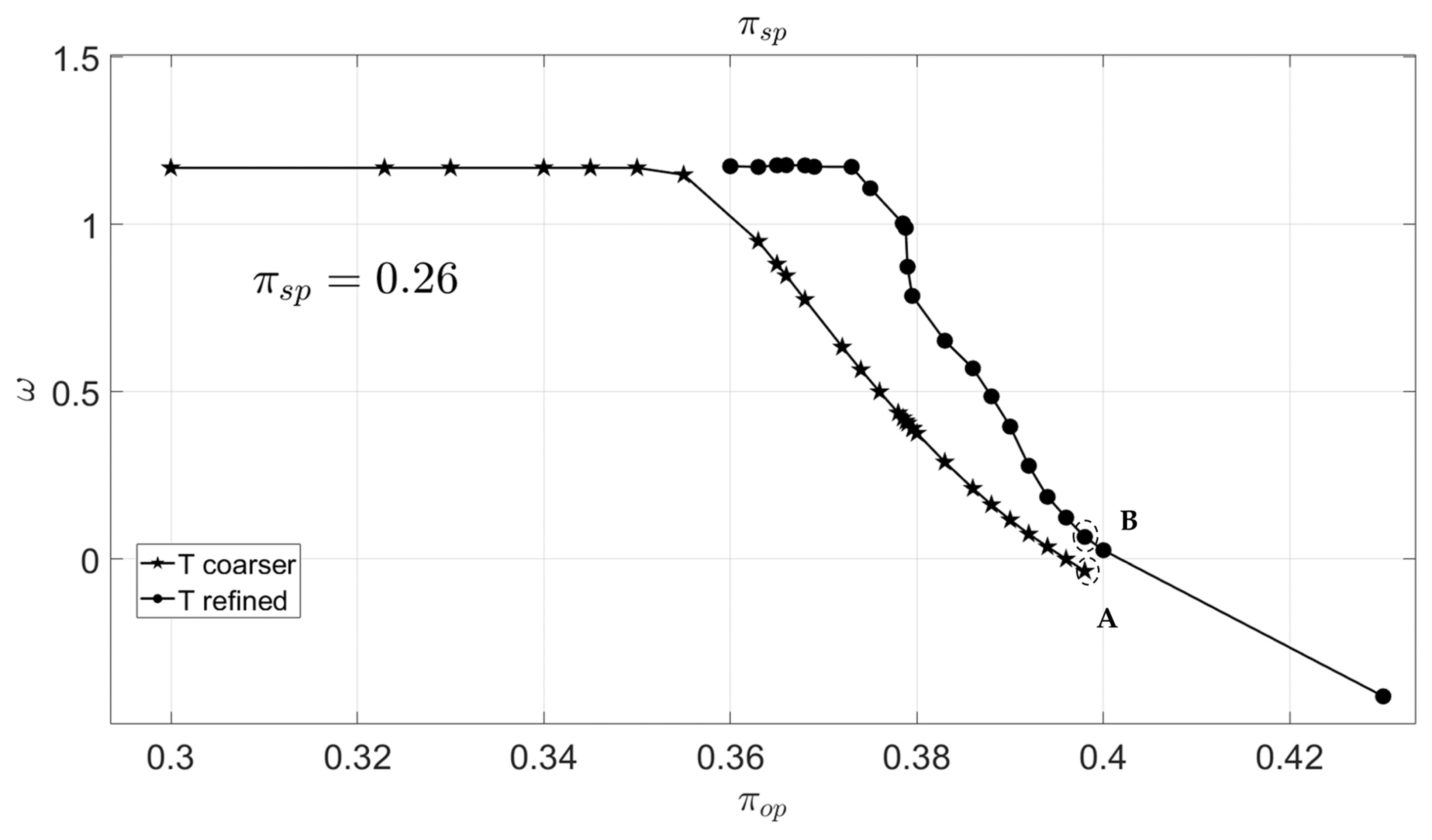
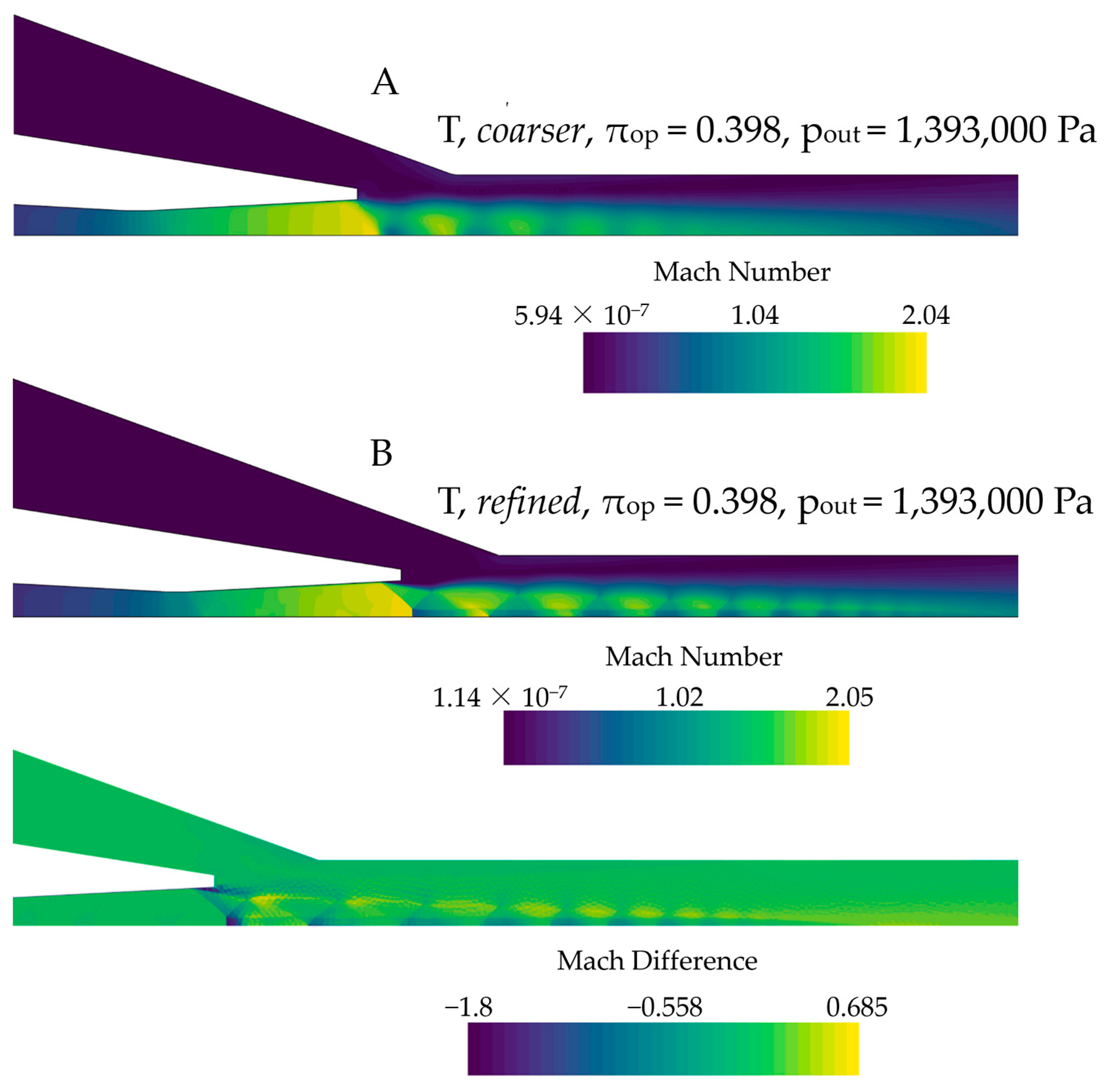
3.1. Analysis of Different Meshes—Coarser and Refined Meshes

This part of the study analyzes the considered constant boundary values (p_p = 35 bars, T_p = 380 K, T_s = 313 K, and π_sp = 0.26) and the two meshes. The refined mesh used in this study is the mesh version of case no. 8 from Table 3, which features a notably high resolution. It is compared with the results obtained with the coarser mesh (case no. 3 from Table 3) to see the differences between the “traditional meshing” (with cell numbers similar to our coarser mesh) with the high-resolution meshing proposed in this work (refined).

As can be seen in the graph in Figure 7, the results obtained with the coarser mesh and the adaptive refined mesh differ. The distortions can be seen in the comparison of Mach number distributions of coarser and refined meshes, illustrated in Figure 8 below, which highlights the impact on the Mach number scene representation with the different mesh precisions, coarser on the top and refined on the bottom. These inaccuracies result from the inability of the coarser mesh to resolve steep gradients in pressure, temperature, or velocity accurately, especially near shock regions and boundaries. Additionally, it can lead to unclear or inconsistent readings of flow behaviors, such as turbulence levels or boundary layer separation [32].

Similarly, the larger inaccuracies while using the coarser mesh observed in Figure 8 produce differences in the mass flow results (affecting entrainment ratios). These differences in entrainment ratios translate into different representations of the working map line. Figure 7 shows the comparison between the π_sp = 0.26 pressure ratio lines obtained using the coarser (stars) and the refined (circles) meshes. In the graph, we can see that the maximum entrainment ratio (critical conditions) in both cases is the same (at ω = 1.17). However, the subcritical zone for the coarser mesh starts earlier, at π_op = 0.355, while for the refined mesh the transition occurs at π_op = 0.375. The lines get closer to each other towards the negative entrainment ratio values as the negative slope in the refined mesh is higher than in the coarser case. Furthermore, this negative slope (subcritical zone) is more constant in the case of the coarser mesh than in the case of the refined mesh, where a certain wavy shape can be observed in this negative slope. As shown in the figure, a refined mesh shows details of the ejector behavior that cannot be observed with coarser meshes. It shows that the better-refined mesh is able to better catch the intricate shapes of the oblique shock waves and how they affect the entrainment ratios obtained.

In order to observe, in more detail, the difference in the obtained results between the coarser mesh and the refined mesh, two cases have been selected and are represented in Figure 7 as cases A and B. These two cases are close cases with similar pressure ratios, and the comparison of the Mach number distribution in both cases can be seen in Figure 8.

In the upper part of Figure 8, the Mach number distribution is shown for both cases, while the lower part presents the Mach number difference between scenes at points A and B (from Figure 7). In these scenes, the improvement in results when using the refined mesh can be observed, especially in the representations of the oblique shock waves. In the lower part of the figure, the differences in Mach number distributions and values between the scenes for cases A and B are represented. It can be observed that the most important differences in the results occur throughout the supersonic jet, especially in the area with higher Mach number values. These differences in the distribution of shock waves in the jet cause slight discrepancies in the results and produce the differences in the entrainment ratios observed in Figure 7.

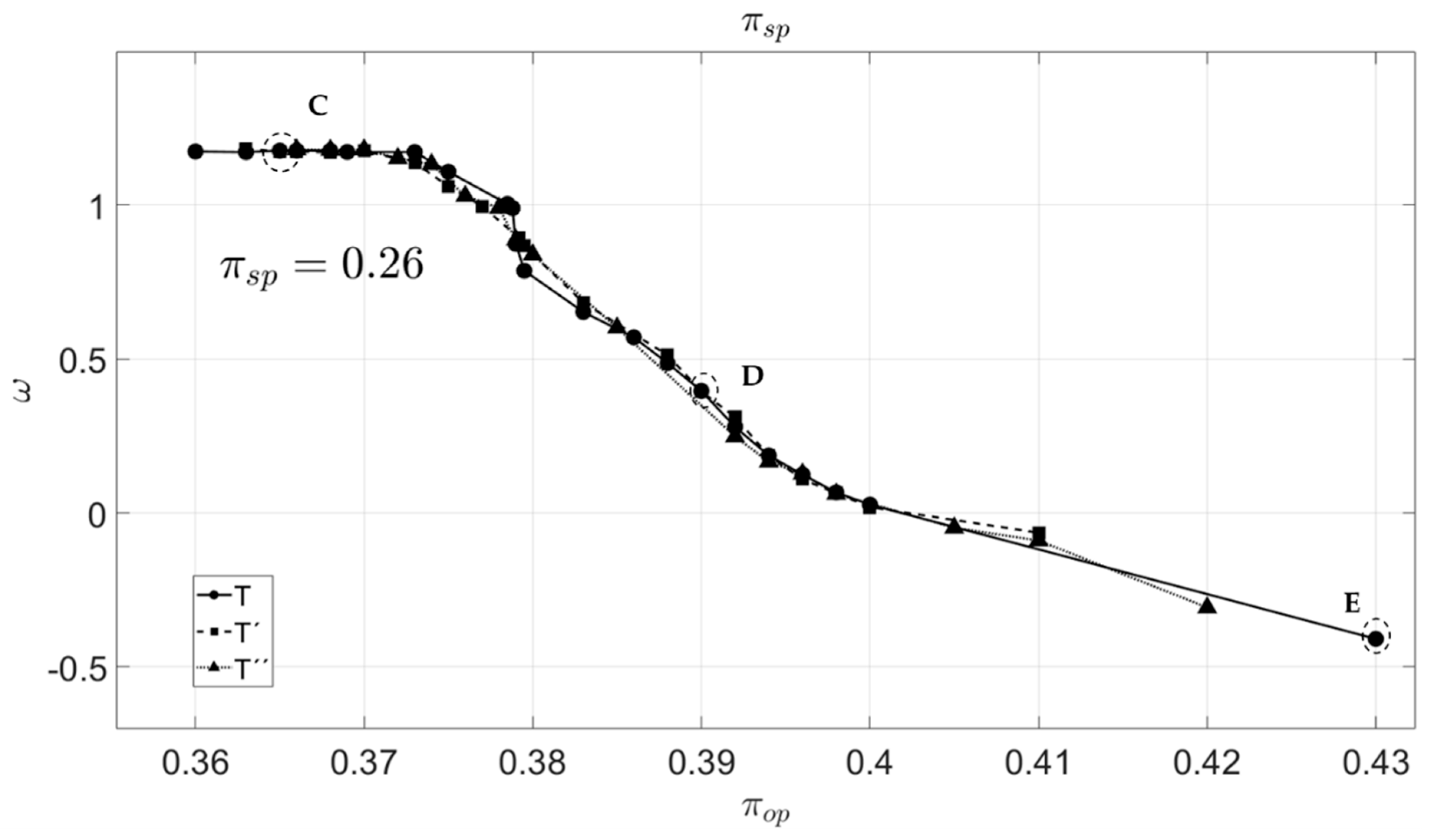
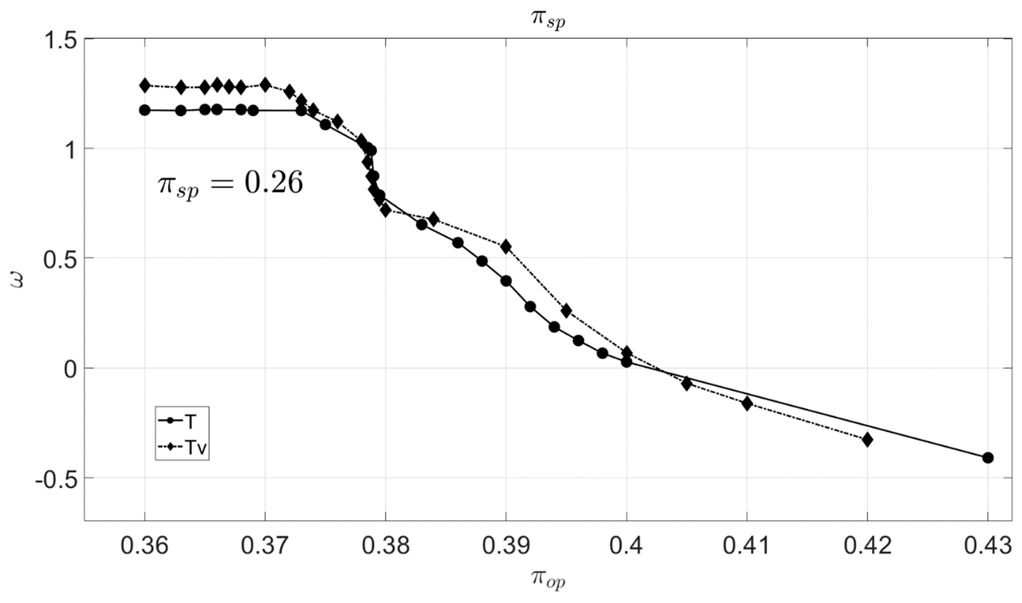
3.2. Analysis for Temperature Changes Using Refined Mesh

This case depicts the three temperatures variations, according to the ζ coefficient introduced in Table 4 and calculated using the refined mesh. As defined in Table 4, in this study three temperature levels will be compared at the ejector inlets: the T case where the reference temperatures at the inlets are imposed (T_p = 380 K, T_s = 313 K); the T’ case where these temperatures are imposed multiplied by a factor of 1.1, and the T” case where the temperatures are multiplied by 1.2.

Figure 9 shows the comparison of the line π_sp = 0.26 for the three temperature levels. By increasing the inlet temperatures at both inlets proportionally, the dimensionless values that determine the ejector operation do not vary and result in a similar line of behavior on the ejector map. As can be seen in the graph below, the three lines coincide in the critical zone, as well as in the critical point and in the subcritical zone. In all three cases, the same oscillating behaviors of the subcritical zone and the variability of its negative slope are observed. This repeatability in the results, reproducing the intricate wavy shape of the ejector behavior in the subcritical zone, gives a clear demonstration of the precision of the refined mesh.

In order to compare, in detail, the obtained results at the three different regions (critical, subcritical, and backflow) at one temperature, points C, D, and E of Figure 9 have been marked for a more detailed analysis. Figure 10 shows the Mach number distribution in the ejector for the three chosen points, C, D, and E, for the T temperature. In this figure, to facilitate the visualization of the flow under supersonic conditions, only the areas where the Mach number is greater than one have been represented on the color scale. As can be seen, the shockwave distribution follows the expected trend. Moreover, all cases with different temperatures revealed the same tendency when they change from the critical, to the subcritical, to the backflow zones.

In Figure 10, the top snap shows the Mach number scene for the critical conditions (point C). We can see that the flow is double chocked because in the mixing zone, where the primary and secondary flows mix, the supersonic behavior of the flow occupies the entire cross-section, blocking the pass of both flows. At the outlet of the primary nozzle, the first oblique shock wave appears producing a Mach disk in the axis zone of the ejector. It is then followed by a chain of diamond oblique shockwaves, continuing toward the mixing chamber. Later, the amplitude of the waves diminishes, to eventually disappear around the entrance of the diffuser. The figure also shows the first part of the jet where the walls of the duct affect its shape and produce the aforementioned blockage of the entire cross-section of the ejector.

The second scene (point D) in the middle, represents the subcritical conditions. In this case, we can see that only the primary flow is choked, and the secondary flow has a passage close to the walls in subsonic conditions. In this case, the jet length is lower than the previous case and the waves disappear around the middle of the mixing zone.

The bottom snap (point E) represents the backflow condition’s Mach number scene. In this case, the chain of oblique shockwaves is very short and ends in the first part of the mixing zone. This smaller jet produces an increase in the secondary flow section pass and causes the return of the flow near the ejector wall due to the pressure difference between the ejector outlet and the secondary inlet. When this backflow through the ejector periphery is greater than the flow entrained through the center of the ejector, the backflow conditions of case E occur.

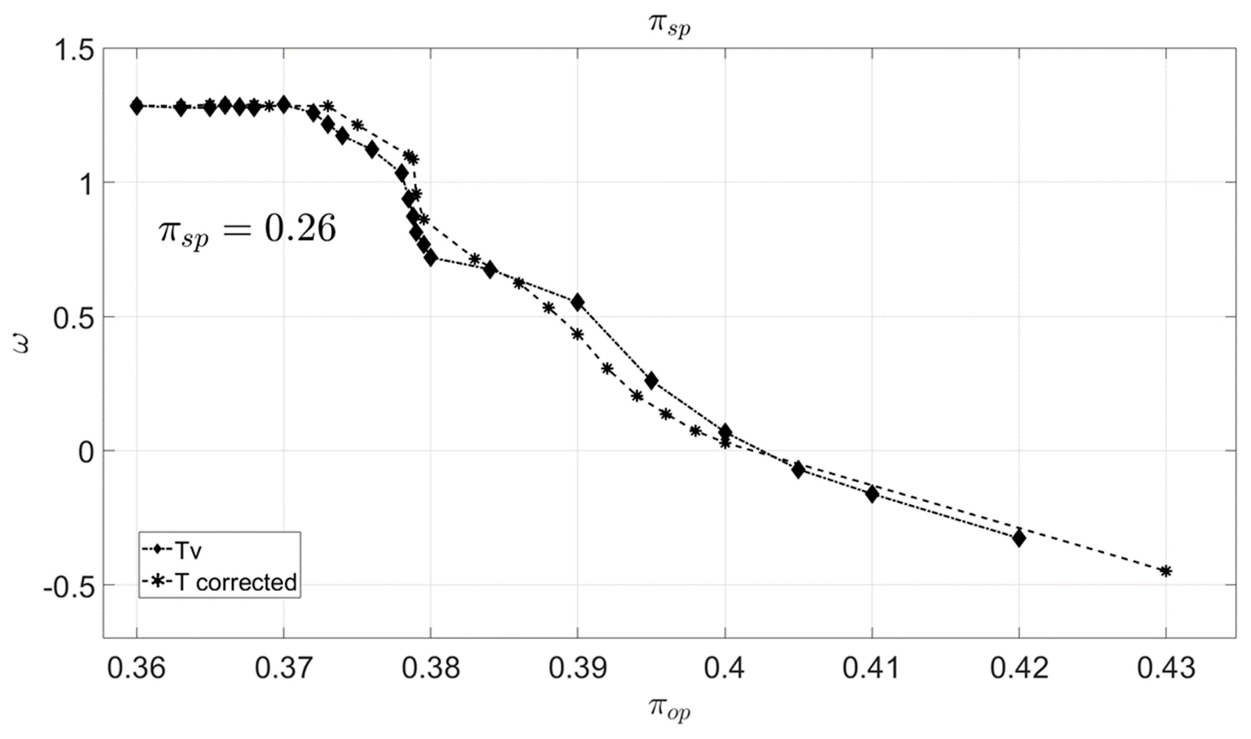
3.3. The Analysis for the Primary Temperature Variations Using the Refined Mesh

The third study has the objective to analyze the differences when only the primary temperature changes and using the refined mesh. The graph in Figure 11 shows the lines for the default primary temperature (T_p = 380 K), marked as “T” and represented with circular markers, and a case with this temperature increased by a factor of 1.2 (T_p = 456 K), marked as “Tv”, with diamond shaped markers. In this case, by increasing only the temperature of the primary flow, only the stagnation conditions in the primary inlet are changed, without affecting the conditions at the secondary inlet, which remain constant. As can be seen in the figure, this produces an increase in the entrainment capacity of the primary flow (entrainment ratio) when the ejector is working in critical conditions. These differences between the two cases are maintained throughout the critical behavior zone.

The difference in the entrainment ratio when the primary temperature increases by a factor of 1.2 is a variation from 1.17 to 1.28 in critical conditions. When dimensionless maps are used, the values obtained must be corrected with the temperatures and pressures used as reference. In this case, to correct the mass flow rates used in the map, they must be corrected with the square root of the temperature variation. In our case, the observed increase in the entrainment ratio coincides with the square root of the variation in the inlet primary temperatures, since $\sqrt{1.2}·1.17=1.28$. However, when they are changed to subcritical conditions, the behavior in both cases is very similar, and no significant differences are observed.

To check this, we corrected the results obtained from the case with the default primary temperature and compared it with the “Tv” results (a case with a primary inlet temperature increased by a factor of 1.2).

We can calculate the corrected entrainment ratio, as indicated in Equation (4):

$${\mathsf{\omega }}^{\ast }={\displaystyle \frac{\dot{m_s^{\ast }}}{\dot{m_p^{\ast }}}}$$

(4)

And as the $\dot{m_s^{\ast }}=const.$, we can focus on calculating the $\dot{m_p^{*}}$ in the primary inlet as follows Equation (5):

$$\dot{m_p^{*}}={\displaystyle \frac{\sqrt{\raisebox{1ex}{$T_v$}\!\left/ \!\raisebox{-1ex}{$T$}\right.}}{\raisebox{1ex}{$p_v$}\!\left/ \!\raisebox{-1ex}{$p$}\right.}}$$

(5)

In our case, the pressures remain constant, and the proportions of primary temperatures were namely 1.2; therefore, we obtained the “T corrected” entrainment ratio results as calculated in Equation (6):

$${\mathsf{\omega }}^{\ast }=\sqrt{1.2}·{\mathsf{\omega }}_v$$

(6)

Figure 12 below presents the graph of those plotted results, with the “Tv” marked with diamonds and “T corrected” with star symbols.

As can be seen, the curves fit. The critical operations zone values for the entrainment ratio overlap. After entering the subcritical operations zone, although the lines fluctuate, both cases seem to follow the same patterns. Then, towards the backflow operations regime they get closer again.

4. Conclusions

This paper studies the differences observed when using a coarse mesh and a refined mesh in CFD studies of jet ejectors. Traditionally, the studies found in the literature use rather coarse meshes, with a very limited number of cells.

Today, the computational capacity available for these calculations has greatly increased and allows for the use of more precise meshes. In this paper, the use of one of these coarse meshes is compared with a refined mesh. This refined mesh is also adaptive and changes locally depending on the pressure gradients introduced by the shock waves, thus improving the accuracy of the calculation in those areas that require it. The results obtained from this comparison show significant differences in predicting the jet ejector behavior. These differences do not affect the jet ejector behavior under critical conditions, but they do affect the critical point, where the transition between critical and subcritical behavior occurs, and the behavior under subcritical conditions.

This study shows that with the coarser mesh, the entrainment ratios obtained in the subcritical zone present a more constant behavior in the downward slope of the ejector work map. On the other hand, for the more precise refined mesh, the results show a more detailed and intricate behavior with slight variations in the subcritical slope.

The presented approach is one of the possibilities of the meshing strategy. Two different refinements have been applied: block refinement in specific regions and adaptive refinement based on the pressure gradient field function. They were applied sequentially; however, it is possible that using intermediate block refinement in conjunction with pressure gradient refinement could achieve similar results with a lower cell count. Additionally, the further optimization of the block regions and gradient threshold values could enhance the efficiency of the meshing strategy.

In order to evaluate the repeatability of the results with the refined mesh, a study has been carried out by proportionally varying the temperatures at the primary and secondary inlets. In this study, the reference case has been compared with a case where both temperatures have been increased by 10% and another case where they have been increased by 20%. By increasing the two temperatures in the same proportion, the energy of the two flows increases proportionally and, as expected, the results obtained in the three cases are similar, showing the repeatability of the results obtained for the reference case. The distributions of the Mach number inside the ejector have also been compared, observing the differences introduced by the ejector’s behavior under critical, subcritical, and backflow conditions.

Finally, the differences in ejector behavior have been studied when only the temperature of the primary is changed, increasing its value by 20% and leaving the temperature of the secondary constant. In this case, differences are observed since the primary flow increases its energy without changing the energy supplied to the secondary inlet. These differences translate into changes in the jet ejector behavior in the critical zone. However, these differences are smaller in the subcritical zone.

Correcting the ejector map when working with different temperatures can be relevant and must be considered when working with these maps. The publication of these maps while clearly defining all the boundary conditions used to obtain them is essential to be able to perform their proper correction when they are used.

Overall, this study has achieved its intended objectives. The key contribution lies in the sensitivity of the simulations, particularly in the meshing strategy, which has successfully captured effects that remain undetected at the mesh resolutions commonly used in the literature. By refining the meshing approach, we have identified phenomena that standard discretization methods may overlook, underscoring the critical role of mesh sensitivity in numerical analysis. While this work does not provide a definitive solution to the problem, it highlights its complexity and the limitations of conventional meshing techniques, paving the way for further investigation and refinement in future research.

References

1. Elbel, S.; Hrnjak, P. Experimental validation of a prototype ejector designed to reduce throttling losses encountered in transcritical R744 system operation. Int. J. Refrig. 2008, 31, 411–422. [Google Scholar] [CrossRef]
2. Nakagawa, M.; Marasigan, A.R.; Matsukawa, T.; Kurashina, A. Experimental investigation on the effect of mixing length on the performance of two-phase ejector for CO2 refrigeration cycle with and without heat exchanger. Int. J. Refrig. 2011, 34, 1604–1613. [Google Scholar] [CrossRef]
3. Varga, S.; Oliveira, A.; Diaconu, B. Influence of geometrical factors on steam ejector performance- a numerical assessment. Int. J. Refrig. 2009, 32, 1694–1701. [Google Scholar] [CrossRef]
4. Yapici, R.; Ersoy, H.K. Performance characteristics of the ejector refrigeration system based on the constant area ejector f low model. Energy Conv. Manag. 2005, 46, 3117–3135. [Google Scholar] [CrossRef]
5. Godefroy, J.; Boukhanouf, R.; Riffat, S. Design, testing and mathematical modelling of a small-scale CHP and cooling system. Appl. Therm. Eng. 2007, 27, 68–77. [Google Scholar] [CrossRef]
6. Rogdakis, E.D.; Alexis, G.K. Design and parametric investigation of an ejector in an air-conditioning system. Appl. Therm. Eng. 2000, 20, 213–226. [Google Scholar] [CrossRef]
7. Rusly, E.; Aye, L.; Charters, W.W.S.; Ooi, A. CFD analysis of ejector in a combined ejector cooling system. Int. J. Refrig. 2005, 28, 1092–1101. [Google Scholar] [CrossRef]
8. Sriveerakul, T.; Aphornratana, S.; Chunnanond, K. Performance prediction of steam ejector using computational fluid dynamics: Part 2. Flow structure of a steam ejector influenced by operating pressures and geometries. Int. J. Therm. Sci. 2007, 46, 823–833. [Google Scholar] [CrossRef]
9. Keenan, J.H.; Neumann, E.P.; Lustwerk, F. An investigation of ejector design by analysis and experiment. J. Appl. Mech. 1950, 17, 299–309. [Google Scholar] [CrossRef]
10. Bartosiewicz, Y.; Aidoun, Z.; Mercadier, Y. Numerical assessment of ejector operation for refrigeration applications based on CFD. Appl. Therm. Eng. 2006, 26, 604–612. [Google Scholar] [CrossRef]
11. Little, A.B.; Bartosiewicz, Y.; Garimella, S. Visualization and Validation of Ejector Flow Field with Computational and First-Principles Analysis. J. Fluids Eng. 2015, 137, 051107. [Google Scholar] [CrossRef]
12. Cizungu, K.; Mani, A.; Groll, M. Performance comparison of vapour jet refrigeration system with environment friendly working fluids. Appl. Therm. Eng. 2001, 21, 585–598. [Google Scholar] [CrossRef]
13. Chen, Z.; Jin, X.; Dang, C.; Hihara, E. Ejector performance analysis under overall operating conditions considering adjustable nozzle structure. Int. J. Refrig. 2017, 84, 274–286. [Google Scholar] [CrossRef]
14. Haider, M.; Elbel, S. Development of ejector performance map for predicting fixed-geometry two-phase ejector performance for wide range of operating conditions. Int. J. Refrig. 2021, 128, 232–241. [Google Scholar] [CrossRef]
15. Zhu, Y.; Jiang, P. Experimental and analytical studies on the shock wave length in convergent and convergent–divergent nozzle ejectors. Energy Convers. Manag. 2014, 88, 907–914. [Google Scholar] [CrossRef]
16. Han, Y.; Wang, X.; Yuen, A.C.Y.; Li, A.; Guo, L.; Yeoh, G.H.; Tu, J. Characterization of choking flow behaviors inside steam ejectors based on the ejector refrigeration system. Int. J. Refrig. 2020, 113, 296–307. [Google Scholar] [CrossRef]
17. Allouche, Y.; Bouden, C.; Varga, S. A CFD analysis of the flow structure inside a steam ejector to identify the suitable experimental operating conditions for a solar-driven refrigeration system. Int. J. Refrig. 2014, 39, 186–195. [Google Scholar] [CrossRef]
18. Galindo, J.; Gil, A.; Dolz, V.; Ponce-Mora, A. Numerical Optimization of an Ejector for Waste Heat Recovery Used to Cool Down the Intake Air in an Internal Combustion Engine. J. Therm. Sci. Eng. Appl. 2020, 12, 051024. [Google Scholar] [CrossRef]
19. Han, Y.; Wang, X.; Sun, H.; Zhang, G.; Guo, L.; Tu, J. CFD simulation on the boundary layer separation in the steam ejector and its influence on the pumping performance. Energy 2019, 167, 469–483. [Google Scholar] [CrossRef]
20. Pianthong, K.; Sheehanam, W.; Behnia, M.; Sriveerakul, T.; Aphornratana, S. Investigation and improvement of ejector refrigeration system using computational fluid dynamics technique. Energy Conv. Manag. 2007, 48, 2556–2564. [Google Scholar] [CrossRef]
21. Tang, Y.; Liu, Z.; Li, Y.; Yang, N.; Wan, Y.; Chua, K.J. A double-choking theory as an explanation of the evolution laws of ejector performance with various operational and geometrical parameters. Energy Conv. Manag. 2020, 206, 112499. [Google Scholar] [CrossRef]
22. Ruangtrakoon, N.; Aphornratana, S. Design of steam ejector in a refrigeration application based on thermodynamic performance analysis. Sustain. Energy Technol. Assess. 2019, 31, 369–382. [Google Scholar] [CrossRef]
23. Gagan, J.; Smierciew, K.; Butrymowicz, D.; Karwacki, J. Comperative study of turbulence models in applications to gas ejectors. Int. J. Therm. Sci. 2013, 78, 9–15. [Google Scholar] [CrossRef]
24. Singer, G.; Pinsker, R.; Stelzer, M.; Aggarwal, M.; Pertl, P.; Trattner, A. Ejector validation in proton exchange membrane fuel cells: A comparison of turbulence models in computational fluid dynamics (CFD) with experiment. Int. J. Hydrogen Energy 2024, 61, 1405–1416. [Google Scholar] [CrossRef]
25. Li, Y.; Niu, C.; Shen, S.; Mu, X.; Zhang, L. Turbulence model comperative study for complex phenomena in supersonic steam ejectors with double choking mode. Entropy 2022, 24, 1215. [Google Scholar] [CrossRef]
26. Mazzelli, F.; Little, A.B.; Garimella, S.; Bartosiewicz, Y. Computational and experimental analysis of supersonic jet ejector: Turbulence modelling and assessment of ·D effects. Int. J. Heat Fluid Flow. 2015, 56, 305–316. [Google Scholar] [CrossRef]
27. Elmore, E.; Al-Mutairi, K.; Hussain, B.; El-Gizawy, A.S. Development of analytical model for predicting dual-phase ejector performance. In Proceedings of the ASME International Mechanical Engineering Congress and Exposition, Phoenix, AZ, USA, 11–17 November 2016. [Google Scholar] [CrossRef]
28. Siemens Digital Industries Software. Siemens STAR-CCM+ User Guide, version 2021.1. In Adaptive Mesh Refinement for Overset Meshes; Siemens: Munich, Germany, 2021. [Google Scholar]
29. Macia, L.; Castilla, R.; Gámez, P.J. Simulation of ejector for vacuum generation. IOP Conf. Ser. Mater. Sci. Eng. 2019, 659, 012002. [Google Scholar] [CrossRef]
30. Hou, Y.; Chen, F.; Zhang, S.; Chen, W.; Zheng, J.; Chong, D.; Yan, J. Numerical simulation study on the influence of primary nozzle deviation on the steam ejector performance. Int. J. Therm. Sci. 2022, 179, 107633. [Google Scholar] [CrossRef]
31. Gutiérrez Suárez, J.A.; Galeano Urueña, C.H.; Gómez Mejía, A. Adaptive Mesh Refinement Strategies for Cost-Effective Eddy-Resolving Transient Simulations of Spray Dryers. Chem. Eng. 2023, 7, 100. [Google Scholar] [CrossRef]
32. Sehoon, K.; Sejin, K. Experimental Investigation of an Annular Injection Supersonic Ejector. AIAA J. 2006, 44, 1905–1908. [Google Scholar] [CrossRef]
Figure 1. An illustrative drawing showing the location of individual dimensions.
Applsci 15 03880 g001
Figure 2. The actual geometry of the ejector, represented in 2D-axisymmetric shape, with the main variables noted.
Applsci 15 03880 g002
Figure 3. A schematic representation of the working map of an ejector.
Applsci 15 03880 g003
Figure 4. Dependency of entrainment ratio on number of cells.
Applsci 15 03880 g004
Figure 5. The placement of the zones defined for the additional refinement in the refined mesh.
Applsci 15 03880 g005
Figure 6. Zoom on the mesh gradations in refined mesh.
Applsci 15 03880 g006
Figure 7. The lines of πsp = 0.26 for the comparison between the coarser and refined meshes.
Applsci 15 03880 g007
Figure 8. Mach number scenes comparison. On top: Mach number scenes views at consecutive A and B points from Figure 7. On bottom: Mach number differences between both cases.
Applsci 15 03880 g008
Figure 9. The lines of πsp = 0.26 for the temperatures according to Table 4 using the refined mesh.
Applsci 15 03880 g009
Figure 10. Mach number scenes comparison for three temperatures, at consecutive C, D, and E points from Figure 9.
Applsci 15 03880 g010
Figure 11. Lines of πsp = 0.26 for case with higher primary inlet temperature ratio using refined mesh.
Applsci 15 03880 g011
Figure 12. Graphical representation of corrected default temperature and Tv primary inlet temperature case.
Applsci 15 03880 g012