TKEO-Enhanced Machine Learning for Classification of Bearing Faults in Predictive Maintenance

Abstract

Predictive maintenance is essential for improving the efficiency of equipment and reducing downtime in industrial operations. This study investigates the application of machine learning in predictive maintenance, specifically emphasizing data preprocessing and classification techniques using the Teager–Kaiser Energy Operator (TKEO) method, which captures dynamic variation in signals. The effectiveness of TKEO was compared against conventional methods, using the Case Western Reserve University (CWRU) dataset, with vibration data collected from bearings operating under different load conditions. Different data segmentation lengths (2400 and 12,000 samples) were evaluated to assess the impact of segment size on classification accuracy. The study also investigated the effects of various feature selection strategies by comparing four- and six-feature combinations. Advanced classifiers, including support vector machines and random forests, demonstrated that TKEO effectively improved model accuracy in the capture of fault-related signal dynamics. These findings offer new insights to support reliable predictive maintenance in industrial settings and provide a new perspective for future research into active vibration control, where vibration signal analysis, feature extraction, and mathematical modeling play key roles in optimizing control algorithms and enhancing the efficiency of adaptive control systems.

1. Introduction

According to the SKF 2017 report [1], approximately 10 billion bearings are produced worldwide each year. Among these, 90% remain functional until the end of the equipment’s lifespan, 9.5% are replaced as part of preventive maintenance, and only 0.5% fail and require replacement. However, this seemingly small percentage still accounts for around 50 million failed bearings annually, leading to production downtime, increased maintenance costs, and potential safety hazards. Bearing failures can result from factors such as stray electric currents, motor overload, lubrication failure, and cooling system malfunctions.

Therefore, employing vibration monitoring, temperature monitoring, and lubricant analysis can help in the early detection of potential bearing failure and motor failure, reduce maintenance costs, ensure stable operation, and improve the efficiency of industrial production.

Meanwhile, artificial intelligence, particularly machine learning has become increasingly significant in the field of maintenance. Traditional maintenance methods often rely on periodic inspections and servicing, which are not only time-consuming but may also fail to capture sudden malfunctions [2]. This is where the importance of machine learning methods becomes evident. Vachtsevanos et al. [3] defined and described fault diagnostics using artificial intelligence and gave examples of approaches to failure prediction through systems engineering. By considering a variety of data generated during the operation of bearings, such as vibrations, temperature, and pressure, machine learning can identify abnormal patterns and predict potential failures.

However, applying machine learning to the predictive maintenance of bearings goes beyond merely feeding data into a model for training. This is where expertise becomes crucial. A deep understanding of mechanical engineering principles is required to explain and comprehend the operational mechanisms of bearings, including load conditions and different types of faults, among other factors [4]. Only a profound knowledge of these underlying mechanisms enables the extraction of relevant features of the data that relate to the health of bearings, thus facilitating the creation of reliable predictive models.

In recent years, many fault diagnosis methods based on machine learning and deep learning have been proposed. Significant progress has been made, particularly with the wide use of benchmark datasets such as the Case Western Reserve University (CWRU) bearings dataset. However, these methods still have several shortcomings that need to be improved and optimized.

Li et al. (2019) [5] proposed a deep-stacking least-squares support vector machine (DSLS-SVM), which combined deep learning with a traditional SVM. While their approach demonstrated extremely high accuracy (up to 99.9%), its requirements included complex parameter selection in high-dimensional feature space. Moreover, its computational cost and the model’s complexity make it impractical for real-time applications in resource-limited environments.

Yoo et al. (2023) [6] introduced a lightweight deep learning model (Lite CNN) to reduce input dimensionality and optimize model architecture. Their method achieved an average classification accuracy of 99.92%, demonstrating superior computational efficiency. However, Lite CNN’s performance is heavily dependent on dataset-specific preprocessing (e.g., fixed segment lengths), limiting its adaptability to variable operating conditions (e.g., fluctuating loads or speeds).

Souaidia and Thelaidjia (2024) [7] systematically compared traditional ML classifiers (logistic regression, SVM, random forests) for diagnosis of faulty bearings. Their SVM model achieved 99.22% test accuracy, highlighting the effectiveness of machine learning in this domain. However, their work focused solely on ideal noise-free conditions, leaving robustness to industrial noise unverified.

Alonso-González et al. (2023) [8] applied envelope analysis combined with ML classifiers (decision trees, KNN) for fault diagnosis, reporting 100% accuracy for certain fault types (e.g., inner race defects). However, their method failed to detect faults affecting ball bearings, due to the limitations of envelope analysis in capturing transient frequency modulations.

Although these methods have achieved promising results, they share the following common limitations:

• High computational overhead (e.g., DSLS-SVM’s parameter tuning, Lite CNN’s GPU dependency);
• Sensitivity to noise (e.g., degradation in SVM performance with contaminated signals);
• Limited generalizability to diverse fault types and operating conditions.

These issues not only hinder real-time performance but also restrict industrial adoption [9]. Our work addresses these gaps by proposing a TKEO-enhanced machine learning framework that leverages the TKEO to amplify fault-related transient features. Patricia Henríquez Rodríguez et al. (2013) [10] demonstrated the effectiveness of the feature extraction method based on the TKEO in diagnosis of faulty bearings. TK features not only outperform time-domain features and traditional AM features but also eliminate the complexity of manually selecting band-pass filter parameters. However, the TKEO model used in their study demonstrated relatively low performance, with an accuracy of around 85%.

Dhaval V. Patel et al. [11] proposed a method combining TKEO and SSA to detect faults in rolling bearings, enhancing the pulse characteristics in vibration signals to identify characteristic fault frequencies (e.g., BPFO, BPFI), with a detection rate of up to 98.6%. This method focused on frequency extraction and detection, indirectly distinguishing fault types by capturing different frequencies rather than directly classifying them.

Shilpi Yadav et al. [12] combined TKEO statistical features with AI for classifying bearing fault, integrating analysis of vibration and acoustic signals. Experiments showed that TKEO significantly improved classification accuracy, achieving 100% across all models on the CWRU dataset. However, this study addressed only binary classification (healthy/rolling element fault) without distinguishing inner and outer race faults. Additionally, achieving 100% classification using 11 parameters increased the computational complexity.

Saufi et al. [13] employed DSAE for automated high-dimensional feature extraction. After TKEO processing, data were converted into image format for classification using both DSAE and ANN models, achieving 99.5% accuracy on the test dataset. However, that study used only 400 samples (100 per category), limiting the complexity of the data and rendering the results insufficient for generalization to practical operational conditions.

Therefore, in the current study, we decided to start from the perspective of simplifying models and feature extraction. We combined the Teager–Kaiser energy operator (TKEO) with machine learning classifiers (SVC and RFC) to simplify the model by optimizing feature extraction and selection of data segment length. We aimed to improve the accuracy and robustness of fault diagnosis while reducing computational costs. TKEO can effectively reveal instantaneous energy changes in signals and is particularly suitable for capturing transient anomalies such as instantaneous impacts or vibrations during fault occurrences. Traditional methods rely mainly on frequency-domain features, while TKEO, by extracting nonlinear features and high-frequency changes, can more sensitively identify complex fault patterns. This makes it particularly advantageous in practical applications, especially in noisy or data-scarce environments. We employed a hybrid approach leveraging TKEO to amplify fault-related transient features while suppressing noise, enabling the ML models to capture subtle fault signatures under high loads. Moreover, we adopted a dual-segment strategy, systematically evaluating short (2400-point) and long (12,000-point) data segments to balance real-time monitoring needs and in-depth fault pattern analysis.

Finally, feature selection is a crucial step in fault diagnosis tasks. We propose a feature simplification method by removing low-contribution features (such as Max and Min) through quantitative analysis; the results of th current study verify its effectiveness in fault classification. This feature optimization method, especially when combined with SVC and RFC models, can enhance computational efficiency and reduce the risk of overfitting. It maintains high accuracy while reducing computational complexity, avoiding the waste of computational resources on redundant features and improving model interpretability. This approach meets the industrial demand for real-time performance and ease of deployment.

The remainder of this paper is organized as follows: Section 2 describes the CWRU dataset and methodologies, including TKEO processing, SVM/RF classifiers, and feature selection. Section 3 details the experimental setup and evaluation metrics. Section 4 presents the results, with a focus on the TKEO’s performance under varying loads and segmentation lengths. Then, practical implications and limitations are discussed, followed by the conclusion.

2. Materials and Methods

2.1. Description of the Data Used

For this work, we used open-access data provided by Case Western Reserve University (CWRU), suitable for use in developing diagnostic and fault detection systems [14]. Vibration data were gathered using accelerometers securely mounted on the housing via magnetic bases to ensure stability and accurate signal acquisition.

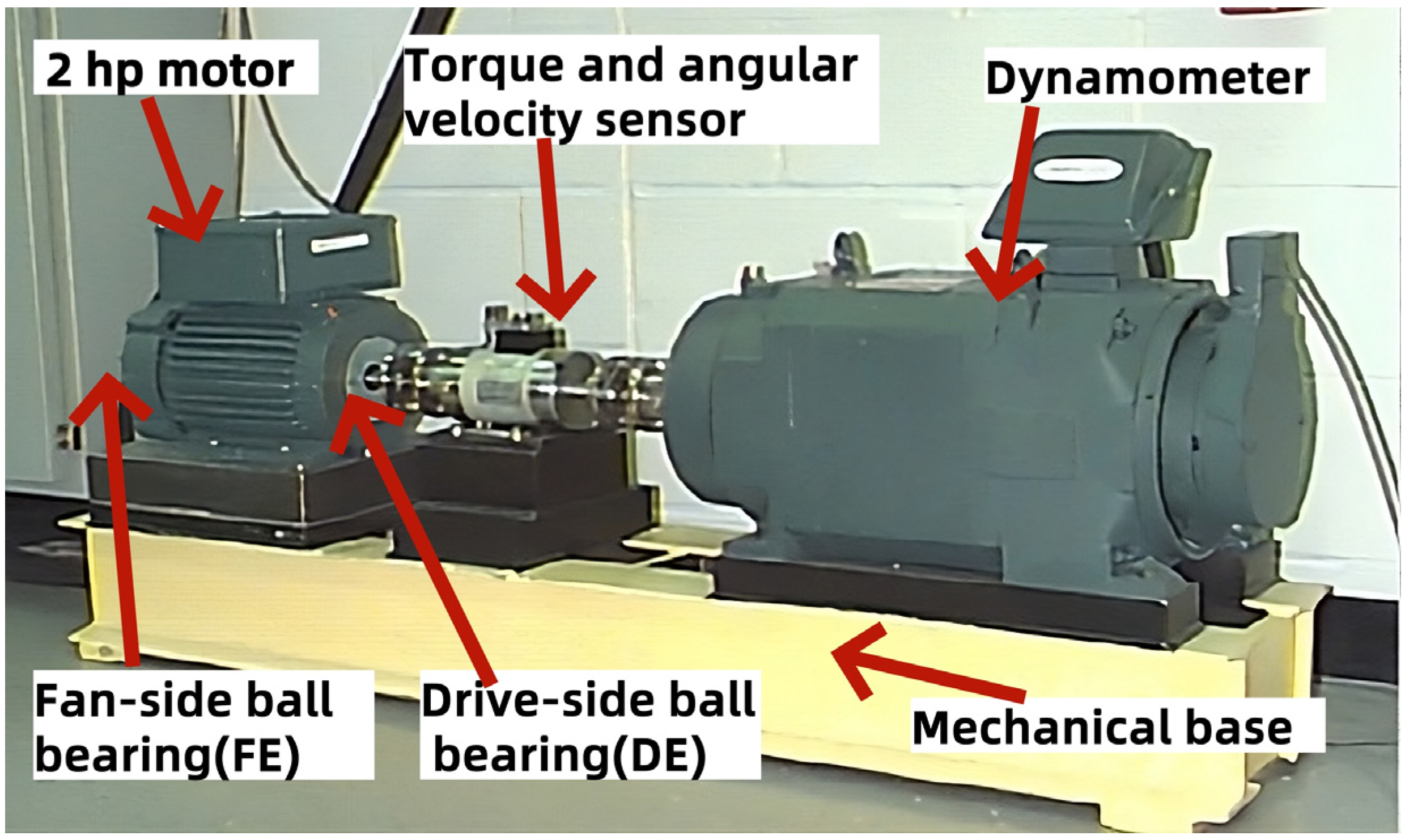
As shown in the Figure 1, the test bench was composed of a two-horsepower motor positioned on the left, a torque transducer with an integrated encoder located in the center, and a dynamometer placed on the right. Additionally, a control electronics system was employed to regulate the setup, though this is not shown in the illustration.

The data were collected for normal bearings, single-point drive-end faults, and fan-end faults. The sampling frequency was 12 kHz, except for the drive-end bearings, where it was 48 kHz. The number of samples ranged from 121,991 to 485,643. Motor bearings were intentionally damaged using electro-discharge machining (EDM), with faults introduced at various locations, including the inner raceway, rolling element (ball), and outer raceway. These faults varied in size, ranging from 0.007 inches to 0.040 inches in diameter. After introducing the faults, the bearings were reinstalled in the test motor, and vibration data were collected for motor loads ranging from 0 to 3 horsepower, corresponding to motor speeds between 1797 RPM and 1720 RPM.

There were 17 types of defects and one normal signal for the different loads (from 0 to 3 HP) related to each rolling defect. The defects for 1 HP load are listed as follows:

BALL _ 007 _ 1: Ball defect (0.007 inch)

BALL _ 014 _ 1: Ball defect (0.014 inch)

BALL _ 021 _ 1: Ball defect (0.021 inch)

BALL _ 028 _ 1: Ball defect (0.028 inch)

IR _ 007 _ 1: Inner raceway defect (0.007 inch)

IR _ 014 _ 1: Inner raceway defect (0.014 inch)

IR _ 021 _ 1: Inner raceway defect (0.021 inch)

IR _ 028 _ 1: Inner raceway defect (0.028 inch)

OR _ 007 _ 3 _ 1: outer raceway defect (0.007 inch, data collected from 3 o’clock position)

OR _ 014 _ 3 _ 1: outer raceway defect (0.014 inch, 3 o’clock position)

OR _ 021 _ 3 _ 1: outer raceway defect (0.021 inch, 3 o’clock position)

OR _ 007 _ 6 _ 1: outer raceway defect (0.007 inch, data collected from 6 o’clock position)

OR _ 014 _ 6 _ 1: outer raceway defect (0.014 inch, 6 o’clock position)

OR _ 021 _ 6 _ 1: outer raceway defect (0.021 inch, 6 o’clock position)

OR _ 007 _ 12 _ 1: outer raceway defect (0.007 inch, data collected from 12 o’clock position)

OR _ 014 _ 12 _ 1: Outer raceway defect (0.014 inch, 12 o’clock position)

OR _ 021 _ 12 _ 1: Outer raceway defect (0.021 inch, 12 o’clock position)

Normal 1: Normal

In this study, we used the complete CWRU data packet and all 17 types of defects. The data files were prepared in Matlab format and included vibration data from the fan end and drive end, as well as the motor’s rotational speed (RPM).

2.2. Teager–Kaiser

The Teager-Kaiser energy methods are techniques used in signal and image analysis [15]. They can reveal important structures and characteristics within signals through specific energy measurements. These methods involve calculating the energy of a modified signal, derived from the original signal through nonlinear operations. This modified energy provides valuable information of the signal’s amplitude, frequency, and other characteristics.

The general formula for calculating the Teager-Kaiser energy of a discrete signal x(n) is [16,17]:

$$E_{\mathrm{T}\mathrm{K}}\left(n\right)=x^2\left(n\right)-x(n-1)\cdot x(n+1)$$

(1)

where x(n) represents the value of the signal at time n, $E_{\mathrm{T}\mathrm{K}}\left(n\right)$ is the Teager-Kaiser energy at time n, and $x(n-1)\cdot x(n+1)$ refers to the product of the signal values shifted by one unit in time with respect to x(n).

In image analysis, these methods can be applied by treating an image’s pixels as signal samples and using similar operations to calculate the modified energy. However, it should be noted that while these methods are useful for extracting relevant features in certain signals and images, they are not suitable for all situations and may require adjustments depending on the specific application context.

The TKEO (Teager–Kaiser energy operator) was proposed by Kaiser and Teager as an approach to quantify the energy required for signal generation. It is primarily used to analyze rapid variations of energy in a signal. Unlike other methods based on power or amplitude measurements, the TKEO focuses on abrupt changes and the instantaneous evolution of the signal.

2.3. Support Vector Classifiers (SVCs)

Support vector classifiers (SVCs) are classification tools based on support vector machines (SVMs). The objective of an SVC is to identify the optimal hyperplane that effectively separates different classes of data, while maximizing the margin, which is defined as the distance between the hyperplane and the closest data points from each class. As showed in Figure 2, in 2D, the hyperplane is a line who divides the plane into two halves(red and green); in 3D, it is a plane who splits 3D space into two regions. However, not all data points impact the placement of this boundary. Only the points nearest to the hyperplane, known as support vectors, influence its position and orientation. These critical points define the margin, effectively ‘supporting’ the optimal boundary. Maximizing the margin based on these support vectors enhances the classifier’s ability to generalize effectively to new data.

To determine the optimal hyperplane using an SVC, the problem is formulated as a convex optimization problem [19]. Constraints are applied to ensure that data points are at least one unit distance from the hyperplane, creating a wide-margin separation. In real-world applications, however, data are often not perfectly separable. The SVC addresses this through a soft margin approach, introducing a tolerance parameter C that allows some points to be misclassified. This enables the model to maximize the margin while tolerating a certain level of error. The value of C controls tolerance in relation to misclassification: higher C reduces tolerance of error, seeking a stricter separation, while a lower C allows more flexibility.

The optimization objective of an SVC can be expressed as follows [20]:

$$\underset{\mathbf{w},b}{\min }{\displaystyle \frac{1}{2}}{‖\mathit{w}‖}^2+C\sum _{\mathcal{i}=1}^{\mathrm{n}}{\xi }_{\mathcal{i}}$$

(2)

where w is the weight vector of the hyperplane, ‖w‖² represents the squared norm, which is minimized to maximize the margin between classes, and b is the bias term, which adjusts the position of the hyperplane. ${\xi }_{\mathcal{i}}$ are the slack variables that allow certain data points to violate the margin constraints, and C balances the trade-off between maximizing the margin and tolerating misclassifications, as reflected in the optimization objective.

The classification constraints for each data point are given as follows:

$${\mathcal{y}}_{\mathcal{i}}\left(\mathit{w}·{\mathit{x}}_{\mathcal{i}}+b\right)\ge 1-{\xi }_{\mathcal{i}}, \forall \mathcal{i}=1,2,\dots ,\mathrm{n}$$

(3)

where ${\mathcal{y}}_{\mathcal{i}}$ represents the label of the i-th data point (+1 or −1), ${\mathit{x}}_{\mathcal{i}}$ is the feature vector of the i-th data point, and the notation $\forall \mathcal{i}$ = 1, 2, …, n, indicates that the constraint applies to all n data points.

This constraint ensures that correctly classified points are on the correct side of the hyperplane and have a margin of at least 1. For points within the margin or misclassified, ${\xi }_{\mathcal{i}}$ ≥ 0 accounts for the violation.

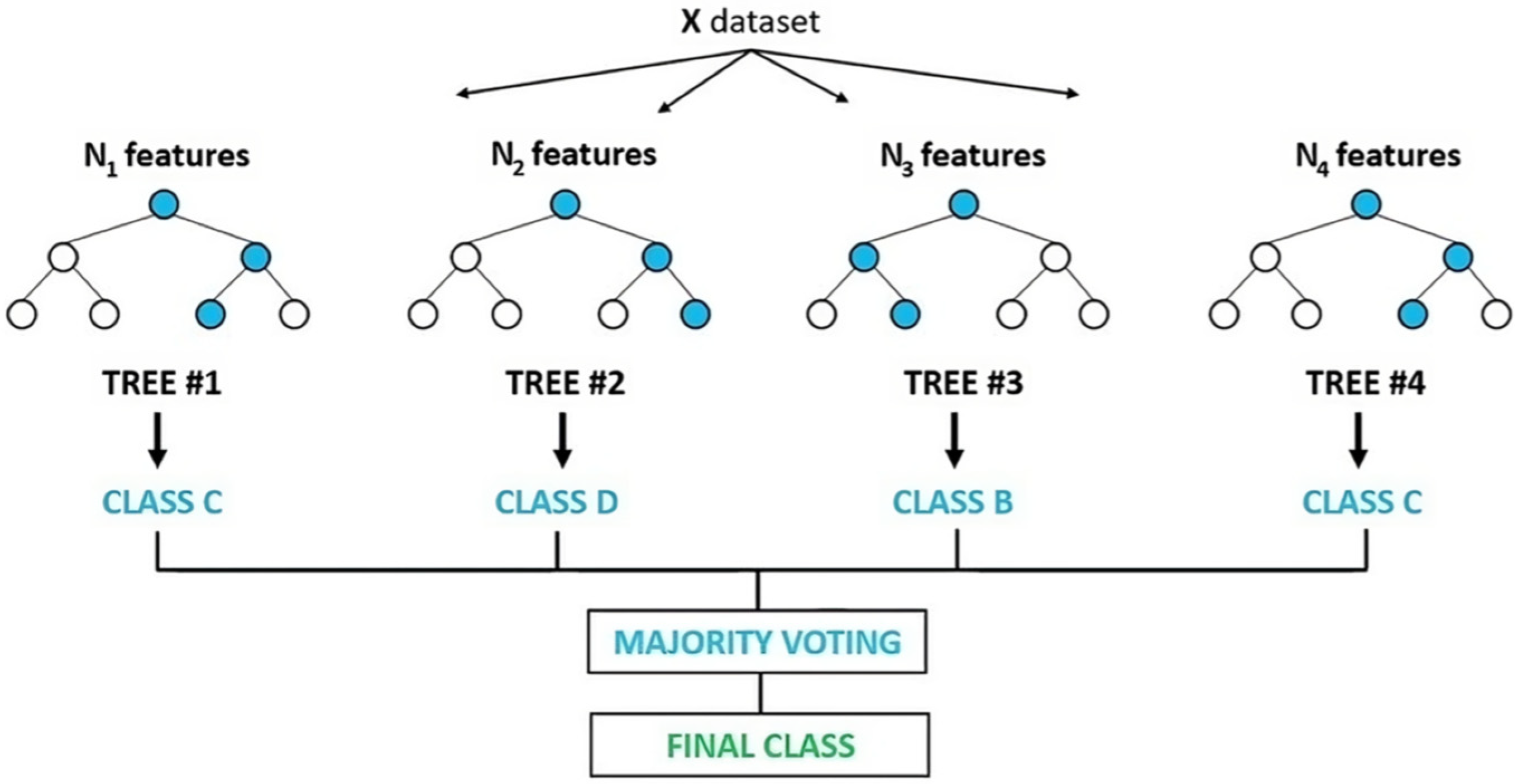
2.4. Random Forest Classifier (RFC)

Random forest is widely used as a supervised learning algorithm in both classification and regression tasks [21]. It uses the idea of ensemble learning, where multiple decision trees are trained on different subsets of the dataset to improve model performance.

The name ‘random forest’ reflects its operation as a classifier that encompasses multiple decision trees, each trained on different subsets of the given dataset. The goal is to enhance the model’s overall predictive accuracy. Rather than depending on a single decision tree, random forest combines the predictions of multiple trees, with the final output determined by majority voting for classification or averaging for regression.

Classification Process in Random Forest, as illustrated in Figure 3 [22]:

• Construction of Decision Trees: Random forest generates multiple decision trees, each trained on a random subset of the training data and features. As shown in the image, Tree #1, Tree #2, Tree #3, and Tree #4 are constructed using different subsets of features (N_features), ensuring diversity in the model.
• Individual Predictions: Each decision tree independently predicts the class of the input data. In the image, Tree #1 predicts Class C, Tree #2 predicts Class D, Tree #3 predicts Class B, and Tree #4 predicts Class C.
• Majority Voting: The predictions from all trees are aggregated, and the final class is determined by majority vote. In the illustration in the image, the majority voting process results in a final prediction of Class C.

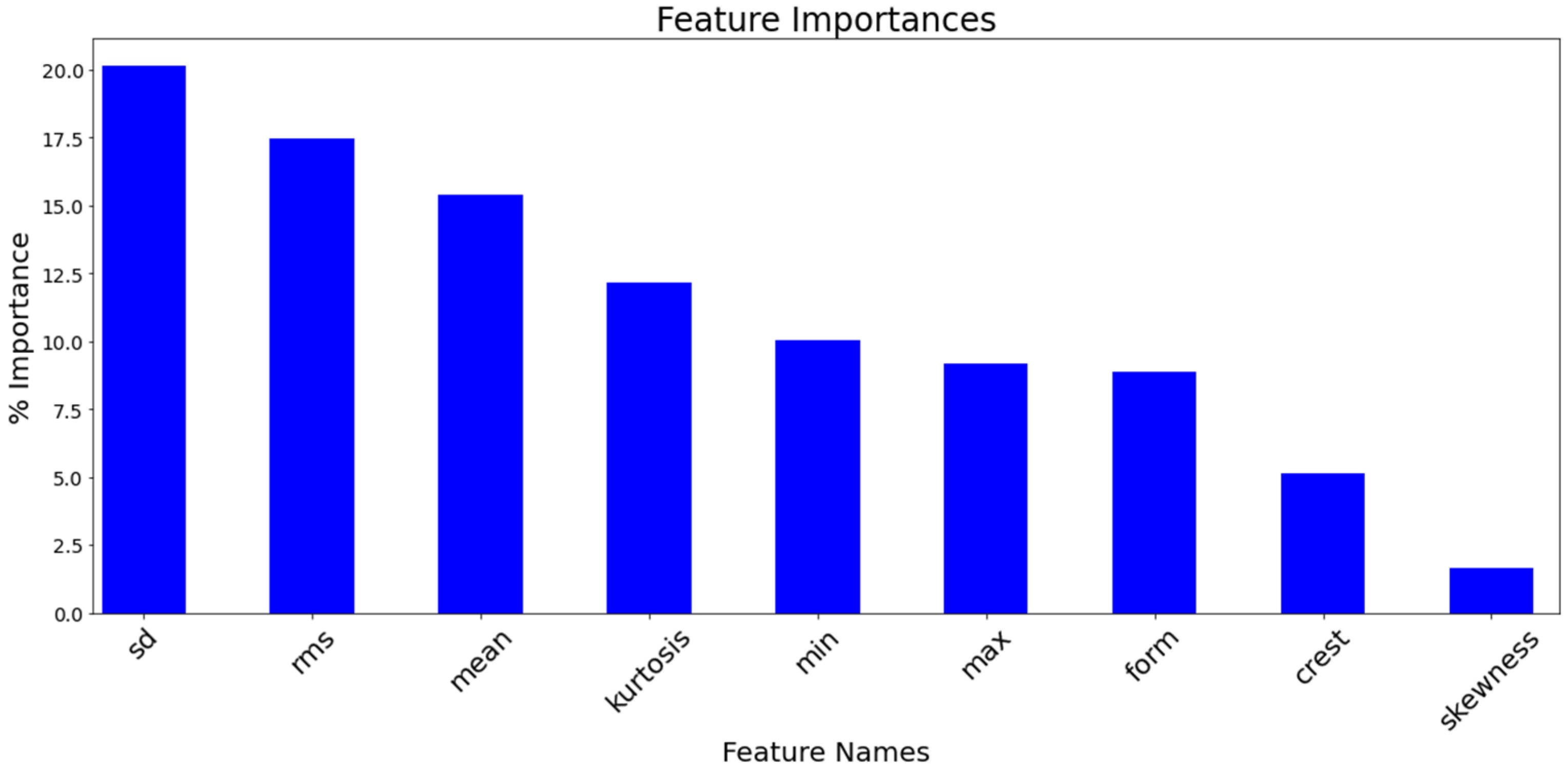
2.5. Features Used

After reviewing the literature on Teager–Kaiser energy methods and applying programs on Kaggle such as SVC [24] and RFC [25], we identified the following 9 features used in these two models:

• Max: x_max, the maximum value;
• Min: x_min, the minimum value;
• Mean: μ = (Σx)/N;
• SD (standard deviation): σ = √[(Σ(x − μ)²)/N], the square root of the sum of squares of deviations from the mean, divided by the total number of values;
• RMS (root mean square): √[(Σx²)/N];
• Skewness: (Σ(x − μ)³)/[N · σ³], the skewness of distribution relative to the mean indicates whether values lean more to the left or right;
• Kurtosis: (Σ(x − μ)⁴)/[N · σ⁴] − 3. Kurtosis measures the shape of the distribution. Positive kurtosis indicates values that are more concentrated around the mean (more peaks and troughs), while negative kurtosis indicates a flatter distribution compared with the normal pattern;
• Crest: x_max/x_eff, the ratio of the highest peak of the wave to its effective value.
• Form: The shape of a signal that can describe its structure, frequency content, or other specific characteristics.

The Figure 4 illustrates the importance of various features in the model. The last three features—form, crest, and skewness—each have an importance of less than 10%, as shown by the lower bars. This low importance is likely to be because these features provide limited additional information beyond what has already been captured by the six key features (e.g., RMS, Standard Deviation, and Kurtosis). For example, standard deviation is indirectly reflected in the calculations of skewness and crest, reducing their independent contribution. By removing these less important features, the model becomes simpler, more computationally efficient, and less prone to overfitting, while maintaining high predictive accuracy.

2.6. Data Segment Length

In the diagnosis of vibration faults, determining the appropriate length of signal segments is crucial. Evaluation involving different segment lengths revealed that these significantly influenced the model performance. To effectively capture vibration signal features across different sampling rates, this study categorized the acquired signals into two lengths: 2400 and 12,000 data points.

A 2400-point segment represents approximately 5–6 rotational cycles at a 12 kHz sampling rate and about 1.5 cycles at 48 kHz. In comparison, a 12,000-point segment corresponds to approximately 29 cycles at 12 kHz and 7 cycles at 48 kHz. This dual-segment strategy ensured the extraction of vibration features over both short and extended time durations.

The 2400-point segment focused on capturing high-frequency variations within a shorter duration, making it suitable for real-time monitoring and detection of high-frequency fault features. This is particularly advantageous at the higher sampling rate (48 kHz), where computational efficiency is a critical factor. Conversely, the 12,000-point segment spanned more rotational cycles, allowing the effective analysis of low-frequency periodic variations in the frequency domain, making it ideal for identifying deeper fault patterns.

By adopting this dual-segment strategy, the current study achieved a balance between high-resolution time-domain features and comprehensive frequency-domain analysis, leveraging the strengths of both short- and long-duration signal segments.

2.7. Computational Complexity

In the fields of machine learning and data analysis, the computational complexity of algorithms is a critical consideration, especially when dealing with large-scale datasets or real-time applications. Understanding the complexity of an algorithm not only helps evaluate its computational efficiency but also provides a theoretical foundation for optimizing model performance. Support vector machines and random forests have complexities that depend on factors such as the number of features, the number of samples, and the model structure. This section discusses the computational complexity of these two algorithms and analyzes how reducing the number of features can optimize the computational efficiency of the model.

2.7.1. SVM Complexity

The time complexity of an SVM with a nonlinear kernel is generally as follows:

$$O(n^2\times d)$$

(4)

where n is the number of samples, d is the number of features, and the term $n^2$ arises from the computation of the Gram matrix (dot products between all points in the feature space).

For a linear SVM, the optimization complexity is O(n × d), which is faster.

2.7.2. RF Complexity

The computational complexity of a random forest depends on several factors, as follows:

-

Training phase:

$$\begin{gathered} \mathrm{s}\mathrm{i}\mathrm{n}\mathrm{g}\mathrm{l}\mathrm{e} \mathrm{d}\mathrm{e}\mathrm{c}\mathrm{i}\mathrm{s}\mathrm{i}\mathrm{o}\mathrm{n} \mathrm{t}\mathrm{r}\mathrm{e}\mathrm{e}:O(n\times d\times h) \\ \mathrm{r}\mathrm{a}\mathrm{n}\mathrm{d}\mathrm{o}\mathrm{m} \mathrm{f}\mathrm{o}\mathrm{r}\mathrm{e}\mathrm{s}\mathrm{t} \mathrm{w}\mathrm{i}\mathrm{t}\mathrm{h} \mathrm{T} \mathrm{t}\mathrm{r}\mathrm{e}\mathrm{e}\mathrm{s}:O(T\times n\times d\times h) \end{gathered}$$

(5)

-

Prediction phase:

$$\begin{gathered} \mathrm{s}\mathrm{i}\mathrm{n}\mathrm{g}\mathrm{l}\mathrm{e} \mathrm{d}\mathrm{e}\mathrm{c}\mathrm{i}\mathrm{s}\mathrm{i}\mathrm{o}\mathrm{n} \mathrm{t}\mathrm{r}\mathrm{e}\mathrm{e}:O\left(h\right) \\ \mathrm{r}\mathrm{a}\mathrm{n}\mathrm{d}\mathrm{o}\mathrm{m} \mathrm{f}\mathrm{o}\mathrm{r}\mathrm{e}\mathrm{s}\mathrm{t} \mathrm{w}\mathrm{i}\mathrm{t}\mathrm{h} \mathrm{T} \mathrm{t}\mathrm{r}\mathrm{e}\mathrm{e}\mathrm{s}:O(T\times h) \end{gathered}$$

(6)

where n is the number of data samples, d is the number of features, h is the average depth of the trees, and T is the number of trees in the forest.

Therefore, all other things being equal, when the features are fewer in number, the computational complexity is lower. In practice, it may be useful to select the most relevant features to avoid unnecessarily increasing the complexity.

3. Experimental Procedure

This study employed vibration signal data from the CWRU dataset to perform fault diagnosis in rotating machinery, using a random forest classifier and a support vector classifier. The detailed experimental procedure is outlined as follows.

3.1. Data Processing and Feature Extraction

For each load condition, the vibration signals were segmented into two types according to the data length: 2400-point segments and 12,000-point segments. These segments were subjected to two processing approaches, as follows:

• Raw Signal Processing: Features were directly extracted from the raw vibration signals;
• TKEO Processing: The Teager–Kaiser energy operator was applied to highlight transient energy changes in the signal, enhancing fault-related features.

From each segment, two feature sets were extracted, as follows:

• Six-Parameter Set: This set included Max, Min, Mean, Standard Deviation, RMS, and Kurtosis;
• Four-Parameter Set: This reduced feature set comprised Mean, Standard Deviation, RMS, and Kurtosis, aiming to evaluate model performance within a lower-dimensional feature space.

3.2. Data Splitting and Standardization

The data were divided into training and testing sets in an 80/20 ratio, ensuring stratification according to fault categories. Stratified sampling ensured that the distribution of target labels remained consistent between the training and testing datasets, mitigating potential biases caused by class imbalance.

To eliminate the influence of feature magnitudes, all data were standardized using the StandardScaler method. Standardization transformed the features to zero mean and unit variance.

3.3. Model Training and Optimization

• Random Forest Classifier:

The RFC model was configured with 300 decision trees and employed the ‘square root rule’ for feature selection at each split. This setup balanced generalization performance and computational efficiency. The model was trained using parallel processing to maximize resource utilization.

• Support Vector Classifier:

An initial SVC model was trained with default parameters. To enhance performance, hyperparameter optimization was performed using GridSearchCV 1.3.0. The grid search focused on tuning the following parameters:

• C: regularization parameter (values: 1, 10, 45, 47, 49, 50, 51, 55, 100, 300, 500);
• Gamma: kernel coefficient (values: 0.01, 0.05, 0.1, 0.5, 1, 5);
• Kernel: radial basis function kernel (‘rbf’).

A 10-fold cross-validation strategy was employed to ensure robust performance across different data splits. The best parameter combination was used to train the final model, which was evaluated on the test dataset.

3.4. Performance Evaluation

The models’ performance was evaluated using the following metrics:

• Accuracy: The percentage of correctly classified samples out of the total samples, serving as a primary indicator of overall performance;
• Confusion Matrix: a detailed breakdown of classification outcomes for each fault category, including true positives, true negatives, false positives, and false negatives for each fault category.
• Classification Report: a summary of metrics such as precision, recall, and F1 score, offering a comprehensive view of the models’ strengths and weaknesses in fault classification.

4. Results

The results were obtained on a Windows system using Ubuntu 20.04 LTS within the Windows Subsystem for Linux (WSL). To manage the environment, we used Anaconda 23.7.2, running Python 3.11.4 for model training. The setup included an Intel i5-13500HX processor and an NVIDIA GeForce RTX 4060 GPU, whose powerful computational capabilities reduced the training time to under five seconds.

The following results represent the highest accuracies obtained:

• 1HP: 745.7W (Motor power).
• 2400 et 12,000: Number of samples per segment for training.
• 2400teo et 12,000teo: Data processed with the Teager–Kaiser energy method.
• SVC6 et RFC6: Results based on six features: Mean, Standard Deviation, RMS, Kurtosis, Max, Min.
• SVC4 et RFC4: Results based on four features: Mean, Standard Deviation, RMS, Kurtosis.

Based on the results presented in

Table 1. Results: Accuracy Percentage.

Load	Data Type	Support Vector Classifier		Random Forest Classifier
Load	Type	SVC6	SVC4	RFC6	RFC4
0HP	2400	99.07%	99.07%	98.25%	98.25%
	2400teo	93.93%	91.59%	97.08%	92.98%
	12,000	97.67%	97.67%	97.06%	100.00%
	12,000teo	95.35%	95.35%	94.12%	91.18%
1HP	2400	97.91%	97.49%	97.91%	97.91%
	2400teo	94.98%	94.14%	97.38%	95.29%
	12,000	95.83%	95.83%	100.00%	100.00%
	12,000teo	91.67%	81.25%	100.00%	94.74%
2HP	2400	99.65%	98.96%	99.57%	98.27%
	2400teo	97.23%	95.50%	99.13%	99.13%
	12,000	98.28%	98.28%	97.83%	97.83%
	12,000teo	94.83%	93.10%	100.00%	100.00%
3HP	2400	99.16%	97.91%	100.00%	99.48%
	2400teo	94.98%	93.72%	98.95%	97.91%
	12,000	100.00%	100.00%	100.00%	97.37%
	12,000teo	93.75%	91.67%	100.00%	100.00%

, we conducted data analysis to derive

Table 2. Average Accuracy for Loads from 0 to 3HP.

Type	SVC6	SVC4	RFC6	RFC4
2400	98.95%	98.36%	98.93%	98.47%
2400teo	95.28%	93.74%	98.14%	96.33%
12,000	97.95%	97.95%	98.72%	98.80%
12,000teo	93.90%	90.34%	98.53%	96.48%

and

Table 3. Average Accuracy for Loads from 1 to 3HP.

Type	SVC6	SVC4	RFC6	RFC4
2400	98.91%	98.12%	99.16%	98.55%
2400teo	95.73%	94.45%	98.49%	97.44%
12,000	98.04%	98.04%	99.28%	98.40%
12,000teo	93.42%	88.67%	100.00%	98.25%

.

Table 2 and Table 3 lead us to the following conclusions: While the TKEO method generally showed slightly lower performance compared with traditional approaches, it demonstrated outstanding accuracy under specific conditions, such as with RFC6, 12,000 samples, and a high load (HP > 0). This highlights TKEO’s potential effectiveness in scenarios involving higher mechanical loads.

On the other hand, for low loads (0HP), SVC outperformed RFC. Interestingly, with 0 HP and a smaller dataset (2400 samples), SVC achieved better accuracy than with the larger dataset (12,000 samples). Considering the number of variables, the difference between using four and six variables was generally small for the traditional methods, often within 0.6%. However, for small datasets or when using TKEO, the four-variable configuration occasionally outperformed the six-variable setup. This observation suggests that the choice of variables and dataset size has a nuanced impact on model performance, depending on the method used.

As detailed in

Table 4. Evaluation of SVC and RFC Models with Six and Four Features.

	SVC6	SVC4	RFC6	RFC4
Mean	96.52%	95.10%	98.58%	97.52%
SD	0.024	0.045	0.016	0.026
RMS	0.965	0.951	0.985	0.975
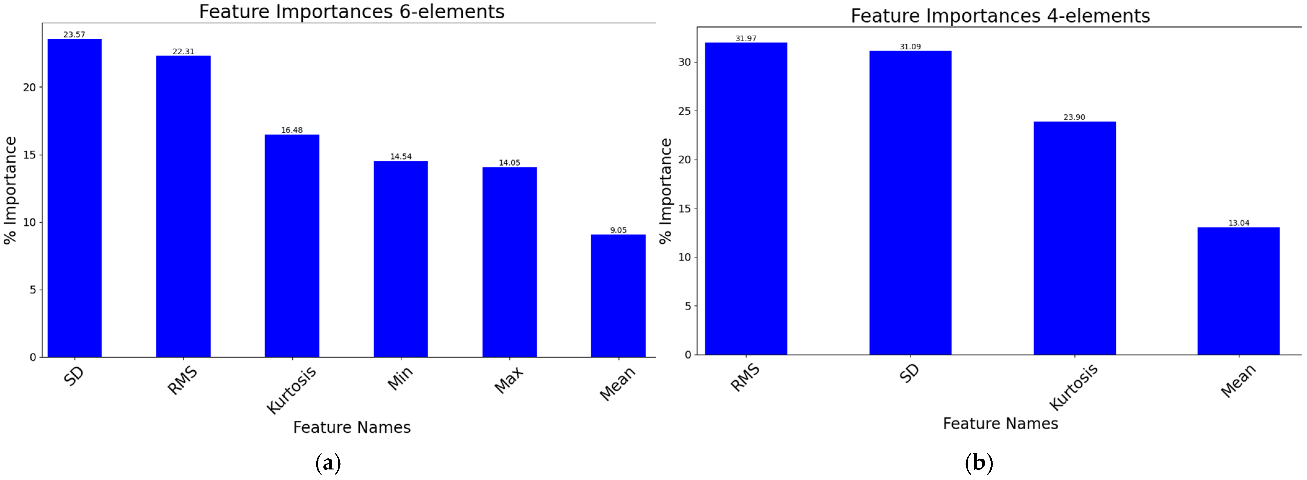
Kurtosis	−0.838	5.328	2.210	0.873

comparing SVC and RFC models with six versus four features, the RFC models, RFC6 and RFC4, both demonstrated high average accuracy, with RFC6 achieving 98.58%. This indicates that the random forest classifier outperformed the support vector classifier on this dataset. Additionally, the RFC models exhibited lower standard deviation; particularly, RFC6 had a standard deviation of just 0.016. This low variability suggests that RFC6 can provide more stable performance across multiple experiments or data splits. Observing the RMS and kurtosis metrics, RFC6 also showed the highest RMS (0.985), indicating that its accuracy distribution was closer to the ideal level.

When using only four features (mean, standard deviation, RMS, and kurtosis), both SVC and RFC models maintained relatively high accuracy, though this was slightly lower than their six-feature counterparts. Notably, RFC4 achieved an accuracy of 97.52%. In fact, the minimum and maximum calculations required almost no additional resources. The cost of calculation was not relevant. Rather, it was sufficient to keep only the four parameters. These sufficiently characterized a normal distribution, an assumption that was easily verified; consequently, these parameters were deemed sufficiently contributive, as seen in the example (see Figure 5).

To illustrate the model’s capability, we analyzed the ‘SVC6 2400, 2HP, 99.65% accuracy’ case in detail. This example was selected due to its exceptional performance in the high-load scenario (2HP), fault detection in this kind of scenario may be critical for preventing catastrophic failures. The subsequent feature importance analysis (Figure 5a) and the confusion matrix (Figure 6 and Figure 7) further demonstrated how the TKEO-enhanced features enabled precise discrimination of faults, even under complex vibration patterns. This case exemplifies the framework’s balance between accuracy and computational efficiency, a key requirement for real-time industrial deployment.

Based on these figures, the following can be stated regarding SVC6 (2400, 2HP, 99.65% accuracy) and SVC4 (2400, 2HP, 98.96% accuracy):

• SD, RMS, and kurtosis are the most important features, with a critical role in capturing vibration signal variations and fault patterns;
• Focusing on RMS, SD, and kurtosis as primary features, with mean as a complementary feature, can further enhance model performance;
• Reducing the number of features (from 6 to 4) simplified the model but did not significantly affect its core performance, as RMS and SD remained the key contributors;
• For higher accuracy, the use of more features (Min and Max) could provide additional diagnostic insights regarding specific fault types.

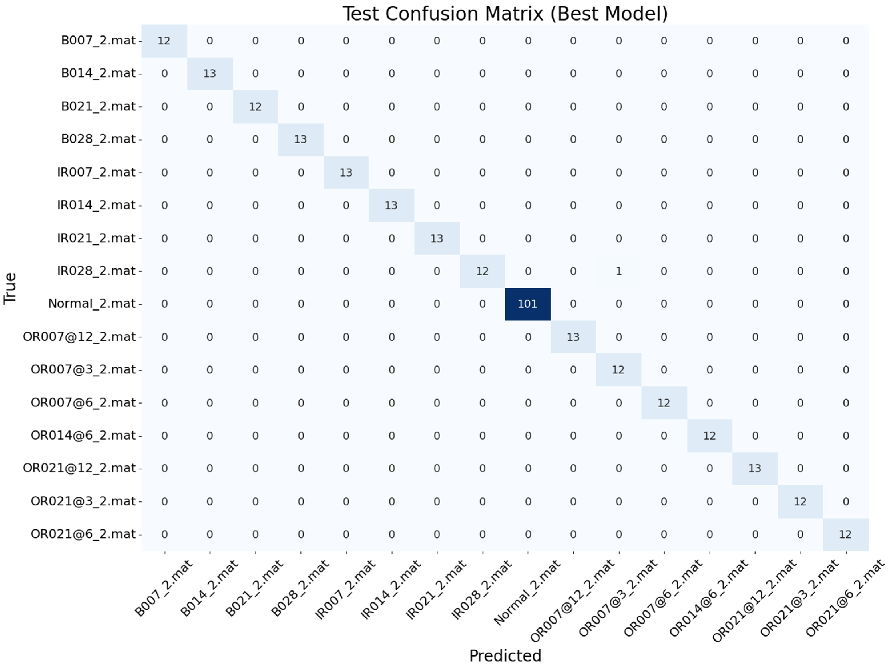
The confusion matrices for both the training and testing phases (Figure 6 and Figure 7) provide a comprehensive visualization of the model’s classification performance. Each row in the matrix represents the actual class, while each column represents the predicted class. The diagonal elements indicate the number of correctly classified samples, while the off-diagonal elements highlight misclassifications.

For example, in Figure 6 (training phase), the diagonal value of 36 for the actual class ‘OR007@12_2.mat’ indicates that 36 samples were correctly classified. However, the off-diagonal value of 1 in the predicted class ‘OR021@12_2.mat’ suggests that one sample was misclassified.

The confusion matrix offers another view of the model’s performance, allowing us to draw the following conclusions:

• The model correctly classified the ‘Normal_2.mat’ class in the majority of instances across both the training and testing phases, indicating its ability to reliably distinguish normal data from fault classes;
• Misclassifications were observed between the ‘OR007@12_2.mat’ and ‘OR021@3_2.mat’ classes, as well as between ‘OR007@6_2.mat’ and ‘OR014@6_2.mat’ during training. These results indicate that these fault types share similar features, sometimes leading to confusion during training;
• The primary misclassification observed in the testing phase occurred between the ‘IR028_2.mat’ and ‘OR007@3_2.mat’ classes. This suggests that although the model performed exceptionally well overall, certain types of fault exhibited overlapping characteristics that made them more difficult to distinguish in testing.

The high classification accuracies reported in this section (e.g., 99.65% for SVC6 at 2HP) directly reflect the model’s capability to distinguish different types of critical fault (e.g., inner race defects vs. ball defects) in real-world diagnostic scenarios.

• Practical Implications: 99.65% accuracy implies that only 3 out of every 1000 fault detections would result in misclassification, which should significantly reduce unplanned downtime. For instance, in wind turbine applications, this level of reliability could prevent catastrophic failures and save up to USD 120,000 annually in maintenance costs (He et al., 2023) [26].
• Links to Diagnostics: As highlighted by experimental studies, excellent classification results in the testing phase enable the accurate categorization of fault signals into the correct types. This capability is fundamental to diagnostics, as it enables for the timely and precise identification of bearings’ states of health, which is critical for predictive maintenance. The confusion matrices (Figure 6 and Figure 7) further validate the model’s diagnostic precision, showing minimal misclassification between fault categories.

These results reveal that the framework not only achieved high classification accuracy but that it can also provide actionable insights into the health of bearings, enabling proactive maintenance decisions.

5. Discussion

5.1. Ease of Implementation

In this study, the data preprocessing steps included data normalization (centering and standardization) and splitting the data into training and testing sets. The CWRU bearing signals were relatively clean; so, they could be processed without additional noise filtering. However, to further test the model’s robustness, we introduced white noise and applied singular spectrum analysis (SSA) [27], which effectively extracted significant components from the time series, revealing the underlying structure and patterns in the signal.

For hyperparameter tuning, we used GridSearchCV1.3.0, which exhaustively searched through all possible combinations of parameters to find the optimal model configuration. To speed up this process, RandomizedSearchCV was employed; parameter combinations were randomly sampled to find an approximate optimal range, thus reducing computation time.

All experiments were conducted using the scikit-learn library, which provided comprehensive and mature support for the machine learning algorithms, making the implementation of the experiments more straightforward.

SVCs require strict normalization of the data, and the selection of hyperparameters is relatively complex. In contrast, RFCs do not have strict requirements regarding data distribution and they also possess built-in processing capabilities, making them easier to implement. Additionally, RFCs have fewer hyperparameters, which makes them suitable for quick implementation.

5.2. Robustness

In terms of noise and missing values, the RFC demonstrated greater robustness. By integrating multiple decision trees, the RFC was able to tolerate more noise and interference. On the other hand, the SVC, while capable of finding the optimal hyperplane in high-dimensional feature space, showed weaker robustness in the presence of noise.

The experimental results showed that, under different RPM and charge conditions, the classification accuracy of the SVC significantly decreased, from 98.9% to 85.3%, as the noise levels increased. In contrast, the RFC maintained higher accuracy under the same conditions, dropping from 99.2% to 94.8%, indicating its stronger tolerance of noise.

5.3. Computational Complexity Comparison

By segmenting the data and using the Teager–Kaiser energy method, the model training time was significantly optimized. For example, using the same data, when segmented into 2400 data points, the six features processed using traditional methods resulted in a data size of 854 × 6. When segmented into 12,000 data points, the six features processed using traditional methods resulted in a data size of 171 × 6. With an older GPU, training time typically remained under 1 min; using a newer graphics card, training time can be reduced to just a few seconds.

However, the computational complexity comparison of different methods cannot be quantified by a single indicator. Although time complexity, space complexity, the number of parameters, running time, memory usage, and other dimensions can be considered separately, it is difficult to use a unified quantitative standard to directly compare methods, due to differences in algorithmic structure, preprocessing requirements, hardware dependence, etc. This situation requires combining specific experimental design and application scenarios and comprehensively evaluating indicators from multiple angles to obtain a more reasonable comparison.

However, it is still possible to discuss comparison of computational complexity under similar conditions. For example, if we go from 4 to 6 or 11 features, the impact on complexity depends on the type of SVC; with a nonlinear kernel (RBF), computational complexity increases from $O(n^2\times 4)$ to $O(n^2\times 6)$ or $O(n^2\times 11)$, where n is the number of samples.

Therefore, all else being equal, with 6 or 11 features, the algorithm takes about 1.5 or 2.75 times longer than with 4 features. If the number of samples is large, the impact of going from 4 to 11 features can become significant, especially for SVMs with nonlinear kernels.

RFC training time increased linearly with the amount of data, especially when the dataset exceeded 50,000 records, at which point the training time increased significantly. In contrast, SVCs are faster to train on smaller datasets, but as the data size and feature count grew, the computational complexity increased substantially.

5.4. Summary and Recommendations

To contextualize our contributions,

Table 5. Comparison of the present study implications with the reported literature using CWRU datasets.

Authors	Datasets	Feature Extraction	Features	Classifier	Accuracy	Classes of Problem
Yoo et al. (2023) [6]	CWRU	Downsample signals and generate spectrogram using STFT	Spectrogram	Lite CNN	99.92%	10 classes
Souaidia and Thelaidjia (2024) [7]	CWRU	Statistical features (time domain)	9 statistical features	LR, RF, SVM	LR: 99.02% RF: 98.00% SVM: 99.22%	10 classes
Alonso-González et al. (2023) [8]	CWRU	Extract amplitude information (envelope and frequency-domain analysis)	BPFI/BPFO amplitude (5 features)	KNB, DT (Fine Tree), Fine KNN	KNB: 94.4% DT & KNN: 100%	3 classes
Hadi et al. (2023) [28]	CWRU	Normalization, data balancing, and categorical encoding	9 time-domain/frequency-domain features	RF (PyCaret) and AutoDNN (AutoKeras)	Training 99.70% (PyCaret), Test 97.00% (AutoKeras)	10 classes
Shi et al. (2022) [29]	CWRU, Xi’an Jiaotong University Bearing Life Data	Improved TKEO method; combined bandpass filtering and weighted summation to suppress Gaussian white noise	Components selected based on Pearson correlation coefficient	Not specified (focus on improved TKEO signal processing)	Clear fault frequency identification and faster computation than traditional TKEO/EEMD-SK/PSO-VMD	2 classes (early fault/normal)
Dhaval V. Patel et al. (2023) [11]	CWRU, IMS, PU, MFPT	TKEO + SSA TKEO enhanced pulse signature; extracting fault frequency through SSA (L = N/2, r = 2)	Frequency analysis	No traditional classifier (frequency analysis)	CWRU: 95–100% for inner/outer race fault	4 classes (normal/IR/O R/rolling element faults)
Shilpi Yadav et al. (2023) [12]	CWRU, IIT Kanpur	Extracted 11 statistical features from original, Hilbert-transformed, and TKEO signals	11 statistical features	LR, LDA, KNN, CART, NB, SVM	CWRU: All models with TKEO features achieved 100%	2 classes (normal/rolling element faults)
Saufi et al. (2021) [13]	CWRU	TKEO preprocessing, conversion to 28 × 28 image blocks	784 image features; 9 statistical features	DSAE, ANN	DSAE + ALO: 99.5%; ANN (statistical features): 89%; ANN (image features): 77.2%	4 classes (normal, OR, IR, rolling element faults)
Xuanbai YU, Olivier CASPARY	CWRU	TKEO preprocessing (enhancing transient energy changes) Extract 6 statistical features, optimized to 4 by removing low-contribution features (Max and Min)	4–6 statistical features	SVC, RFC	SVC6: up to 100% (12k samples, 3HP); RFC6: 98.58%; SVC4: 95.10%; RFC4: 97.52%; Under high load and large sample size: RFC4 reached 100% at 12k samples	18 classes (normal and 17 defects)

synthesizes critical methodological choices and performance outcomes from recent studies on bearing fault diagnosis. The comparison focuses on four dimensions: (1) feature extraction strategies, (2) classifier architectures, (3) dataset utilization, and (4) accuracy-class complexity tradeoffs.

In summary, under the experimental conditions of the current study, the random forest classifier provided a good balance between ease of implementation, robustness, and computational complexity; particularly, it demonstrated stability in the presence of noise. However, the computational complexity of the RFC increased linearly with the size of the dataset, suggesting that more computational resources may be needed for large-scale datasets.

On the other hand, support vector classifiers offer better classification performance on smaller datasets, especially when the data distribution is more complex. An SVC is capable of finding the optimal hyperplane in high-dimensional feature space. However, SVMs require more stringent data preprocessing and hyperparameter tuning, and their computational complexity significantly increases with the growth of the dataset.

Ultimately, the choice of algorithm should be based on the specific application scenario and experimental requirements. If the focus is on tasks involving noisy environments with lower computational resource demands, RFC is a better choice. If the dataset is smaller and higher classification accuracy is required, an SVC may perform better.

While the TKEO method may show slightly lower performance compared with traditional approaches in general, its computational efficiency makes it particularly advantageous when working with large datasets. This is because TKEO requires fewer calculations, making it more suitable for scenarios where processing time and computational resources are critical. Moreover, under specific conditions, such as high mechanical load (HP > 0) or larger datasets (e.g., 12,000 samples), TKEO demonstrated strong accuracy, showing its potential to be highly effective in those settings.

5.5. Future Applications and Practical Solutions

The proposed framework integrates the Teager–Kaiser Energy Operator (TKEO) method with machine learning algorithms (e.g., random forest and support vector machine), demonstrating significant advantages in practical applications. Compared with existing AI-based methods, our approach offers stronger potential and broader applicability, particularly in terms of robustness against noise, low data dependency, computational efficiency, and rapid deployment. These advantages make it highly suitable for real-time monitoring and fault diagnosis in complex industrial environments.

Based on these advantages, the proposed method has broad application prospects, especially in the following fields:

• Real-Time Vibration Monitoring and Fault Diagnosis in Industrial Equipment

In noisy industrial environments, real-time monitoring and fault diagnosis are critical for ensuring the safety and efficiency of production. By leveraging TKEO to extract key vibration features, our method achieved stable performance even with limited data and high noise levels. Compared with deep learning approaches (e.g., CNN and LSTM), our framework offers lower computational complexity and faster training speeds, making it highly suitable for real-time industrial diagnostics.

2.

Fault Detection in Wind Turbines

Wind turbines often operate in environments where obtaining large amounts of labeled data is challenging. Our method effectively extracts useful features from small datasets and employs RFC and SVC for efficient fault detection. Unlike deep learning methods (e.g., CNN and LSTM), which require extensive training data and longer training times, our approach reduces data dependency while maintaining high accuracy, making it more practical for real-world applications.

3.

Fault Diagnosis in Smart Home Appliances

Smart home appliances (e.g., air conditioners, refrigerators) require fast and cost-effective fault diagnosis solutions. Our method can operate efficiently on low-resource devices, providing rapid fault identification and diagnosis. Compared with deep learning methods (e.g., DNN), our approach is simpler to implement and has lower computational overhead, enabling quicker responses to appliance failures.

4.

Health Management in Smart Grids

Fault detection in critical grid components (e.g., transformers, switchgear) is essential for maintaining the reliability of power systems. By monitoring vibration signals in real time, our method can identify potential faults and issue early warnings. Compared with traditional methods (e.g., XGBoost), our approach demonstrated superior robustness to noise and faster training speeds, meeting the high demands of real-time performance and cost-effectiveness in power grids.

5.

Health Monitoring of Aircraft Engines

Fault detection in aircraft engines requires high accuracy, real-time performance, and the ability to train effectively with limited labeled data. Through optimized feature selection and data processing strategies, our method achieved high robustness and accuracy with rapid training on small datasets. Compared with deep neural networks, our approach not only reduces data requirements but also provides real-time diagnostics for resource-constrained systems.

In addition, the proposed method exhibits strong generalizability and can be applied to the diagnosis of faults in various industrial equipment, such as reciprocating compressors, gearboxes, and inertial devices, indicating its broad application potential. Moreover, when combined with advanced vibration isolation technologies like the inerter, TKEO further enhances the performance of vibration control systems [30]. Its robustness against noise and its computational efficiency also make it an ideal choice for real-time monitoring in complex industrial environments.