Evaluating Sparse Feature Selection Methods: A Theoretical and Empirical Perspective

Abstract

This paper analyzes two main categories of feature selection: filter methods (such as minimum redundancy maximum relevance, CHI2, Kruskal–Wallis, and ANOVA) and embedded methods (such as alternating direction method of multipliers (BP_ADMM), least absolute shrinkage and selection operator, and orthogonal matching pursuit). The mathematical foundations of feature selection methods inspired by compressed detection are presented, highlighting how the principles of sparse signal recovery can be applied to identify the most relevant features. The results have been obtained using two biomedical databases. The used algorithms have, as their starting point, the notion of sparsity, but the version implemented and tested in this work is adapted for feature selection. The experimental results show that BP_ADMM achieves the highest classification accuracy (77% for arrhythmia_database and 100% for oncological_database), surpassing both the full feature set and the other methods tested in this study, which makes it the optimal feature selection option. The analysis shows that embedded methods strike a balance between accuracy and efficiency by selecting features during the model training, unlike filtering methods, which ignore feature interactions. Although more accurate, embedded methods are slower and depend on the chosen algorithm. Although less comprehensive than wrapper methods, they offer a strong trade-off between speed and performance when computational resources allow for it.

1. Introduction

Feature selection is an essential step in processing large-dimensional data, and is crucial in building efficient classification models. Choosing an optimal subset of features helps to reduce the dimensionality of the dataset, eliminate redundancy and noise, and improve the predictive performance. On the other hand, compressed sensing (CS), based on sparsity principles, represents a promising paradigm for feature selection, offering notable advantages especially in big data contexts, such as signal processing and biomedical applications.

Compressed sensing (CS), formally introduced by Candes and Tao in 2006 [1], represents a revolutionary approach for reconstructing sparse signals from a small number of measurements. This principle can be extended to feature selection, especially in the classification of high-dimensional signals [1].

The feature selection problem can be mathematically formulated as an optimization problem. If $X\in R^{nxp}$ represents the data matrix, where n is the number of observations, p is the number of features, and $y\in R^n$ is the label vector, then the objective is to find the subset $S\in \{1, 2, \dots ,p\}$ such that the model $f\left(X_S,y\right)$ maximizes a performance metric (such as accuracy) while respecting sparsity constraints [2].

The traditional feature selection methods are divided into three main categories:

• Filter methods: These methods use model-independent statistical metrics (e.g., correlation coefficients or mutual information scores) to eliminate irrelevant features. Relevant examples used for classification include the χ² test and analysis of variance (ANOVA), whereas Pearson correlation is suitable for linear relationships. However, these methods ignore feature interdependence and do not directly optimize the model performance [3];
• Embedded methods: Modern methods, such as the least absolute shrinkage and selection operator (LASSO) or elastic net regression methods, integrate feature selection into model training, using L1 and L2 penalties to force the sparsity of irrelevant feature coefficients [4];
• Wrapper Methods: Models such as the recursive feature elimination (RFE) model select features iteratively, maximizing the performance of the classification model. Although effective in finding optimal subsets, these methods can be computationally demanding [3].

Wrapper methods are feature selection methods that use a machine learning model to evaluate different subsets of features and select the optimal combination. These methods are generally more accurate than filtering methods, but they are also more computationally expensive, as they involve the repeated training of a model.

Taking into account this observation related to computational complexity, this paper proposes a detailed and comparative analysis of embedded methods and filter methods.

In the APP machine learning environment in MATLAB, there are filter methods that can be simply and easily applied directly from the toolbox interface. On the other hand, because they are based mainly on data statistics, not too many changes can be made to their standard versions. Therefore, in this paper, the results obtained by filter methods and embedded methods will be comparatively analyzed.

Compressed sensing (CS), formally introduced by Donoho, represents a revolutionary approach for reconstructing sparse signals from a small number of measurements. This principle can be naturally extended to feature selection, especially in the classification of large-scale signals. Emmanuel Candès, Justin Romberg, and Terence Tao, in [5], and David Donoho, in [6], proved that, given knowledge about a signal’s sparsity, the signal may be reconstructed with even fewer samples than required by the classical sampling theorem.

In the case of feature selection, the problem can be formulated similarly, where the subset S is selected such that the classification performance is maximized [7,8].

Some examples of methods that use sparsity for feature selection are discussed below. The orthogonal matching pursuit (OMP) method iteratively identifies features that maximize the correlation with the target signal. The OMP method is inspired by greedy algorithms in CS [9], which encompass methods that minimize the L1 norm and sparse feature selection methods that use L1 and L2 penalties to identify a small subset of relevant features [10]. Inspired by CS, the compressed feature selection algorithm (CFS) uses sparse projections of data to eliminate irrelevant features, significantly reducing the dimensionality of the given data.

Starting from constraints applied to the L1 norm on the coefficients, Tibshirani [4] introduced LASSO regression, which leads to sparsity and automatic feature selection. This method became the standard for many applications in biomedical signal processing, such as biomarker selection for diagnostics [11]. Candes and Wakin [12] demonstrated how CS can reconstruct sparse signals in applications such as medical imaging and radar, paving the way for the use of sparsity in classification. Zhao and Liu [13] applied combined L1 and L2 penalties to feature selection in large datasets, demonstrating significant improvements in the obtained classification performance, which has applications in financial dataset analysis.

Thus, compressed sensing (CS) and the LASSO algorithm share the use of sparsity and L1 penalties to select a small subset of significant features from the given data. While CS focuses on reconstructing a signal from incomplete data [5], the LASSO algorithm focuses on feature selection in a predictive modelling context (regression or classification) [4,14].

In this work, various feature selection methods will be analyzed, and we will introduce techniques that are commonly used in compressed sensing but which can also be adapted for feature selection in classification problems, especially when the number of features is very large and the number of examples is relatively small.

On the other hand, we will not perform an extensive comparative analysis with other studies using the same datasets, as the main objective was to identify the most effective feature selection method, not to compare classification performance. Although there are studies that have used the same datasets, our focus was solely on analyzing the studied methods’ performance in selecting the most relevant features for the given context. A comprehensive comparative analysis of our classification results with those of other studies would have diverted attention from the primary goals of our research. Therefore, we opted for a narrower focus on feature selection methods, ensuring a deeper analysis of the selected methods, and did not extend the analysis to compare our classification methods with those reported in other works, a task that would involve additional complexity related to the classification methods that were used.

This paper is structured into six sections. Section 2, titled Background, presents the mathematical foundations underlying the feature selection methods inspired by compressed sensing, explaining how mathematical concepts from sparse signal recovery can be applied to feature selection and identifying the most representative features of a dataset. Section 3 describes the datasets used and the methods applied in this study, which is followed by the presentation of the obtained results in Section 4. Section 5 is dedicated to discussion, and Section 6 presents the general conclusions of this study.

2. Background

2.1. Basis Pursuit (BP)

BP is a convex optimization method used for sparse signal recovery and feature selection [15]. The main objective of this method is to find the most “sparse” solution (with as many coefficients as possible that are equal to zero) for an underdetermined system of linear equations by minimizing the L1 norm of the coefficients. This is a popular approach in feature selection [4], as it helps to obtain more interpretable models and reduce overfitting by selecting only significant features.

Given the feature matrix $X\in R^{nxp}$ and observations $y\in R^n$, the optimization problem for basis pursuit is formulated as follows:

$$\underset{\beta }{\min }{\displaystyle \frac{1}{2}} {‖y_i-X_i\beta ‖}_2^{2 } subject to {‖\beta ‖}_1\le t$$

where $\beta$ represents the vector of the coefficients for the selected features, ${\displaystyle \frac{1}{2}} {‖y_i-X_i\beta ‖}_2^{2 }$ is the prediction error, ${‖\beta ‖}_1$ is the L1 norm which promotes sparsity, and t is a parameter that controls the sparsity of the solution [16]. This formulation ensures that the selected solution has a minimal number of non-zero coefficients, meaning that only a small subset of features is chosen.

Classic BP is often solved using standard convex optimization methods, such as: (i) the simplex method—used for small linear problems; (ii) interior-point methods—popular for large-scale problems but computationally intensive [17]; (iii) gradient descent—an iterative solution that may have slow convergence.

The minimization of the L1 norm ensured by BP guarantees sparse solutions when the data satisfy the restricted isometry property (RIP) conditions [18], making it a benchmark for other feature selection methods. By directly minimizing the L1 norm, classic BP provides rigorous solutions that are globally optimal for well-conditioned problems. Thus, the classic BP method is ideal for scenarios where the number of selectable features does not exceed the data dimensions, and its performance is strong in low-noise environments. Classic BP is often used as a baseline method for comparing the performance of other algorithms, serving as a reference standard in theoretical and applied research related to sparsity and feature selection [15,16,19].

In addition to all these advantages, there are still some disadvantages that need to be mentioned regarding classic BP, namely that the classical solution method is computationally expensive and does not scale well for large problems; the method requires the direct solution of large systems of equations, which is prohibitive for large-scale applications; and last but not least, the implementation of classical BP is more rigid and does not allow the decomposition of the problem into independent sub-problems.

2.2. ADMM (Alternating Direction Method of Multipliers)

The ADMM is an efficient method for solving optimization problems with constraints and regularizations, similarly to basis pursuit. ADMM allows solving the same problem as basis pursuit in a distributed and more efficient way, by decomposing the problem into more manageable sub-problems. The ADMM variant of basis pursuit usually involves the following formulation [7,20]:

$$\underset{\beta ,\mathit{z}}{\min }{\displaystyle \frac{1}{2}} {‖y-X\beta ‖}_2^{2 }+\lambda {‖z‖}_1 subject to \beta =z$$

where λ is a regularization parameter and z is an auxiliary variable introduced to separate the L1 penalty (sparseness) from the squared error term ${‖y-X\beta ‖}_2^{2 }$. The ADMM is applied to solve this problem in an iterative manner, dividing the problem into three steps that are solved iteratively:

• Step 1: updating β:

  $${\beta }^{\left(t+1\right)}=\arg \underset{\beta }{\min }{\displaystyle \frac{1}{2}} {\mid \mid y-X\beta \mid \mid }_2^2+{\displaystyle \frac{\rho }{2}}\mid \mid {\beta -z^{\left(t\right)}+{zu}^{\left(t\right)}\mid \mid }_2^2,$$

  which is a step of simple linear regression.
• Step 2: updating z:

  $$z^{\left(t+1\right)}=\arg \underset{z}{\min } \lambda {‖z‖}_1+{\displaystyle \frac{\rho }{2}}{‖{\beta }^{(t+1)}-z+u^{\left(t\right)}‖}_2^2,$$

  which can be solved by soft-thresholding:

  $$z^{\left(t+1\right)}=\mathit{soft} \mathit{thresholding} \left({\beta }^{\left(t+1\right)}+u^{\left(t\right)},{\displaystyle \frac{\lambda }{\rho }}\right).$$
• Step 3: updating the dual variable u:

  $$u^{\left(t+1\right)}=u^{\left(t\right)}+{\beta }^{\left(t+1\right)}-z^{\left(t+1\right)}$$

The advantages of the ADMM algorithm derive from the fact that it can be applied efficiently to large problems due to its decomposition of the problems that it is applied to. The ADMM converges faster in many practical cases than classical methods. The update steps β and z can be parallelized to speed up the calculation.

Basis pursuit is useful in feature selection to eliminate redundant features and reduce the size of a model. The ADMM enables an efficient and scalable implementation of basis pursuit, especially for large and complex problems where classical methods may be inefficient. This method is often used in the context of sparse signal recovery or data modeling in machine learning, where the feature size is large and sparseness is desired.

Basis pursuit and its accelerated method using the alternating direction method of multipliers (ADMM) are two approaches used for optimization problems in feature selection, but they differ significantly in terms of their formulation and computational efficiency.

2.3. LASSO (Least Absolute Shrinkage and Selection Operator)

The LASSO algorithm is a linear and logistic regression method that introduces an L1 penalty into the cost function, promoting sparsity of the solution. This penalty causes a subset of the coefficients associated with the features to be reduced exactly to zero, thus achieving automatic feature selection. In a classification context, the LASSO algorithm is used to identify the features that are most relevant for separating classes, reducing the dimensionality and noise in the data. This ability to perform automatic feature selection makes the LASSO algorithm a powerful and efficient method for classification [4].

Consider a binary classification problem with a dataset $X\in R^{nxp}$, where n is the number of observations, p is the number of features, and y ∈ {0, 1}ⁿ is the label vector. The linear model can be written as follows:

$$\widehat{y}=\mathrm{X}\beta$$

where $\beta =\left[{\beta }_1,{ \beta }_2,\dots {\beta }_p\right]$ represents the coefficients associated with the features.

In the standard mathematical formulation of the LASSO algorithm, the objective is to minimize the penalized cost function:

$$\underset{\beta }{\min }{\displaystyle \frac{1}{2n}}\sum _{i=1}^n{(y_i-X_i\beta )}^2+\lambda \sum _{j=1}^p\left|{\beta }_j\right|$$

where the term ${\displaystyle \frac{1}{2n}}\sum _{i=1}^n{(y_i-X_i\beta )}^2$ represents the prediction error, the term $\lambda \sum _{j=1}^p\left|{\beta }_j\right|$ is the L1 constraint that controls the sparsity of the model, and the constant $\lambda$ is a hyperparameter that determines the intensity of the penalty. As $\lambda$ increases, the smaller coefficients βj are reduced to zero, which leads to the exclusion of their respective features from the model.

The LASSO algorithm is used in classification through its combination with a logistic model, known as logistic regression with LASSO penalty. For a binary classification problem, the cost function becomes:

$$\underset{\beta }{\min }-{\displaystyle \frac{1}{n}}\sum _{i=1}^n[y_i\log \left(h\left(X_i\beta \right)\right)+\left(1-y_i\right)\log \left(1-h\left(X_i\beta \right)\right)]+\lambda \sum _{j=1}^p\left|{\beta }_j\right|$$

where $h\left(z\right)={\displaystyle \frac{1}{1+e^{-z}}}$ is the sigmoid function.

Steps of the LASSO algorithm for feature selection:

• Data standardization: the X traits are scaled to have zero mean and unit standard deviation, preventing the favoring of traits with large values;
• Setting the hyperparameter λ: cross-validation can be used to choose the optimal value of λ that balances the prediction error and sparsity:

  ⚬

  A large λ removes more features, favoring sparse models;

  ⚬

  A small λ includes more features, but may introduce noise;

  ⚬

  The optimal value of λ is often selected by cross-validation;

• Model training: the penalized cost function is minimized using numerical methods, such as coordinate descent or gradient descent, which iteratively adjust the β coefficients;
• Removal of irrelevant features: after training, the features with coefficients βj = 0 are automatically removed, leaving only the relevant subset;
• Performance evaluation: the model is evaluated on a test dataset to verify its accuracy and generalization ability.

It should be noted that the LASSO algorithm has both advantages and disadvantages in its application for feature selection. Thus, in the chapter on advantages, it should be noted that the algorithm can reduce the number of features without using separate pre-processing methods, that it integrates feature selection into the training of the model, and that it is robust in dealing with noisy data. The less strong points of the method are its poor performance in the presence of highly correlated features and the need for precise adjustment of the hyperparameter λ [21].

2.4. GROUP LASSO

The group LASSO algorithm is a regularization method used in linear regression and other statistical models to perform feature selection when the features are naturally grouped into subgroups or clusters. It extends the concept of the LASSO (least absolute shrinkage and selection operator) algorithm to account for the grouped structure of the features [22].

In many datasets, features are organized into groups (e.g., genes or brain regions). The group LASSO method extends the LASSO method to select entire groups of relevant features instead of working with individual features.

The group LASSO method imposes an L1 penalty on the L2 norm of the coefficient groups, forcing entire groups of features to be included or excluded simultaneously. This is a straightforward approach based on the idea of sparseness applied at the group level. Thus, this method encourages the selection of entire groups of features, rather than the individual selection of each feature [21,23].

The group LASSO method can be applied to the selection of groups of features, thus preserving the natural structure of the data (for example, selecting groups of relevant genes in a gene expression analysis).

This method works very well when the features are naturally organized into groups and it is important to select or exclude all features in a group together.

Mathematically, the cost function for the group LASSO method is defined as:

$$\underset{\beta }{\min }{\displaystyle \frac{1}{2}}{\sum }_{i=1}^n{‖y-X\beta ‖}_2^2+\lambda {\sum }_{g=1}^G{‖{\beta }_g‖}_2,$$

where y = the response vector, X = the feature vector, β = the vector of the model coefficients, β_g = the coefficients for the group g, $\lambda$ = the regularization hyperplane, and G = the total number of groups.

The way that the group LASSO algorithm works is that, if the ℓ2 norm of a group’s coefficients is non-zero, then all features in that group are selected, while the ℓ2 norm penalty causes some groups to be completely excluded from the model (β_g = 0).

The main advantages of the group LASSO algorithm derive from the model respecting the group structure of grouped datasets, which is useful when features have a natural relationship between them; from reducing the dimension of data by eliminating entire groups of irrelevant features, simplifying the model; and from the fact that the algorithm tends to be more stable than the simple LASSO method in the presence of strong correlations between features in the same group.

The disadvantages of this method derive from the fact that the algorithm is based on the assumption of the existence of feature groups, and the efficiency of the method depends on the correct definition of the groups, as incorrectly defined groups can reduce its performance. Another important aspect is the choice of the optimal value of λ, which is crucial and requires careful validation. The computational complexity of the group LASSO algorithm is higher than that of the simple LASSO algorithm, especially for large datasets.

2.5. OMP (Orthogonal Matching Pursuit)

Orthogonal matching pursuit (OMP) is a greedy algorithm that selects relevant features iteratively. In each iteration, the OMP algorithm chooses the feature that has the highest correlation with the current residuals, then updates the residuals and repeats the process until it obtains a small number of relevant features. This method is directly related to CS in that it attempts to solve a sparsity problem [24,25].

OMP can be used to select a small subset of relevant features from a large dataset, which provides an approximate solution to sparse problems rather than solving a direct optimization problem, as in the case of the LASSO algorithm.

OMP is computationally efficient and can provide fast approximate solutions, making it more suitable for problems where features are few and the data are large.

Mathematically, the goal of the OMP algorithm is to iteratively select the features that best explain the current residuals. Thus, the steps of the algorithm are as follows [24,25]:

• At each step, compute the correlations ${\rho }_j=x_j^{T}r$, where r = the residuals;
• Select feature j∗ with $\max \left|{\rho }_j\right|$;
• Update the coefficients and residuals:

  $$\beta =\mathit{arg}\underset{\beta }{\min }{‖X_{\beta }\beta -y‖}_2^2 , r=y-X_{\beta },$$

  where $\beta$ is the set of selected features;
• The process continues until the maximum number of features is selected (criterion set by the user), or until the norm of the residuals falls below a predetermined threshold.

Thus, OMP does not explicitly minimize a cost function with the norm ℓ1, but iteratively tries to approximate the solution using a constructive approach. At each step, a feature is selected and added to the model, and the coefficients are recalculated to minimize the residuals.

In classification problems, y is a target variable with discrete values (e.g., binary classes 0/1). OMP can be used in two ways, namely: (i) Features are selected to discriminate between classes by maximizing their separation (in terms of correlation or other similar measures). (ii) The algorithm is applied either directly to a linear classification model (e.g., logistic regression) or to reduce the dimension of the data before applying another classifier (e.g., SVM, k-NN). Thus, in classification, OMP has the advantage that it selects a relevant subset of features, which improves the interpretability of data. It reduces the complexity of the model, which helps to avoid overfitting and is effective for sparse data [26,27].

Besides these advantages, OMP still has some limitations, namely sensitivity to noise (OMP may choose features that are only coincidentally correlated with y, especially in the presence of a low signal-to-noise ratio), dependence on the training data in that its results can vary significantly depending on the data used for training, and the fact that it does not handle strong correlations between features well, i.e., if two features are highly correlated, OMP may favor one and ignore the other, even if both are relevant.

Table 1. Comparative analysis of feature selection algorithms.

Criteria	BP (Basis Pursuit)	BP_ADMM	LASSO	Group LASSO	OMP
Algorithm type	Convex optimization (ℓ1)	BP variant with ADMM for distributable optimization.	Convex optimization (ℓ1 with regularization).	Convex optimization with combined norm (ℓ1/ℓ2 ).	Iterative greedy method
Cost function	$min{‖\beta ‖}_1 s.t. {‖X\beta -y‖}_2\le ϵ$	Same as BP, solved iteratively via ADMM.	$\min {‖y-X\beta ‖}_2^2+\lambda {‖\beta ‖}_1$	$\min {‖y-X\beta ‖}_2^2+\lambda {\sum }_{g=1}^G{‖{\beta }_g‖}_2$	It has no explicit function, but it minimizes ${‖r‖}_2$ iteratively.
Data size	Suitable for small/medium sizes.	Scalable for large sizes (through parallelization).	Suitable for small/medium sizes.	Suitable for small/medium sizes.	Very effective for large sizes.
Scalability	Limited for large datasets.	Scalable due to distributed nature.	Scalable for large datasets.	Scalable, but expensive if there are many groups.	Scalable, very fast for sparse problems.
Sparseness	Guarantees parsimonious solutions (norma ℓ1).	Guarantees parsimony similar to BP.	Similar to BP, but with additional regularization.	Similar to Lasso, but on groups of features.	Roughly parsimonious; may omit features.
Correlation management	It does well with correlated traits.	Same as BP	Prefers one of the correlated features.	Selects entire groups, ignoring internal correlation.	Selects one of the correlated features.
Flexibility for data structure	It does not consider specific structures.	Same as BP	It does not consider specific structures.	Suitable for data with group structure.	It does not consider predefined structures.
Computational complexity	High (linear programming).	More efficient due to ADMM (distributable)	Moderate, fast convex optimization.	High, due to the combined norm ℓ1/ℓ2.	Low, selects features iteratively.
Noise sensitivity	Robust to noise due to the ℓ1 norm.	Same as BP, but with greater flexibility.	Same as BP, but depends on λ.	Similar to LASSO, but on groups.	More sensitive to noise than BP and LASSO.
Typical applications	Signal reconstruction, bioinformatics.	Large, distributable scattered problems.	Sparse problems (linear and logistic regression).	Problems with feature groups (e.g., genetics).	Fast preprocessing, online classification.

summarizes the important aspects of the previously presented feature selection algorithms that formed the basis of the experiment presented in this paper.

Regarding the table, we note that each algorithm has its advantages, namely:

• Basis pursuit (BP) and the ADMM are similar in their results, but the ADMM is more efficient for large problems due to being a distributed method;
• The LASSO algorithm is a fast and versatile method, but is more sensitive to strong feature correlation;
• The group LASSO algorithm is optimal for problems where features are organized into natural groups;
• The OMP algorithm is fast and simple, but less robust than methods based on convex optimization.

3. Materials and Methods

We analyzed several feature selection methods using techniques that are commonly used in compressed sensing, but which can also be adapted for feature selection in classification problems, especially when the number of features is very large and the number of examples is relatively small. We compared these methods with traditional feature selection methods, especially filtered methods.

As the working environment for the software used, we used the MATLAB working environment version 2023b together with the APP Machine Learning toolbox (it is the easiest and most used medium by researchers). MATLAB is a proprietary multi-paradigm programming language and numeric computing environment developed by MathWorks (from Natick, MA, USA).

As working tools, we use two databases dedicated to the problem of feature selection, namely the Arrhythmia Dataset—UCI Machine Learning Repository and an ovarian cancer dataset, both available in the MATLAB environment version 2019. We preferred to use these databases because both offer major challenges. Thus, the first database is very challenging in terms of its structure and in terms of its structure and the obtained results for classifying all classes with all features, and the second database is challenging because it has very many features and few examples compared to the number of features.

3.1. Arrhythmia Dataset—UCI Machine Learning Repository

The arrhythmia database from the UCI Machine Learning Repository [28] contains 452 records and 279 attributes, of which 206 are values and the rest are nominal. The main purpose of this database is to distinguish between the presence and absence of cardiac arrhythmia and to classify the specific type of arrhythmia into one of 16 defined categories [29]. This database has been used in other studies [30,31,32,33] and is considered a difficult database due to the multitude of classes and the very uneven distribution of data between classes.

Each record represents a patient’s data and includes information such as: age: in years; sex: 0 for male and 1 for female; height: in centimeters; weight: in kilograms; QRS duration: the average duration of the QRS complex in milliseconds; P–R interval: the average duration between the onset of the P wave and the Q wave in milliseconds; Q–T interval: the average duration between the onset of the Q wave and the end of the T wave in milliseconds; heart rate: the number of heart beats per minute. In addition to these attributes, detailed measurements of ECG waves for different leads are included, such as the amplitude of the Q, R, S, P, and T waves, as well as the presence of certain features like biphasic or serrated waves.

The database has labels for some classes, but only 13 classes have examples, and some classes are very poorly represented. The

Table 2. The data distribution from the arrhythmia database.

Arrhythmia from UCI Machine Learning Repository [29] 452 Instances Grouped into 13 Classes, with 279 Features for Each Instance, of Which 206 Features Are Linear Value Attributes and the Rest Are Nominal Attributes.
Class Number	Pathology	Number of Instances
Class 1:	Normal	245
Class 2:	Ischemic changes (Coronary Artery Disease)	44
Class 3:	Old Anterior Myocardial Infarction	15
Class 4:	Old Inferior Myocardial Infarction	15
Class 5:	Sinus tachycardy	13
Class 6:	Sinus bradycardy	25
Class 7:	Ventricular Premature Contraction (PVC)	3
Class 8:	Supraventricular Premature Contraction	2
Class 9:	Left bundle branch block	9
Class 10:	Right bundle branch block	50
Class 11:	1. degree AtrioVentricular block	0
Class 12:	2. degree AtrioVentricular block	0
Class 13:	3. degree AtrioVentricular block	0
Class 14:	Left ventricule hypertrophy	4
Class 15:	Atrial Fibrillation or Flutter	5
Class 16:	Others	22

shows the classes and the number of their examples in the database.

This database is useful for researchers and practitioners in developing and testing machine learning algorithms for diagnosing cardiac arrhythmias, providing a complex and varied set of attributes for analysis.

3.2. Ovarian Cancer Dataset

This dataset includes information from 216 patients, with 121 patients diagnosed with ovarian cancer and 95 who were not affected [34]. For each individual, the dataset provides the expression levels of specific biomarkers measured across 4000 spectroscopic points. The original source of the data is ccr.cancer.gov. Additionally, the dataset is available in MATLAB^® format, accompanied by online documentation page (https://www.mathworks.com/help/releases/R2023a/stats/sample-data-sets.html?searchHighlight=ovariancancer.mat&s_tid=doc_srchtitle, accessed on 12 February 2025). This database has also been used in other papers such as [35,36].

3.3. Methods

For feature selection, we compared the classical methods from the MATLAB Classification Learner toolbox with some commonly used methods in compressed sensing. We conducted a comparative analysis of the results to see if the concept of sparsity from compressed sensing can be adapted for feature selection.

In the case of databases where the data are not evenly distributed between classes, increased attention should be paid to the partition of data between the training and testing phases and the interpretation of the classification results. Thus, since the arrhythmia database is strongly unbalanced in the distribution of data between the 16 classes, we opted to report the classification rate and the confusion matrix for the highest classification rates for the classification variant with all features. In all classifications, we opted to use stratified cross-validation to avoid overtraining.

Thus, for the classic feature selection approach, we used the algorithms available in MATLAB, namely, minimum redundancy maximum relevance (MRMR), the χ² test (CHI2), analysis of variance (ANOVA), the Kruskal–Wallis test, least squares (LS), and ReliefF.

In addition to these classical feature selection techniques, we also used concepts based on minimizing the L1 norm of the coefficients corresponding to the features. This concept is borrowed from the compressed sensing technique.

The concept of compressed sensing (CS) and the LASSO feature selection algorithm share a common foundation in utilizing sparsity and L1 regularization to select a small subset of significant features from data. While CS focuses on reconstructing a signal from incomplete data, the LASSO algorithm is primarily concerned with feature selection in a predictive modeling context (regression or classification). These two concepts—compressed sensing and feature selection—have several similarities but also key differences. Next, we will highlight the main similarities and distinctions between these two techniques.

The similarities between the two methods lie in several key aspects. Both are based on the idea of sparse representation, meaning they aim to select only a small subset of relevant features from all available ones. Both the LASSO and compressed sensing (CS) methods favor solutions where the coefficients for many features are zero. Additionally, both methods use a regularization term that penalizes large coefficients, employing the L1 norm to promote sparse solutions. Furthermore, both involve formulating linear optimization problems, which are solved using numerical methods that incorporate specific norms for constraints.

The differences between the two methods lie in their primary purposes. Compressed sensing (CS) is used for reconstructing sparse signals from a small number of measurements, with the goal of data compression without a significant loss of information, especially when the signal of interest is sparse in a certain basis, such as the wavelet basis. In contrast, the LASSO algorithm is used in regression and feature selection within supervised learning to identify a robust predictive model and eliminate irrelevant features.

Mathematical formulation for feature selection:

In the following lines, we will briefly present the algorithms that have, as their starting point, the notion of sparsity and their implemented version for feature selection.

Basis pursuit (BP) is an optimization technique used to find a sparse representation of a signal or a feature vector. In the context of feature selection, the goal is to identify a small subset of relevant features that significantly contribute to the performance of the classification model.

Mathematically, BP can be formulated as follows:

$$\underset{\beta }{\min }{‖\beta ‖}_1 s.t. {‖y-X\beta ‖}_2\le ϵ,$$

where β is the vector of coefficients corresponding to the features, X is the feature matrix, y is the label vector, and ϵ is a constant that limits the approximation error.

The classification problem formulation for BP and ADMM is to find a model that can correctly predict labels y based on features X. For feature selection, we formulate the problem to favour sparse solutions (β with many zero elements). The optimization formulation for BP and ADMM is:

$$\underset{\beta }{\min }{‖\beta ‖}_1 s.t. y=X\beta .$$

This is a simplified formulation, where we want to minimize the l1 norm of the coefficient vector, while ensuring that the model fits the data exactly.

Orthogonal matching pursuit (OMP) is an efficient algorithm for feature selection in a classification problem and sparse signal reconstruction. Essentially, OMP is a greedy version of matching pursuit (MP) that adds an orthogonality constraint between selected features to improve accuracy and convergence. In feature selection, mathematically, the problem can be formulated as follows:

$$y=X\beta +ϵ,$$

where y is the label vector (output vector), X is the feature matrix, β is the vector of coefficients corresponding to the features that we want to determine to be as sparse as possible, and ϵ is the modeling error.

In the case of the OMP algorithm, it tries to solve the problem in an iterative way by formulating the problem as:

$$y=X\beta +r,$$

where, at each step, the algorithm searches for the feature $x_j$ that is most strongly correlated with the current residuals r, and adjusts the corresponding coefficients $\beta$.

In LASSO, the regression problem is formulated as:

$$\underset{\beta }{\min }\left({\displaystyle \frac{1}{2n}}{‖y-X\beta ‖}_2^2+\lambda {‖\beta ‖}_1\mathrm{}\right)$$

where X is the feature matrix, y represents the data labels, λ is a regularization factor that controls sparsity, and β is the vector of coefficients that LASSO tries to estimate.

4. Results

For a relevant analysis of feature selection, the first step consists of classification with all available features in the database. Thus, for this, we tested all the classifiers available in MATLAB with the original data from the two databases used. Then, we compared the results with those obtained after applying feature selection both with selection methods available in the MATLAB environment and with selection methods based on the sparsity principle, a principle that is also used in compressed sensing or even in the selection of relevant states (LASSO and Group LASSO).

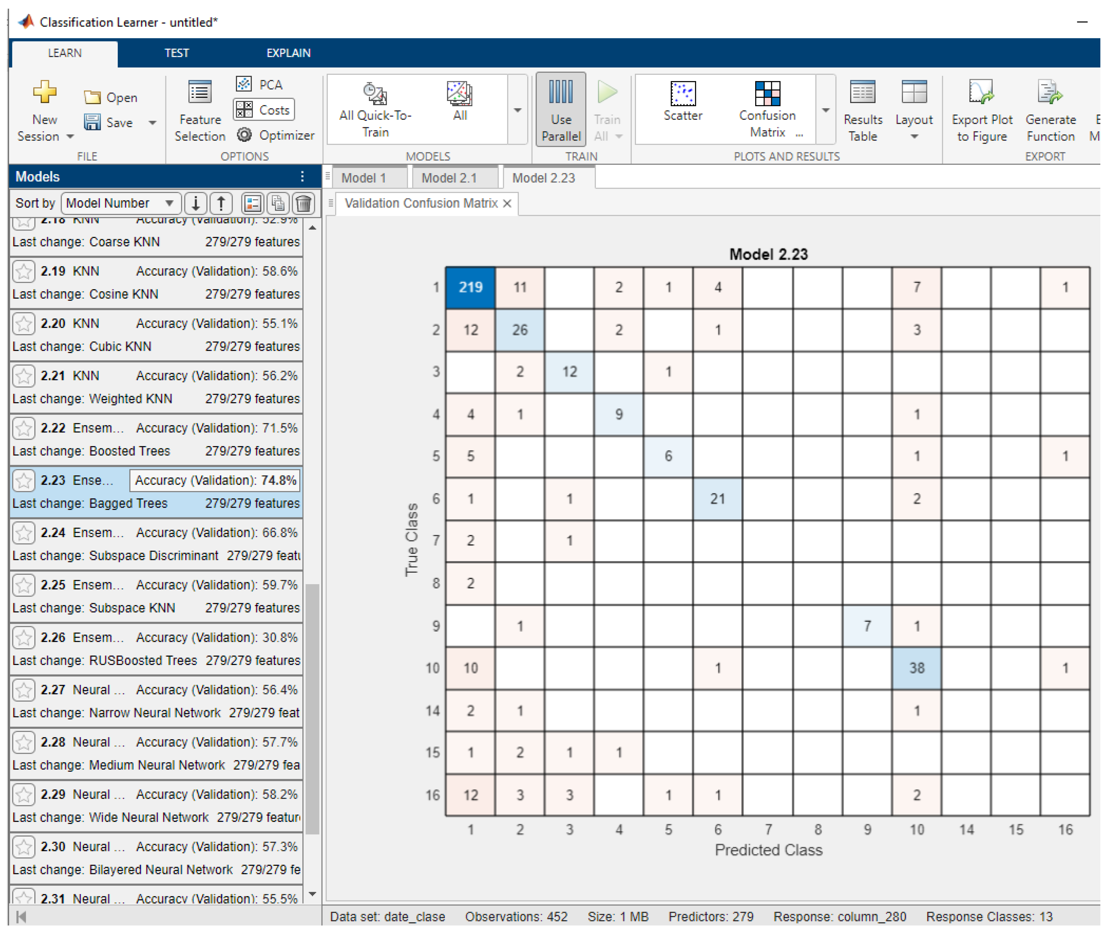
Figure 1 shows the results obtained with the arrhythmias database. It can be observed that, for the classification of the 13 classes, the best classification rate is that obtained with an ensemble of bagged trees classifiers, namely, a classification of 74.8% (for five-fold cross-validation). This database has a strongly unbalanced nature in terms of the data distribution across the 13 classes.

Table 3. Classification results for arrhythmia database with all data and feature selection results using standard methods in MATLAB Machine Learning APP.

Arrhythmia Database from UCI Machine Learning Repository [29] 452 Instances Grouped into 13 Classes, with 279 Features for Each Instance
	No. of Features	Classification Rate
Original Data OR Method of Feature Selection
ORIGINAL DATA *	279	74.8
MRMR	50	71.7
	100	74.6
	125	75
CHI2	50	73.7
	100	73.2
	150	73.9
ANOVA	50	74.8
	100	72.6
	150	74.6
KRUSKAL WALLIS *	50	75.7
	100	73
	150	75.9
LS	50	65.3
	100	69.9
	150	72
ReliefF	50	64.6
	100	69.7
	150	71.7

* The results for original data and the best results for feature selections are written in bold.

presents the classification results for the case where the most important features are selected using different feature selection methods available in the APP Machine Learning environment in MATLAB. This APP provides several methods, which have been tested on the two datasets and will be briefly presented below.

Minimum redundancy maximum relevance (MRMR) works by combining two main criteria: the maximum relevance and the minimum redundancy. Its goal is to select a subset of features that are both highly relevant to the target variable and as uncorrelated with each other as possible.

The chi-square test (CHI2) measures the independence between each feature and the target class, acting as a statistical association test.

ANOVA performs an ANOVA test for each feature to determine whether the feature values differ significantly between groups defined by the class labels. Features with p-values below a stability threshold are selected for use in the machine learning model.

The Kruskal–Wallis test is a nonparametric alternative to one-way ANOVA. Instead of using the F-statistic from classic ANOVA, the Kruskal–Wallis test employs a chi-square statistic, with the significance being determined by a p-value.

The least squares (LS) algorithm for feature selection is based on solving a system of equations by minimizing the error between the predicted and actual values (in regression problems). This algorithm is typically used in linear regression or similar methods to select the most relevant features that contribute to reducing the model error.

ReliefF (relief for feature selection) is an algorithm used for feature selection based on the importance of the features in their classification. It is an improved version of the relief algorithm, offering greater robustness in multi-class datasets.

Figure 2 exemplifies the importance of features obtained with different feature selection methods. It is found that, when applying different feature selection methods, other features are found to be relevant or their importance differs depending on the method applied.

In Table 3, it can be observed that, using all available features from the arrhythmia dataset, the best classification rate achieved with an ensemble of bagged trees classifiers using five-fold cross-validation is 74.9%. When selecting only the most relevant features, the classification rate decreases slightly, but depending on the number of selected features and the selection method, the results remain comparable or are even improved.

As seen in Table 3, using the Kruskal–Wallis method for feature selection, it is possible to achieve improved results while keeping only 50 features. For the above, this method yields the best classification results while significantly reducing the number of selected features.

If the goal is to minimize the number of selected features for classification (e.g., when hardware resources or the classification time is crucial), all tested methods prove suitable, and the classification results remain comparable to those obtained using the full dataset.

For the case of using feature selection methods based on the sparsity of the signal, methods closely related to compressed sensing and the sparse representation of a signal, the results are presented in

Table 4. Classification results for arrhythmia database for feature selection using signal sparsity-based methods.

Arrhythmia Database from UCI Machine Learning Repository [29] 452 Instances Grouped into 13 Classes, with 279 Features for Each Instance
	No. of Features	Classification Rate
ORIGINAL DATA *	279 features	74.8%
CS_RandomProjections	100 features	59.5%
Lasso	72 features	73.2%
GroupLasso	142 features	69%
OMP with no. feature setting	100 features	73.2%
BP_ADMM *	248 features	77%

* The results for original data and the best results for feature selections are written in bold.

. It is noted that the feature selection method based on the alternating direction method of multipliers (BP_ADMM) leads to improved classification results (77%) for selecting the most important 248 features. However, the LASSO, group LASSO, and OMP methods also provide classification rates comparable to the initial space. The weakest results are obtained when using random projections, which is the first part of the compressed sensing method. This first part does not involve the aspects related to the sparsity of the signal. These weaker results might also be due to the uneven distribution of data across the 13 classes.

Figure 3 exemplifies the importance of features obtained by different feature selection methods. It is found that their importance differs depending on the method applied and, by applying a threshold, relevant features are selected. The choice of threshold is an empirical matter, which depends on the database or the number of desired features.

Figure 4 shows the results obtained with oncological databases with all data using the standard classifiers from APP Machine Learning. It has been found that, using all 4000 features, a maximum classification rate of 98.6% is obtained.

Figure 5 exemplifies the importance of features obtained with different feature selection methods from the oncological databases. It is found that, for the ADMM algorithm, very few features are significant, with the importance of others being insignificant or even null. In the case of the group LASSO method, a threshold must be applied to find significant features because the algorithm fails to produce sparsity in the feature importance vector.

In

Table 5. Classification results for oncological databases with all data and feature selection obtained using standard methods in APP Machine Learning.

Oncological Databases—216 Instances Grouped into 2 Classes (Normal and Patological), with 4000 Features for Each Instance
	No. of Features	Classification Rate
ORIGINAL DATA*	4000 features	98.6%
CS_Random Projections	100 features	98.1%
Lasso	203 features	100%
GroupLasso	91 features	100%
OMP with no feature setting	400 features	100%
BP_ADMM*	107 features	100%

* The results for original data and the best results for feature selections are written in bold.

, the classifications for the oncological databases with all data obtained with feature selection using the standard methods in APP Machine Learning are shown. It has been found that, using all 4000 features, a classification rate of 98.6% is obtained. For the selection of relevant features based on the signal sparsity, improved classification rates are obtained, namely, a classification of 100%. Since the database has a large number of features, we could not perform feature selection with the standard methods in APP Machine Learning MATLAB because the computer hardware resources did not allow it. Taking into account this hardware limitation, the feature selection methods based on signal sparsity are much more efficient compared to the standard tools in MATLAB.

5. Discussion

In many cases, the data available in databases or algorithms that extract information from 1D and 2D signals or sensors are correlated with each other, often providing much less new information compared to uncorrelated data. Therefore, in such cases—especially in a classification problem where the number of available examples is small compared to the amount of information per example, and even more so when there are many classes with an uneven distribution of examples—we are faced with a complex classification problem.

For this reason, we can often achieve comparable or even improved classification rates in much less time by first applying a feature selection step. Dedicated feature selection methods exist for this purpose, falling into two main categories (due to being excessively time consuming, wrapper methods have not been considered):

(i)

Filter methods, which evaluate each feature independently of the classification model, using statistical measures to determine its relevance;

(ii)

Embedded methods, which perform feature selection during model training, simultaneously optimizing the model’s coefficients.

Filter Methods Performance

The Kruskal–Wallis method achieved the best classification rate among the tested methods, reaching 75.9% for 150 features, which is even higher than the original dataset’s performance (74.8%) using all 279 features. This indicates that removing irrelevant or redundant features can improve model accuracy. Additionally, with just 50 features, the Kruskal–Wallis test still achieved 75.7%, demonstrating its effectiveness in maintaining a strong performance with a reduced feature set.

The MRMR method, known for selecting relevant features while minimizing redundancy, achieved 75% accuracy with 125 features, comparable to the original dataset, and 74.6% with 100 features.

In contrast, the chi-square (CHI2) and ANOVA tests did not perform as well, showing a more significant performance drop when the number of features was reduced. For example:

• CHI2 with 100 features: 73.2% accuracy;
• ANOVA with 100 features: 72.6% accuracy.

Among all tested methods, the least squares (LS) and ReliefF methods performed the worst, achieving only 65.3% and 64.6% accuracy, respectively, for 50 features. Although their performance improved with more features, neither method came close to matching the performance of the full dataset.

Embedded Methods Performance

Unlike the faster but simpler filter methods, embedded methods are more advanced, relying on optimization techniques and penalized regression.

From our analysis of two datasets, the BP_ADMM method (basis pursuit using alternating direction method of multipliers) achieved the highest classification rate, reaching 77% accuracy with 248 features. This outperformed the original dataset’s performance, suggesting that careful feature selection can improve classification results.

The LASSO method, which applies L1 regularization to eliminate less relevant features, achieved 73.2% accuracy with just 72 features—very close to the original dataset’s performance but with a significantly reduced feature set. Similarly, OMP (orthogonal matching pursuit) achieved 73.2% accuracy with 100 features, indicating its ability to select an efficient subset of features.

However, the group LASSO method, which selects groups of correlated features, had a lower classification rate of 69% for 142 features.

The random projections method performed the worst, with only 59.5% accuracy, confirming that a random feature selection approach can drastically reduce model performance.

6. Conclusions

For a real and correct comparison, two essential and fundamental elements must be fulfilled, namely, (1) comparing the results using two different methods which have the same final goal and (2) using the same test and training signals. If these two essential elements are not present, the comparison is not correct. In our case, the final goal was feature selection and the databases used were the two available on the internet and MATLAB. Unfortunately, we did not find any works that use these two databases for feature selection. And comparing the classification results using a different number of features for these two bases is not correct. Therefore, in the following, we will make some comments to elucidate the difference between the methods we compared and we will point out the advantages and disadvantages of each group of methods.

These two major approaches have been analyzed in this study and the conclusions are presented below.

Filter methods are a suitable choice when a fast and simple process is needed since they analyze each feature independently of the classification model. Their main advantage is speed, as they do not require model training, making them ideal for large datasets. Additionally, being model-independent, they can be used as an initial dimensionality reduction step. However, an important disadvantage is that they do not consider interactions between features, potentially overlooking important feature combinations. Moreover, the final model’s performance may be worse compared to that obtained used more advanced methods. Thus, filter methods are useful for quickly removing irrelevant features without consuming a large amount of computational resources.

On the other hand, embedded methods offer a balance between performance and efficiency because they perform feature selection directly during the model training. Unlike filter methods, they consider interactions between features and optimize both the model and feature selection simultaneously. This makes them more precise but also slower, as they require model training. Another disadvantage is that their performance depends on the chosen algorithm, such as the LASSO regression or random forests algorithms. Additionally, they are not as exhaustive as wrapper methods, which evaluate multiple feature combinations. However, if sufficient computational resources are available, embedded methods provide a strong balance between speed and performance.

For the oncological database, all embedded methods that were tested achieved maximum classification rates, whereas the random projections method produced results similar to the original dataset.

The analysis of the two databases and feature selection by embedded methods vs. filter methods shows that appropriate feature selection plays a crucial role in machine learning-based classification. Filter methods, such as the Kruskal–Wallis and MRMR methods, can maintain or even improve the classification rate by eliminating redundant features, while more advanced methods, such as the BP_ADMM and LASSO methods, demonstrate that feature optimization can lead to superior performance. Therefore, choosing the right method depends on the analysis objective and the trade-offs between complexity, accuracy, and computational efficiency.