State of Health Prediction for Lithium-Ion Batteries Using Transformer–LSTM Fusion Model

Abstract

With the widespread use of lithium-ion batteries in various application fields, accurate prediction of battery state of health (SOH) has become an important research topic to ensure battery performance and safety. To improve the accuracy of SOH prediction, this paper proposes a novel approach that combines multidimensional feature extraction and a transformer–LSTM fusion model. This method extracts time domain, frequency domain, and time dimension features from voltage, energy, and temperature curves. It evaluates feature importance, removes redundancy, and focuses on key features most relevant to SOH. Then, using the self-attention mechanism of transformer and the long-term dependency capture ability of LSTM, an efficient fusion model is constructed to further improve the accuracy and stability of SOH prediction. The proposed method is validated based on the cycling data from 124 commercial lithium iron phosphate/graphite batteries under fast-charging conditions. Compared with existing methods, the proposed approach effectively extracts key features closely related to SOH and builds models based on these features. It achieves a prediction accuracy exceeding 50% and demonstrates superior generalization performance relative to current methods.

1. Introduction

Lithium-ion batteries are essential energy storage technologies in modern applications, renowned for their high energy density, long lifespan, and low self-discharge rate. They are increasingly used in electric vehicles and energy storage devices [1,2]. However, with long-term use, battery performance gradually degrades due to internal chemical reactions and external environmental factors, impacting its lifespan and potentially causing failure [3,4,5]. As batteries age, thermal runaway can occur, leading to rapid temperature increases that may result in combustion, posing significant safety risks [6,7]. Therefore, accurate evaluation of the SOH of lithium batteries has become a key factor in ensuring their safe and stable operation.

Battery SOH is a key indicator to measure the current health level of the battery, which reflects the performance changes and degradation of the battery during use [8,9]. SOH is usually expressed as the ratio between the current maximum available capacity of the battery and its initial rated capacity, and the calculation method is as follows:

$$\mathrm{SOH}={\displaystyle \frac{C_{max}\left(n\right)}{C\left(0\right)}}\times 100\%$$

(1)

where $C_{max}\left(n\right)$ is the maximum available capacity of the battery at the n-th charge and discharge cycle, and $C\left(0\right)$ is the initial rated capacity of the battery. As the battery is used, the maximum available capacity of the battery gradually decreases, resulting in a decrease in SOH.

The battery management system (BMS) is a crucial component of modern battery-driven devices, such as electric vehicles, battery energy storage systems, and mobile devices. Its primary responsibilities include ensuring the safety, efficiency, and long-term performance of the battery. SOH prediction plays a vital role in this [10,11]. By monitoring the battery health in real time, the BMS can provide early warning if the battery is nearing failure and detect abnormal signs of battery degradation timely, thereby effectively reducing the risk of thermal runaway and ensuring that the battery operates within a safe operating range. However, implementing SOH prediction in a BMS is challenging. First, SOH is influenced by a variety of factors, including environmental conditions like temperature and humidity, usage patterns such as charge and discharge rates and depth of discharge, material properties, and the complex changes in the internal chemical reactions of the battery, making the battery degradation process highly complex and nonlinear. This complexity makes predicting battery degradation difficult. Second, SOH prediction depends on multidimensional data, such as a battery’s charge and discharge history, voltage, current, and temperature information. In practical applications, however, the quality and uncertainty of data often pose significant challenges to achieving accurate prediction. Finally, the SOH prediction model needs robust generalization capabilities to be effective across different battery types, brands, and working conditions.

The degradation process of lithium batteries is affected by multiple factors, such as charging and discharging cycles, temperature fluctuations, and material aging. These factors cause the battery to exhibit different degradation characteristics at different stages of use and working conditions. Therefore, it is particularly important to identify key features related to battery aging. It is worth noting that the battery degradation process usually exhibits obvious nonlinear characteristics. Especially after extended use, the degradation rate tends to accelerate, which poses significant challenges to accurately predicting SOH [12,13,14].

Research on lithium battery SOH prediction can be divided into two categories: physical model-based methods and data-driven model-based methods. Physical model-based methods focus on in-depth exploration of the dynamic process of electrochemical reactions inside batteries by establishing equivalent circuits and electrochemical models of batteries. Such models usually simulate the current and voltage changes of batteries and internal chemical reactions to achieve accurate prediction of battery SOH [15,16,17,18,19,20]. For example, Rahman et al. [15] used the particle swarm optimization (PSO) algorithm to identify the key parameters of the electrochemical model of lithium batteries containing LiCoO₂ cathode materials, thereby generating corresponding battery models for healthy batteries and degraded batteries. Sung et al. [16] simplified the battery model into differential algebraic equations and used parameters such as potential, lithium-ion concentration, and lithium molar flux to calculate and solve them. Forman et al. [17] identified parameters such as anode equilibrium potential, cathode equilibrium potential, and solution conductivity based on the voltage and current-cycle data of the battery, and further established an electrochemical model for lithium-ion batteries. These electrochemical models can describe the internal electrochemical reactions of the battery with high accuracy, thereby achieving accurate prediction of the battery SOH. However, these models also have certain limitations. They usually rely on prior knowledge of battery electrochemical principles and a large amount of empirical data. In addition, the model establishment process is computationally intensive, the equations are complex, and the solutions are complicated, making them difficult to apply in actual scenarios.

With the continuous development of artificial intelligence technology, data-driven machine learning and deep-learning methods have become a hot research direction for lithium battery SOH prediction. These methods analyze various measurement data collected from the battery during operation and use machine learning and deep-learning models to extract features and make predictions. Unlike physical model-based methods, data-driven methods do not rely on prior knowledge or experience of battery electrochemical principles. Instead, they process the data obtained during the charging and discharging process to extract features related to SOH, thereby realizing the prediction of battery status [21,22,23,24,25,26]. For example, Gong et al. [24] extracted four health indicators during the charging and discharging process, established an LSTM model to map the relationship between health indicators and battery SOH, and used a particle swarm optimization algorithm to optimize the key hyperparameters of the neural network. By utilizing optimization algorithms to search for hyperparameters, the model can effectively achieve the optimal performance. However, using only four direct health indicators as input may limit the model’s generalization capabilities and the applicability of its features. Additionally, this approach may not fully leverage the potential of the model architecture, potentially hindering its ability to process more complex or diverse data. Yang et al. [25] used a convolutional neural network (CNN) to extract health indicators and SOH changes between two consecutive charging and discharging cycles, and combined it with a random forest algorithm to generate the final SOH estimate. Although CNN demonstrates robust feature extraction capabilities, the process of extracting indicators is relatively complex and cumbersome. Moreover, it is highly susceptible to noise interference, which can adversely affect the model’s stability and robustness. Furthermore, the generalization performance of the model still requires validation, potentially limiting its effectiveness and reliability in practical applications. Wei et al. [26] extracted seven health indicators from the reference discharge data of the battery and combined a deep neural network (DNN) and a Markov chain model to predict SOH. Constructing a nonlinear DNN model with multiple hidden layers effectively extracts local features from data. However, this model is susceptible to capturing random noise from the training set, which can lead to overfitting. To address this issue, a Markov chain is introduced for error correction, thereby improving prediction accuracy. While this strategy significantly enhances model performance, it also substantially increases the demand for computing resources. These methods have shown excellent prediction capabilities in experiments, indicating that extracting typical features from battery capacity decay data and establishing a mapping relationship between features and SOH are crucial for data-driven battery SOH prediction. Compared with single-feature extraction, the use of multiple-feature sets and feature combinations of different scales has been proven to be a key technology to improve model performance [27,28]. However, for batteries with different electrochemical reactions, charge and discharge curves, and ambient temperatures, the generalization ability and scope of application of existing models still need to be further verified and optimized.

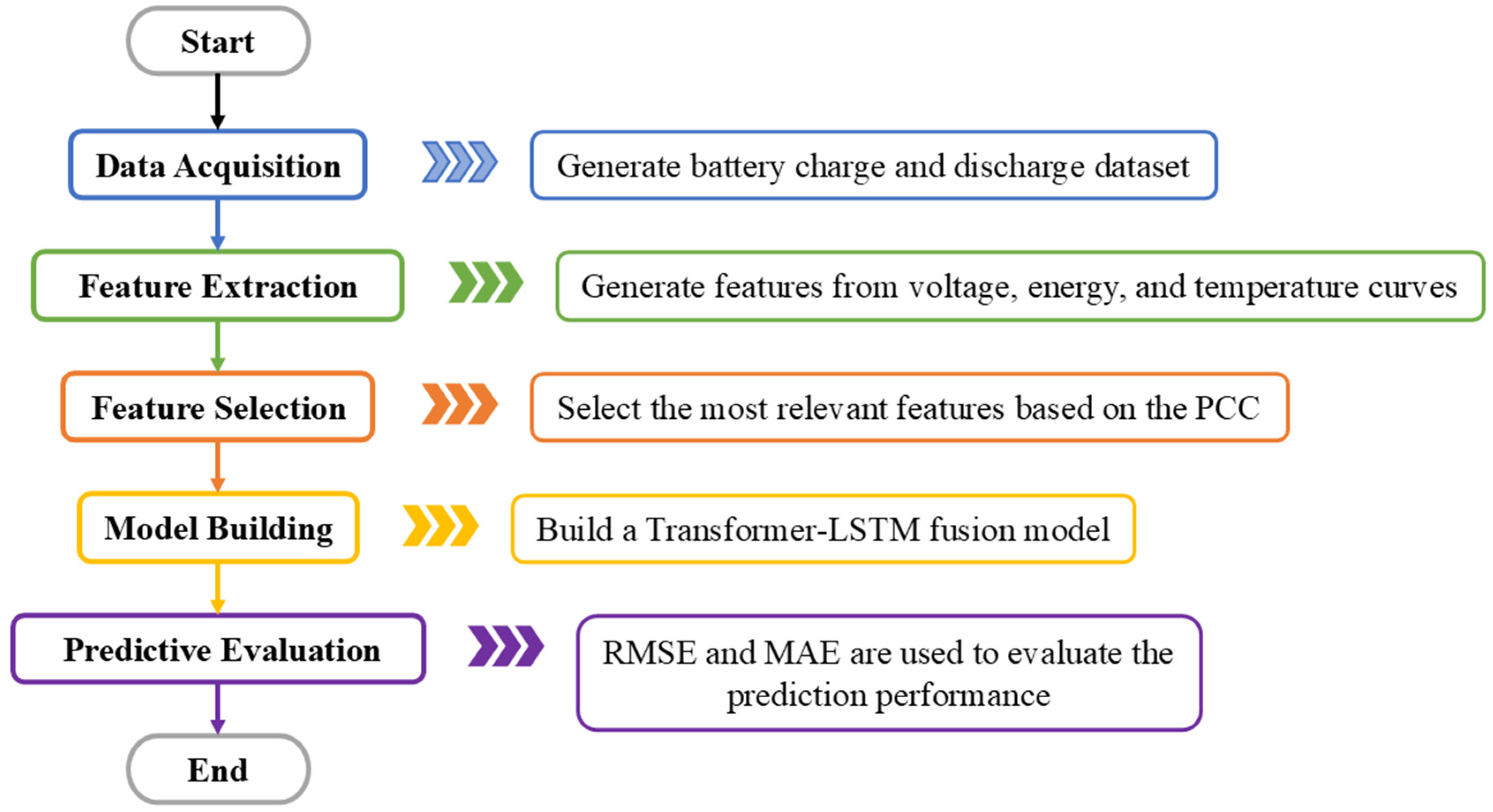
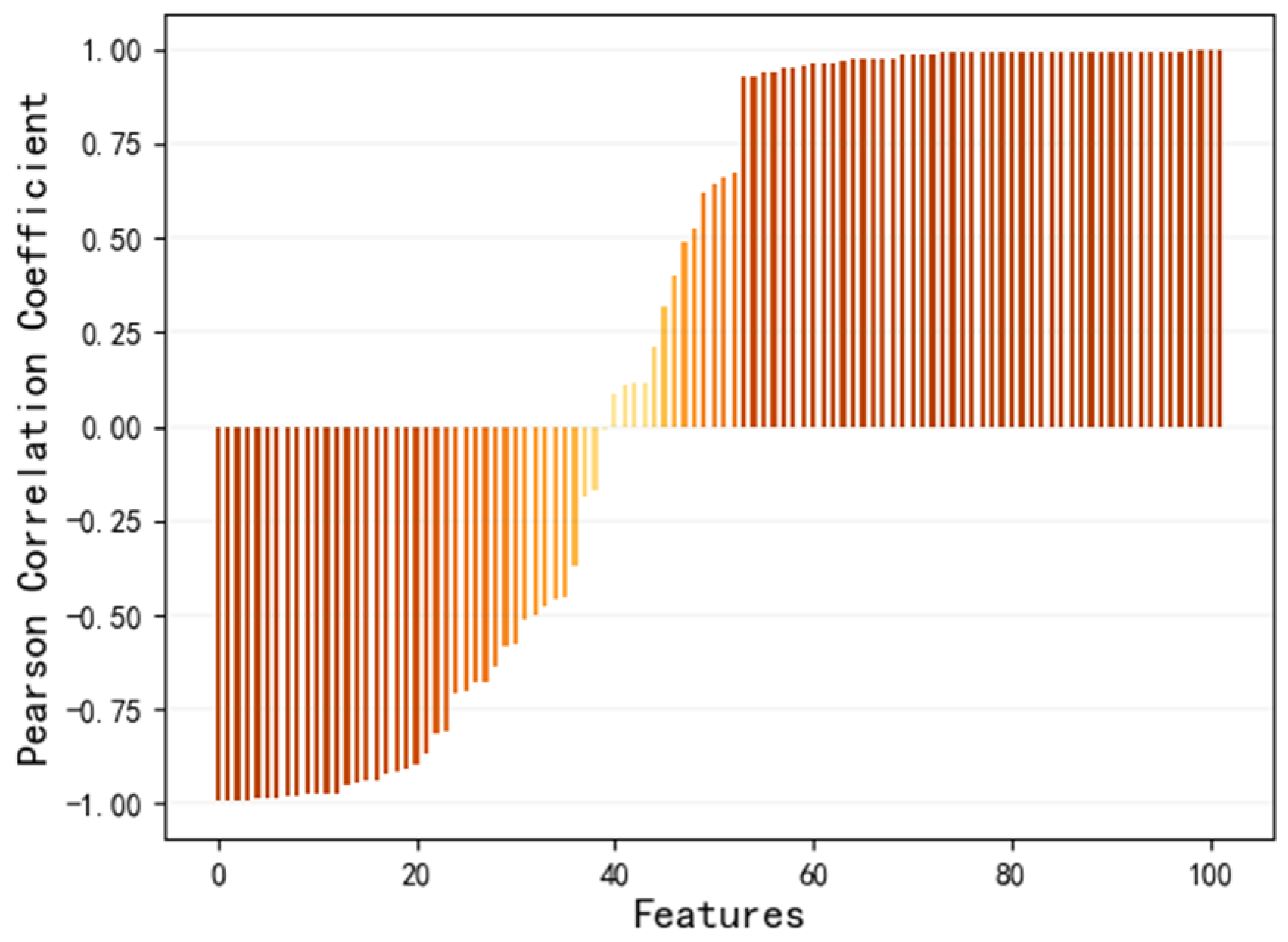
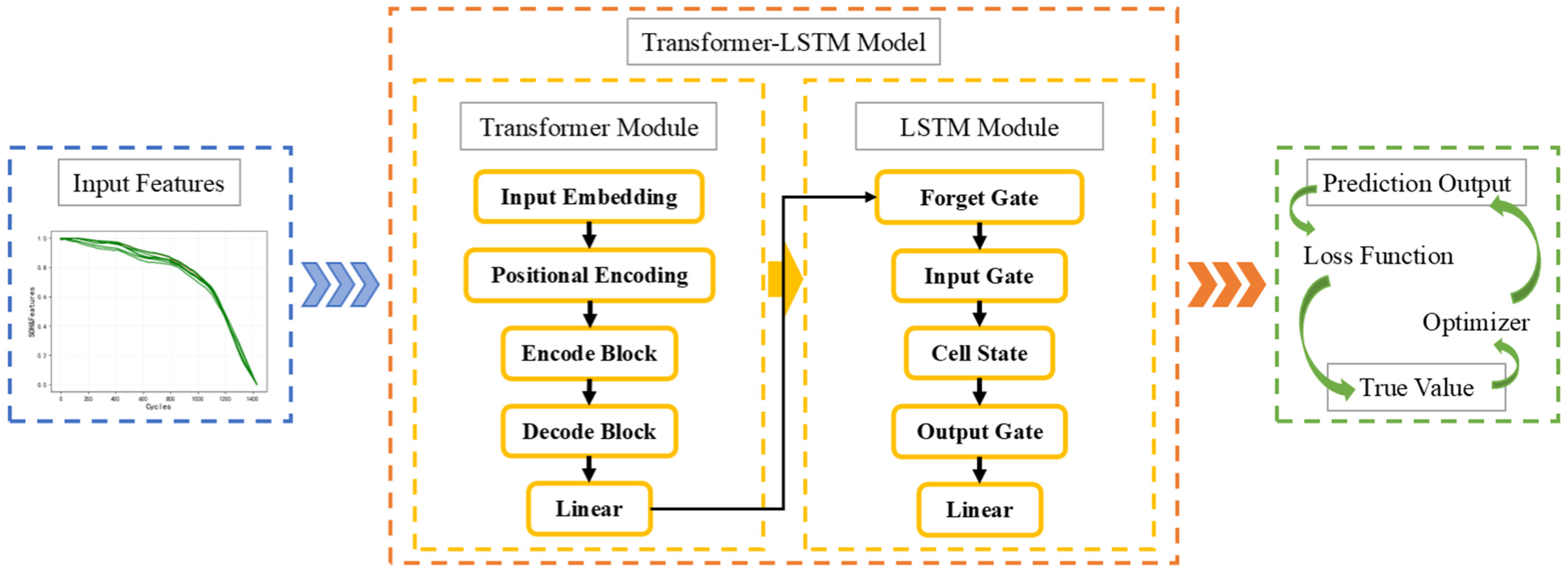
To this end, this paper proposes an innovative method based on multidimensional features and a transformer–LSTM fusion model. This method first extracts multiple features from the battery charge and discharge cycle data, including voltage, energy, and temperature curve time domain, frequency domain, and time dimension features. Subsequently, the local outlier factor (LOF) algorithm is used to identify and remove outliers in the data, and data smoothing is performed through linear interpolation and a Savitzky–Golay filter, thereby effectively improving the data quality. Next, the features most relevant to SOH are selected through correlation analysis as model input. In order to further improve the accuracy and stability of SOH prediction, we constructed a transformer–LSTM fusion model, combining the self-attention mechanism of transformer and the long-term dependency capture capability of LSTM. To verify the effectiveness of the model, we used 124 battery datasets generated under 72 different fast-charging conditions for training and testing. The experimental results indicate that the proposed model exhibits superior performance in SOH prediction and demonstrates strong generalization capability. The SOH prediction process is shown in Figure 1.

The main contributions of this paper are summarized as follows.

• A feature extraction method based on battery charge and discharge cycle data is proposed to extract the time domain, frequency domain, and time dimension characteristics of voltage, energy, and temperature curves.
• Combining an LOF algorithm, Savitzky–Golay filter, and Pearson correlation analysis, the effectiveness of the feature dataset is further improved.
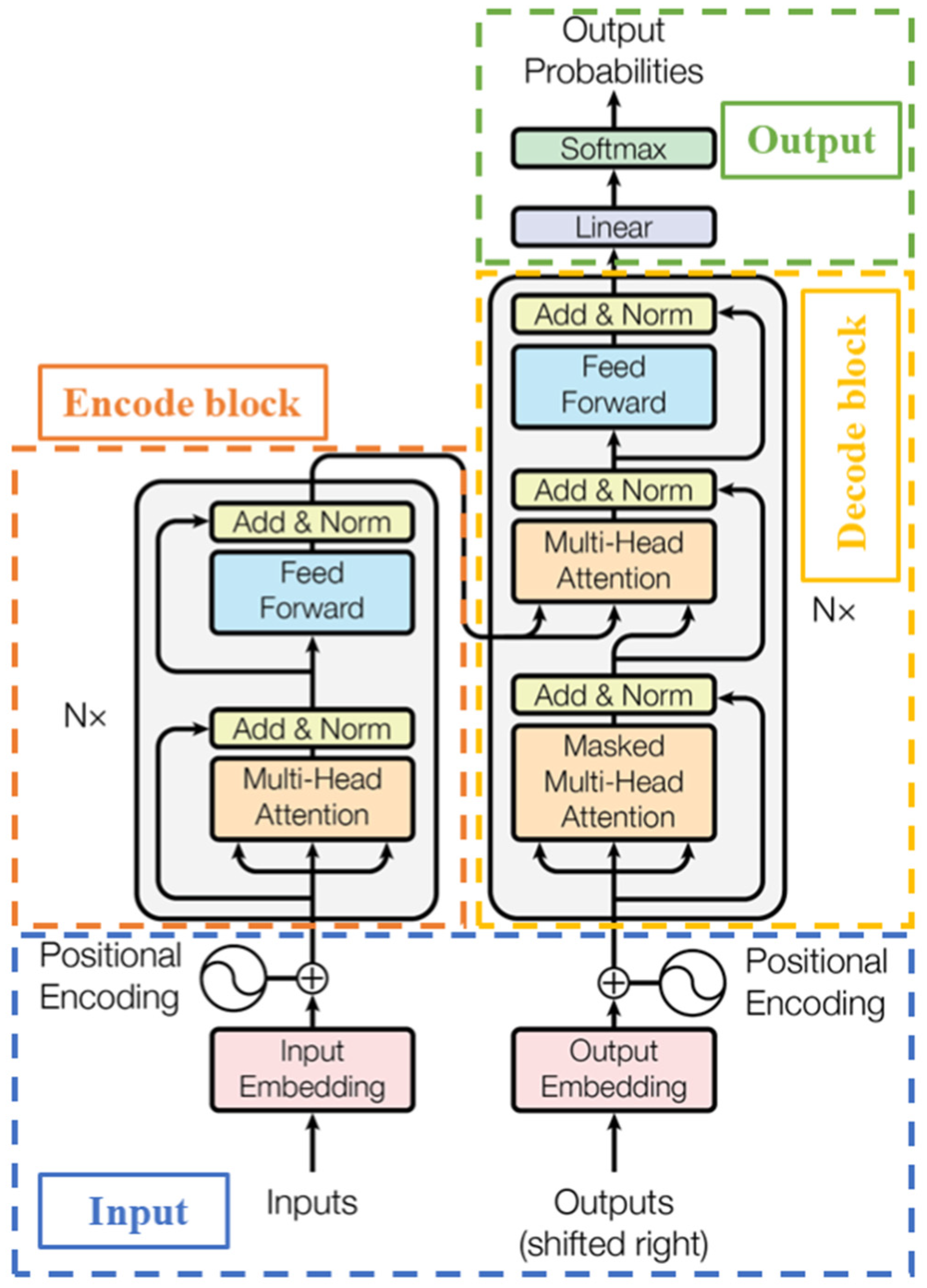
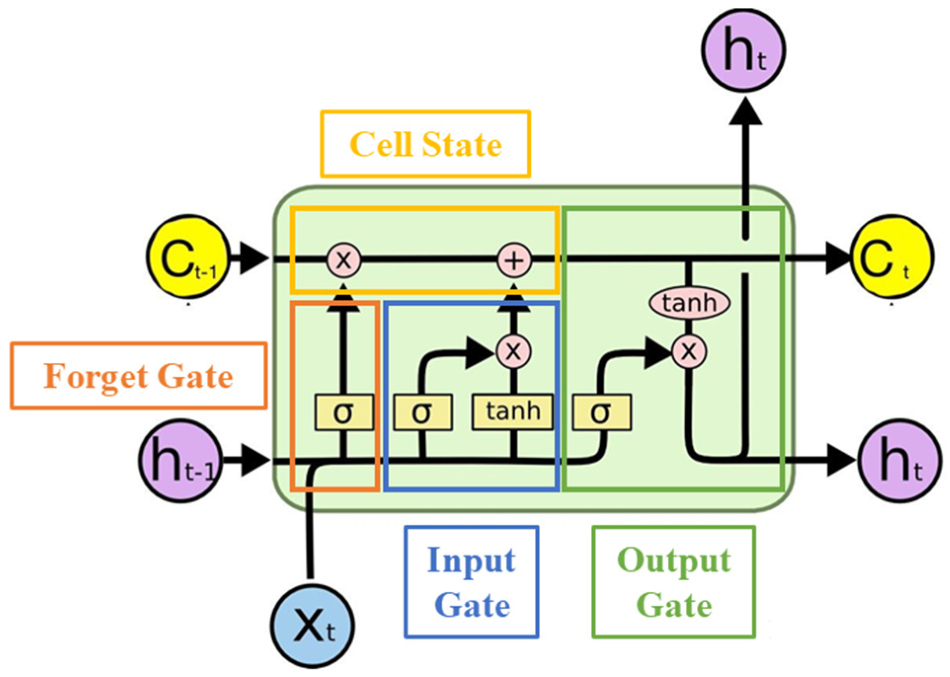
• A transformer–LSTM fusion model is built, which uses the self-attention mechanism of transformer and the long-term dependency capture capability of LSTM to improve the accuracy and stability of SOH prediction.
• Experimental results verify that the proposed method has significant SOH prediction performance, showing strong reliability and good generalizability.

2. Extraction and Selection of Multidimensional Features

Feature extraction and selection are crucial for accurate SOH prediction in lithium-ion batteries. In order to mine the key features that can effectively characterize the degree of battery aging, we extracted multidimensional data including time domain and frequency domain features of voltage, energy, temperature curves, and time dimension features from the battery’s charge and discharge cycle data. These features comprehensively represent the battery’s operating status and degradation process. However, the number of features needs to find a balance between accuracy and model complexity: too few features may lead to insufficient model prediction performance, while too many features will increase the training burden of the model. Therefore, selecting more relevant and high-information-value feature inputs can significantly improve the accuracy of SOH prediction while avoiding unnecessary complexity caused by redundant features.

2.1. Dataset

The dataset used in this paper is the MIT battery dataset, developed by Severson et al. [29] in 2019, which is the largest publicly available dataset for long-term battery degradation studies. The dataset contains 124 A123 lithium iron phosphate/graphite batteries, each with a rated capacity of 1.1 Ah (A123 Systems, Hangzhou, China). When the battery capacity decays to 80% of the rated capacity, it is considered that the battery has reached the end of its service life. All batteries are charged using 72 different multistep fast-charging strategies and discharged at a constant current in a constant-temperature chamber at 30 °C. The dataset records the long-term battery degradation process from 150 to 2300 cycles and was tested in a real physical environment, which can truly reflect the performance changes of lithium batteries in long-term use. The capacity degradation curve of the MIT dataset is shown in Figure 2.

2.2. Feature Extraction

We selectsed a charging and discharging interval from the original charge and discharge cycle data, and focuses on analyzing the changes in voltage, current, energy, and temperature in these intervals to extract features that can effectively characterize battery degradation. The variation curves for voltage, current, energy, and temperature in the charging interval during a certain cycle after normalization are shown in Figure 3a. As the number of cycles increases, the rising time of the charging voltage curve gradually shortens, and the time required to reach the cut-off voltage continues to decrease (shown in Figure 3b). The charging current curve also decreases earlier as the cycle progresses (shown in Figure 3c). At the same time, the charging energy curve shows a gradual convex trend (shown in Figure 3d); however, the charging temperature curve does not show a significant change in trend (shown in Figure 3e). These changes indicate that the information within the voltage, current, energy, and temperature curves can accurately reflect the battery’s degradation process and performance changes over time.

By analyzing these regularly changing curves, the key features reflecting battery degradation can be effectively extracted. From the original charge and discharge measurement data, we extracted the time domain, frequency domain; and time dimension features of the voltage, energy; and temperature curves, totaling 102 direct or indirect features, some of which are shown in Figure 3f. These features cover many aspects of information, including time dimension features, such as constant-current charging time and constant voltage charging time; time domain features, such as the difference, maximum slope, average value, variance, standard deviation, curve integral, root mean square value, root amplitude, skewness, kurtosis, peak factor, margin factor, pulse factor; and waveform factor of the voltage, energy; and temperature curves; and frequency domain features, such as center of gravity frequency, average frequency, frequency variance, frequency standard deviation; and frequency root mean square. These features cover the important dynamic information of batteries during the charge and discharge process, and provide solid data support for further accurate prediction of battery SOH.

2.3. Data Preprocessing

Feature curves are often affected by noise and fluctuations, resulting in outliers and uneven curves. To solve this problem, we used the LOF algorithm [30] to detect outliers effectively and replace them with linear interpolation. Additionally, the Savitzky–Golay filter [31] is applied for data smoothing to enhance feature quality. Figure 4 shows the effect of feature data after processing. In the original yellow curve, the outliers are corrected by linear interpolation and then filtered to form a smooth curve. This process effectively removes noise and abnormal fluctuations in the data and improves the quality of the feature data.

The LOF algorithm is a widely adopted technique for anomaly detection. It identifies outliers by comparing the relative density between a data point and its neighbors. If the density of a data point is significantly lower than its neighbors, the point is considered an outlier. The LOF value measures the degree of anomaly. Usually, when the LOF value of a data point is greater than 1, it indicates that the point is an outlier, and the larger the LOF value, the more likely it is to be an outlier. The calculation formula for the LOF value is as follows:

$$LOF(P)={\displaystyle \frac{1}{k}}{\sum }_{O\in N_k\left(P\right)}{\displaystyle \frac{LRD\left(P\right)}{LRD\left(O\right)}}$$

(2)

where $N_k\left(P\right)$ is the k neighbors of point P and $LRD\left(P\right)$ is the local reachability density of point P.

The Savitzky–Golay filter is a weighted average algorithm based on a moving window. It effectively smooths the curve by fitting the data points with a k-order polynomial least square in a fixed-length window. This method is particularly effective in removing random Gaussian noise.

In order to perform Gaussian filtering on the feature data, the width of the filter window is set to $w=2m+1$. Within this window, the current point in the feature data and its neighboring point set $x_m=(-m,-m+1,\cdots ,\mathrm{0,1},\cdots ,m-1,m)$ are selected. Then, a k-1-order polynomial fitting is performed using these data points, where $a_t=(\mathrm{0,1},2,\cdots ,k-1)$ represents the required polynomial parameters. Through the fitting process, the smoothed value y is generated. The calculation formula is shown below:

$$\left(\begin{array}{c}y-m\\ y-m-1\\ ...\\ y\end{array}\right)=\left(\begin{array}{c}1\\ 1\\ ⋮\\ 1\end{array}\begin{array}{c}-m\\ -m+1\\ ⋮\\ m\end{array}\begin{array}{c}\cdots \\ \cdots \\ ⋮\\ \cdots \end{array}\begin{array}{c}{\left(-m\right)}^{k-1}\\ {\left(-m+1\right)}^{k-1}\\ ⋮\\ m^{k-1}\end{array}\right)\left(\begin{array}{c}{a}_0\\ a_1\\ ⋮\\ a_{k-1}\end{array}\right)+\left(\begin{array}{c}{e}_{-m}\\ e_{-m+1}\\ ⋮\\ e_m\end{array}\right)$$

(3)

The above matrix form is written in formula form:

$$Y_{(2m+1)\times 1}=X_{(2m+1)\times k}·A_{k\times 1}+E_{(2m+1)\times 1}$$

(4)

Finally, find the least squares solution  of A and obtain the final filtered value Ŷ.

$$\begin{gathered} Ŷ=X·Â=X·\left(XT·X\right)-1·XT·Y \\ Â=(XT·X)-1·XT·Y \end{gathered}$$

(5)

2.4. Feature Selection

In order to evaluate the correlation between the extracted features and the battery SOH, we used the Pearson correlation coefficient for analysis. The Pearson correlation coefficient is a statistical indicator that measures the strength of the linear relationship between two variables. Its value range is [−1, 1], where positive values indicate positive and negative values indicate negative correlations. The closer the absolute value is to 1, the stronger the correlation. We calculated Pearson correlation coefficients between 102 features and the battery SOH, and the results are shown in Figure 5. The analysis results show a significant correlation between most features and the battery SOH, and the absolute values of the correlation coefficients of these features are close to 1, which further verifies the representativeness and effectiveness of these features. It can be seen that the extracted features can not only reflect the health status of the battery but also provide reliable input for SOH prediction. The calculation method of the Pearson correlation coefficient is shown below:

$$r={\displaystyle \frac{{\sum }_{i=1}^n(x_i-\overline{x})(y_i-\overline{y})}{\sqrt{{\sum }_{i=1}^n{(x_i-\overline{x})}^2·{\sum }_{i=1}^n{(y_i-\overline{y})}^2}}}$$

(6)

where $x_i$ and $y_i$ represent the i-th feature data point and the corresponding SOH data point, respectively, $\overline{x}$ and $\overline{y}$ are the means of the feature data and SOH data, respectively, and n is the number of feature data points.

To reduce model complexity and improve prediction accuracy, we ranked feature correlation coefficients and selected the 10 most strongly correlated features with battery SOH to extract a representative feature set, as shown in Figure 6. As can be seen from the figure, the changing trends of the SOH curve and the characteristic curve are highly similar, indicating a close correlation between these features and SOH. Especially in the degradation process, the changing pattern of the green curve can better reflect the fluctuation in the SOH curve, proving the critical role of these features in SOH prediction. These features include the time from the start of charging to the cut-off voltage of 3.6 V, the constant-current charging time, the energy in the constant-current discharge stage, the energy in the equal discharge voltage interval, the average energy in the charging stage, the energy variance in the discharge stage, the standard deviation of the energy in the discharge stage, the integral of the energy curve in the charging stage, the root mean square value of the energy in the charging stage, and the root square amplitude of the energy in the charging stage. The energy-based features are most relevant to SOH because the battery’s energy output directly reflects its storage and release capabilities, which gradually decrease as the battery ages. The energy attenuation of the battery is closely related to its internal chemical reactions and structural changes, so the energy features can effectively characterize the health of the battery. As the battery is used for a longer time, the energy loss of the battery increases. The energy features can capture this change earlier, thus becoming an indicator closely related to SOH.

3. SOH Prediction Based on Transformer–LSTM Fusion Model

Achieving reliable SOH prediction requires effectively dealing with significant inconsistencies and complex nonlinear problems in battery degradation. Battery degradation is not only influenced by various intrinsic mechanisms but is also heavily influenced by external environmental factors and operating conditions, resulting in highly uncertain degradation patterns across different batteries. In addition, as the battery life increases, the degradation rate may vary in stages or even accelerate unexpectedly, which makes the relationship between feature data and SOH complex and nonlinear. These complexities pose great challenges to a prediction model in terms of expressiveness and robustness. To tackle these challenges, this paper proposes a transformer–LSTM-based data-driven prediction method to enhance both the accuracy and robustness of SOH prediction. Figure 7 illustrates the structure of the transformer–LSTM fusion model.

3.1. Transformer–LSTM Fusion Model

Long short-term memory (LSTM) [32] is an improved version of the recurrent neural network (RNN). Introducing gating mechanisms and memory units effectively overcomes the vanishing gradient and exploding gradient problems that are common in traditional RNNs when processing long sequences. LSTM is particularly good at capturing sequence data with long-term dependencies, and has achieved remarkable results in many tasks. Transformer [33] is a neural network model based on the self-attention mechanism. With its multi-head attention mechanism and position encoding, it can fully focus on the information at each position in the sequence and is particularly suitable for sequence processing and parallel computing. Integrating LSTM with transformer leverages the strengths of both models and further improves the performance and efficiency of the model when processing sequence data.

The advantages of the transformer–LSTM model in SOH prediction are mainly reflected in its combination of the transformer’s self-attention mechanism and the LSTM’s sequence modeling capabilities [34,35,36]. First, the transformer’s self-attention mechanism can effectively focus on the contextual information in the battery degradation process and capture richer correlations between different time points. This enables the model to better understand the complex patterns in the battery degradation process, especially the changing trends at different stages of the degradation process. Second, the LSTM’s long-term dependency modeling capability can effectively capture the long-term dependencies of battery performance over time and learn the dynamic changes in battery degradation. Crucially, the combination of transformer and LSTM enables the model to consider both advantages. Transformer is good at capturing global information and parallel computing, while LSTM can effectively handle time dependencies in sequences. This complementarity helps to improve the model’s performance, especially when dealing with complex nonlinear relationships in SOH prediction. Combining the two can more comprehensively learn the deep correlations between feature data and SOH, which can effectively improve prediction accuracy and enhance the robustness of the model.

3.1.1. Transformer Module

To better understand battery degradation trends and capture contextual insights, we utilized the transformer framework, as illustrated in Figure 8. The main components of the transformer model include the input embedding layer, positional encoding, encoder, decoder, and output layer. During training, the input embedding layer first converts the input sequence into a high-dimensional vector representation. It adds positional encoding to the embedding vector to maintain each position’s relative and absolute position information in the sequence. Next, the encoder uses the self-attention mechanism to process the input features and generate context-related representations for each position, thereby capturing long-range dependencies in the sequence. The decoder combines the output of the encoder with the previous prediction results and generates the final prediction sequence through self-attention and cross-attention mechanisms. The output layer maps the decoder results to predicted values. During training, the transformer uses backpropagation to optimize the loss function and adjusts layer weights to capture complex relationships in sequence data, enhancing prediction accuracy.

In SOH prediction, transformer can effectively capture the dependencies between time steps in historical data with its self-attention mechanism. It not only focuses on local information but also fully grasps the global context, thereby accurately capturing the trend of battery degradation. In addition, transformer can process multidimensional feature data and fuse the interactions between different features through a multi-head attention mechanism to further improve the accuracy of SOH prediction. For this reason, transformer has demonstrated excellent modeling capabilities and outstanding prediction performance in battery SOH prediction.

3.1.2. LSTM Module

To better capture the trend, dynamic changes, and complex nonlinear relationships of battery performance degradation, we used the output of the transformer module as the input of the LSTM module, aiming to process battery degradation sequence data and effectively capture long-term dependencies. The LSTM model consists of a cell state, forget gate, input gate, and output gate, as shown in Figure 9. During the training process, the cell state is used as long-term memory to save the key information in the input sequence; the forget gate determines which data should be deleted from the cell state to prevent information overload; the input gate controls which new information needs to be added to the cell state and updates the memory content; the output gate determines which data to output to the next time step based on the current cell state and input information. Through this mechanism, LSTM optimizes the weights of each gate via backpropagation during training, thereby improving model’s prediction accuracy.

3.2. Optimizer and Loss Function

This article utilizes the Adam optimizer for hyperparameter tuning of the transformer–LSTM model to enhance predictive performance through minimizing the mean square error (MSE) loss function. The Adam optimizer adaptively adjusts the learning rate, combining the advantages of the momentum method and the RMSprop algorithm to render the update of each parameter more accurate and efficient. It can efficiently process high-dimensional data and accelerate convergence during training, especially for complex deep-learning models. The MSE loss function evaluates model performance by minimizing the difference between predictions and ground truth, thereby helping the model optimize and enhance prediction accuracy. The calculation formula for the MSE loss function is as follows:

$$MSE={\displaystyle \frac{1}{N}}{\sum }_{i=1}^N{(y_i-{\hat{\mathrm{y}}}_i)}^2$$

(7)

where $N$ is the total number of samples, $y_i$ is the true value of the i-th sample, and ${\hat{\mathrm{y}}}_i$ is the predicted value of the i-th sample.

4. Results and Discussion

4.1. Experimental Setup

The MIT battery dataset contains three batches of batteries, namely the “2017-05-12” batch, the “2017-06-30” batch, and the “2018-04-12” batch. According to the experimental scheme proposed by Severson et al. [29], the dataset is divided into a training set and two test sets. The training set is used for model training and parameter selection, including 20 batteries from the first batch and 21 batteries from the second batch; the test set is used to evaluate model performance, where the main test set contains 21 batteries from the first batch and 22 batteries from the second batch; and the secondary test set includes 40 batteries from the third batch. The first two batches of batteries are from the same year, constituting the training set and the main test set, and the third batch is from the batteries of the second year, serving as the secondary test set. In the experiment, the prediction results of the main test set are used to verify the accuracy of the model, while the results of the secondary test set better demonstrate the generalization ability of the model.

Based on the transformer–LSTM fusion model, we conducted three experiments on SOH prediction. In the first experiment, the degradation feature data from the same battery was divided into training set, validation set, and test set in a ratio of 4:1:5. The model was trained on the first half of the dataset to predict the SOH of the second half. The second experiment utilized the training set consisting of data from 41 batteries and selected data from one battery as the validation set. The model then performed SOH prediction on two different test sets, one consisting of 43 battery data and the other consisting of 40 battery data. The third experiment served as a comparative test to evaluate the performance of various models—LSTM, CNN–LSTM, and transformer–LSTM fusion—in SOH prediction. These experiments comprehensively assessed the predictive performance of the proposed model under diverse conditions. The experiments were conducted using Python 3.8 as the programming language and implemented with toolkits such as PyTorch 2.3.1, Scikit-learn 1.3.2, and Pandas 2.0.3.

4.2. Evaluation Indicators

We used root mean square error (RMSE) and mean absolute error (MAE) as evaluation indicators to quantify the error between the model prediction results and the actual observations to evaluate the model’s prediction performance. The definitions are as follows:

$$RMSE=\sqrt{{\displaystyle \frac{1}{n}}{\sum }_{i=1}^n{(y_i-{\hat{\mathrm{y}}}_i)}^2}$$

(8)

$$MAE={\displaystyle \frac{1}{N}}{\sum }_{i=1}^N|y_i-{\hat{\mathrm{y}}}_i|$$

(9)

where $N$ is the number of samples, $y_i$ is the actual SOH, and ${\hat{\mathrm{y}}}_i$ is the predicted SOH. Generally speaking, the smaller the values of RMSE and MAE, the higher the model’s prediction accuracy, indicating that the model’s performance is better.

4.3. Prediction on the Same Battery

In predicting the SOH of the same battery, the main challenges are twofold. On the one hand, the selected features need to be closely related to the SOH; on the other hand, the change in battery capacity usually shows a slow decline in the early stage, and as the use time increases, the SOH will enter a stage of accelerated decline along with the battery capacity. Therefore, the selection of features needs to accurately reflect the changing trends of the long-term health status of the battery. At the same time, the prediction model must adapt to the accelerated decline phase based on the training data of early capacity degradation to achieve accurate SOH prediction.

We selected two batteries from each of the batches “2017-05-12”, “2017-06-30”, and “2018-04-12” in the dataset to predict the SOH of the same battery. These batteries were those with channel numbers 18 and 20 in the “2017-05-12” batch, channel numbers 8 and 48 in the “2017-06-30” batch, and channel numbers 17 and 42 in the “2018-04-12” batch. In the dataset of each battery, we used the first half as the training set and the second half as the test set, with a ratio of 1:1 between the training set and the test set. In the SOH prediction for the same battery, selecting a small number of representative features can often bring better prediction results than using more features. However, too few features may be interfered with by noise, thus affecting the accuracy of the prediction. Finally, three key features were selected from batches “2017-05-12” and “2018-04-12”, and five key features were selected from the “2017-06-30” batch for SOH prediction.

The SOH prediction results for the same battery are shown in Figure 10. It can be observed that the SOH value (blue curve) in the first half shows a slow decay trend, while in the second half, the rate of decline of SOH is significantly accelerated. Using the first-half data to predict the second half, although a noticeable deviation exists between the predicted and true values towards the end of the prediction, the results indicate that the trend between the predicted values (red curve) and the true values is largely consistent. According to the prediction evaluation indicators shown in

Table 1. Prediction evaluation indicators on the same battery.

Battery	RMSE	MAE
2017-05-12_18	0.00509	0.00338
2017-05-12_20	0.00329	0.00272
2017-06-30_8	0.00984	0.00621
2017-06-30_48	0.00392	0.00185
2018-04-12_17	0.00231	0.00163
2018-04-12_42	0.00205	0.00189

, the RMSE values of the six batteries are between 0.00205 and 0.00984 and the MAE values are between 0.00163 and 0.00621. These data show that although the prediction errors of batteries in different batches are different, overall, the model has high accuracy in SOH prediction. In particular, the battery with channel number 42 in the “2018-04-12” batch has a very small prediction error, which is consistent with the results in Figure 10. This shows that the features selected based on the transformer–LSTM prediction model can accurately capture the changing patterns of battery SOH, verifying the effectiveness and accuracy of the selected features and models in battery SOH prediction.

4.4. Prediction of the Different Batteries

Predicting the SOH of different batteries presents two main challenges: feature selection effectiveness and model generalization capability. First, whether the selected features effectively reflect changes in SOH directly impacts prediction accuracy. Therefore, selected features must strongly correlate with the battery’s degradation process and be representative enough to capture the dynamics of its SOH. Second, the model’s generalization ability is of critical importance. Factors such as operating environment and cycle conditions may lead to varying performance across batteries during SOH degradation. Thus, the prediction model must generalize well, adapt to the characteristics of different batteries, and accurately infer their SOH trends.

For different batteries, we used the training set and two test sets in Section 4.1 for SOH prediction. The training set contains the complete feature data of 41 batteries from the first two batches, and the test set is divided into the primary test set (containing 43 batteries) and the secondary test set (containing 40 batteries). In order to ensure the representativeness of the features while avoiding increasing the computational burden of the model, we chose to predict battery SOH based on 10 features. In the two test sets, six batteries were randomly selected for prediction performance evaluation: batteries with channel numbers 27 and 36 from the “2017-05-12” batch, batteries with channel numbers 11 and 17 from the “2017-06-30” batch, and batteries with channel numbers 20 and 30 from the “2018-04-12” batch.

The SOH prediction results for different batteries are shown in Figure 11. Although the cycles of different batteries vary from 463 to 874, their SOH change trends show similar decay patterns. Even so, the model demonstrates excellent predictive performance on the test set. The predicted value (red curve) is highly consistent with the true value (blue curve), especially in the critical stage of battery decay, and the prediction model can accurately capture the change in SOH. In particular, for the battery with channel number 36 in the batch “2017-05-12” and the battery with channel number 20 in the batch “2018-04-12”, the predicted RMSE and MAE values are both less than 0.002, as shown in

Table 2. Prediction evaluation indicators on the different batteries.

Battery	RMSE	MAE
2017-05-12_27	0.00339	0.00275
2017-05-12_36	0.00159	0.00124
2017-06-30_11	0.00487	0.00394
2017-06-30_17	0.00341	0.00248
2018-04-12_20	0.00134	0.00099
2018-04-12_30	0.00329	0.00192

, showing extremely low prediction errors and the high-precision prediction ability of the model on these batteries. For the battery with channel number 17 in the batch “2017-06-30”, the figure shows that the SOH is interfered with by noise, but the model can still accurately reflect the overall decay trend of the battery. As for the battery with channel number 30 in the batch of “2018-04-12”, unlike other batteries, its SOH maintained a similar downward trend throughout the cycle. Although there was a certain deviation between the predicted value and the true value at the beginning and end of the data, the overall performance remained consistent. These results show that the model performs stably on different batteries and can effectively handle the complexity and differences in battery SOH prediction.

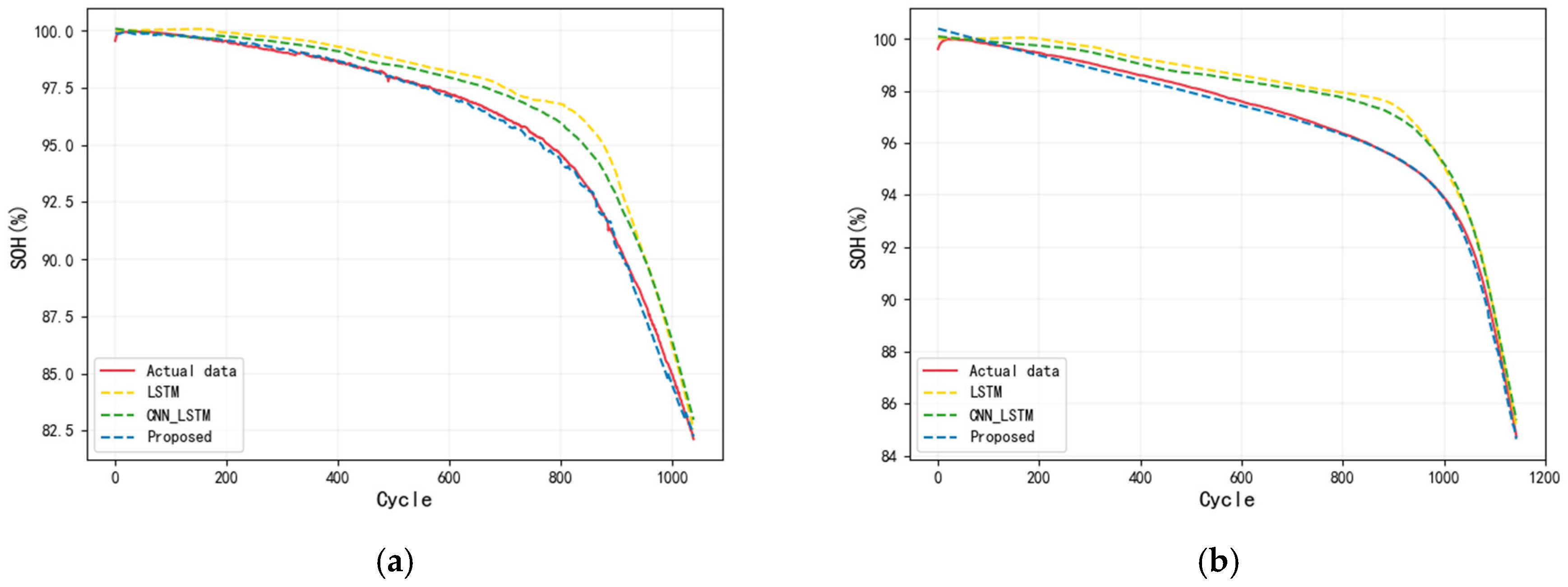
4.5. Comparative Experiments

To verify the effectiveness of the proposed method in battery SOH prediction, we compared the performance of three models: LSTM, CNN–LSTM, and transformer–LSTM. For the experiments, we selected the battery with channel number 44 in the batch “2017-05-12” and the battery with channel number 48 in the batch “2018-04-12” for testing, and the prediction results displayed in Figure 12. The prediction accuracy metrics of each model, including RMSE and MAE, are documented in

Table 3. Prediction evaluation indicators based on different methods.

Methods	2017-05-12_44		2018-04-12_48
	RMSE	MAE	RMSE	MAE
LSTM	0.01325	0.01064	0.01034	0.00900
CNN–LSTM	0.00976	0.00768	0.00877	0.00739
Proposed	0.00209	0.00151	0.00180	0.00144

. The results indicate that the proposed method excels in the SOH prediction task, achieving significantly lower prediction errors compared to other models. Specifically, while the LSTM model is adept at capturing long-term dependencies, it falls short in terms of prediction accuracy. The CNN–LSTM model has an advantage in extracting local spatial features from the input data; however, the transformer–LSTM model outperforms the others in terms of prediction accuracy and generalization capability. These results clearly highlight the significant advantages of the proposed method in terms of prediction accuracy and generalization performance.

4.6. Generalization Performance

In Section 4.3, SOH prediction for the same battery demonstrates that the sizes of the training and test sets are uneven due to the varying end-of-life cycles of each battery, which partially evaluates the model’s generalization capability. Despite these differences, the model demonstrates its generalization capability by predicting the battery’s SOH changes with reasonable accuracy. In Section 4.4, the training set is constructed using batteries from different batches, which further improves the generalization ability of the model. In particular, the data of the “2018-04-12” batch is used as a secondary dataset. This batch is one year apart and uses different batteries for prediction. As shown in

Table 4. Prediction results of the transformer–LSTM model on two test sets.

Test Set	RMSE	MAE
Primary test set	0.00711	0.00557
Secondary test set	0.00785	0.00706

, the average RMSE and MAE values predicted by the model on the two test sets are shown. The results thoroughly verify the adaptability and robustness of the model when facing different batteries, and further prove that prediction ability based on the transformer–LSTM model can still be stable under different batteries and different usage cycles.

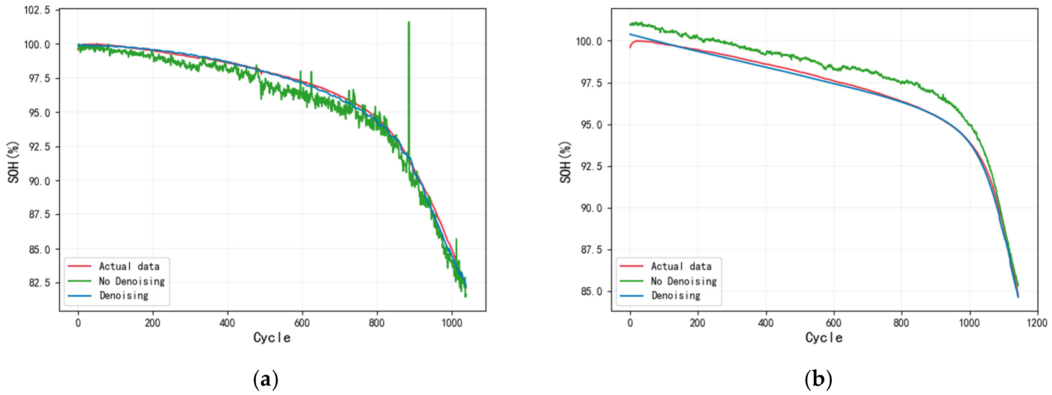
4.7. Ablation Experiment

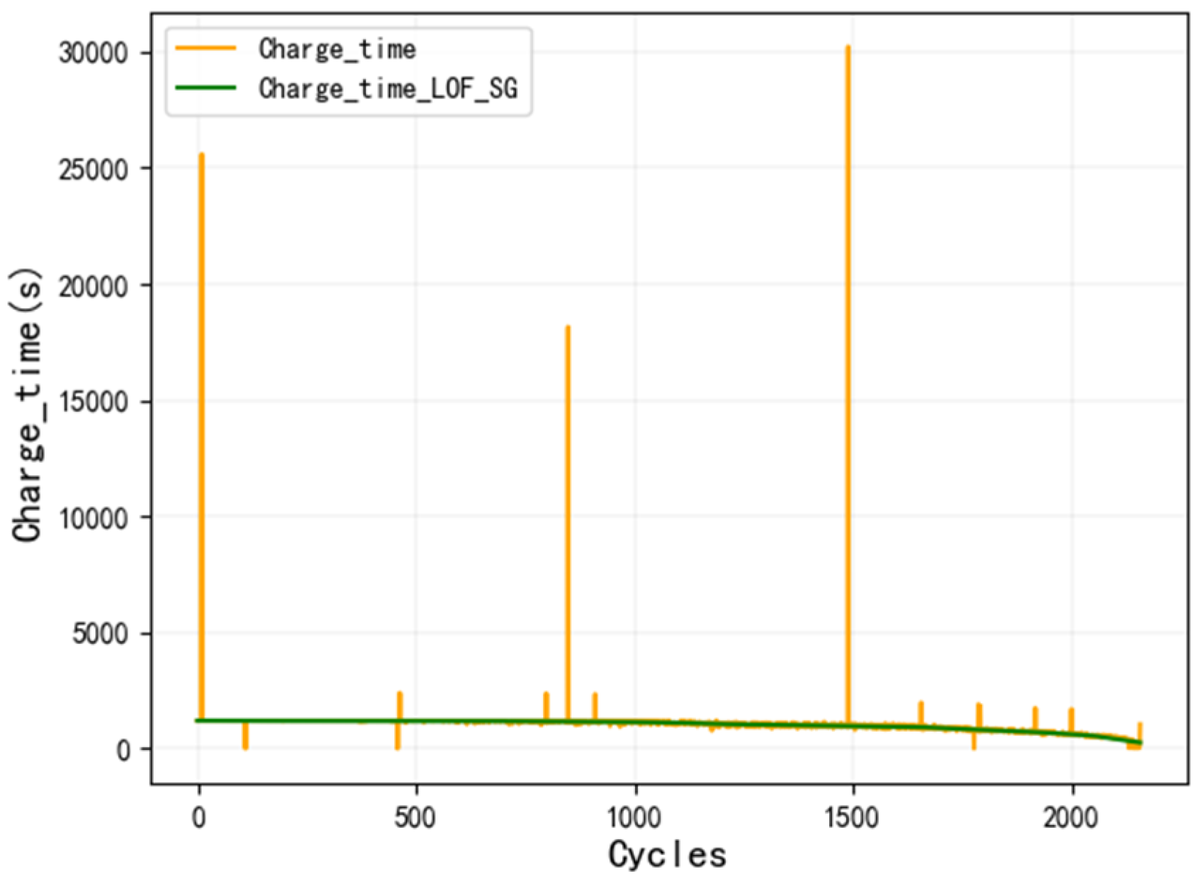
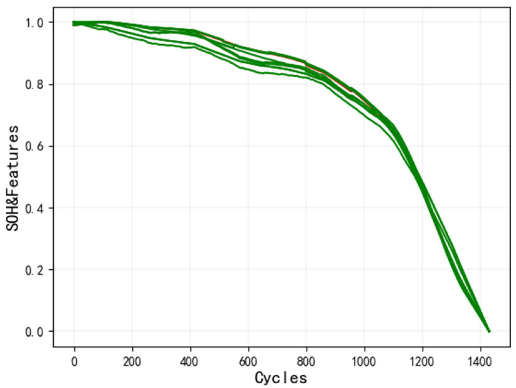
We thoroughly investigated the noise level within the dataset and its effects on the prediction accuracy and model robustness of SOH. As illustrated in Figure 4, there are some outliers in the dataset that are obviously deviant, and some of them are far from the overall data curve. If the curve containing these outliers is directly normalized and correlated, these features are obviously unable to effectively characterize SOH. Through experiments, it was found that there were notable differences between the features after noise removal and the features selected for the non-denoised data. Although the features selected for the non-denoised data retained some capacity to characterize SOH, their prediction performance was considerably inferior, as depicted in Figure 13. Compared with the prediction results after denoising, the prediction error of the non-denoised model is larger, the prediction curve appears to be more unsmooth, and abnormal prediction values appear. These findings underscore the substantial negative impact of noise on prediction performance, highlighting that denoising significantly enhances the model’s prediction accuracy.

5. Conclusions

This paper proposes a method for predicting battery SOH based on multidimensional features and a transformer–LSTM fusion model, aiming to enhance the accuracy and generalizability of SOH prediction. The key findings reveal that by extracting features from the time domain, frequency domain, and time dimension of the voltage, energy and temperature curves, the trend of battery degradation can be effectively captured. Furthermore, denoising the feature data significantly improves prediction accuracy and reduces the negative impact of noise on model performance. By integrating these optimized features with the transformer–LSTM fusion model for prediction, the experimental results demonstrate that the proposed model excels in both prediction accuracy and generalization ability, thus verifying its efficacy and practicality in SOH prediction.

Looking ahead, this study will focus further on the implementation and optimization of SOH prediction in actual application scenarios. Compared to laboratory scenarios, the operating conditions of actual batteries are considerably more complex and variable. They are influenced by unstable external factors such as fluctuations in ambient temperature, variations in user operating habits, and the use of diverse charging equipment. These factors pose challenges to the accuracy of SOH prediction. Therefore, to ensure effective implementation of SOH prediction in real-world applications, it is crucial to adapt and optimize the model based on actual operating data of the batteries to accommodate changes in real-life scenarios.

References

1. Che, Y.; Deng, Z.; Lin, X.; Hu, L.; Hu, X. Predictive battery health management with transfer learning and online model correction. IEEE Trans. Veh. Technol. 2021, 70, 1269–1277. [Google Scholar] [CrossRef]
2. Hu, X.; Feng, F.; Liu, K.; Zhang, L.; Xie, J.; Liu, B. State estimation for advanced battery management: Key challenges and future trends. Renew. Sustain. Energy Rev. 2019, 114, 109334. [Google Scholar] [CrossRef]
3. Hu, X.; Xu, L.; Lin, X.; Pecht, M. Battery lifetime prognostics. Joule 2020, 4, 310–346. [Google Scholar] [CrossRef]
4. Li, X.; Wang, Z.; Zhang, L.; Zou, C.; Dorrell, D.D. State-of-health estimation for Li-ion batteries by combing the incremental capacity analysis method with grey relational analysis. J. Power Sources 2019, 410, 106–114. [Google Scholar] [CrossRef]
5. Berecibar, M.; Gandiaga, I.; Villarreal, I.; Omar, N.; Van Mierlo, J.; Van den Bossche, P. Critical review of state of health estimation methods of Li-ion batteries for real applications. Renew. Sustain. Energy Rev. 2016, 56, 572–587. [Google Scholar] [CrossRef]
6. Opitz, A.; Badami, P.; Shen, L.; Vignarooban, K.; Kannan, A.M. Can Li-Ion batteries be the panacea for automotive applications? Renew. Sustain. Energy Rev. 2017, 68, 685–692. [Google Scholar] [CrossRef]
7. Feng, X.; Ouyang, M.; Liu, X.; Lu, L.; Xia, Y.; He, X. Thermal runaway mechanism of lithium ion battery for electric vehicles: A review. Energy Storage Mater. 2018, 10, 246–267. [Google Scholar] [CrossRef]
8. Zheng, L.; Zhang, L.; Zhu, J.; Wang, G.; Jiang, J. Co-estimation of state-of-charge, capacity and resistance for lithium-ion batteries based on a high-fidelity electrochemical model. Appl. Energy 2016, 180, 424–434. [Google Scholar] [CrossRef]
9. Ungurean, L.; Cârstoiu, G.; Micea, M.V.; Groza, V. Battery state of health estimation: A structured review of models, methods and commercial devices. Int. J. Energy Res. 2017, 41, 151–181. [Google Scholar] [CrossRef]
10. Lipu, M.H.; Hannan, M.A.; Hussain, A.; Hoque, M.; Ker, P.J.; Saad, M.H.M.; Ayob, A. A review of state of health and remaining useful life estimation methods for lithium-ion battery in electric vehicles: Challenges and recommendations. J. Clean. Prod. 2018, 205, 115–133. [Google Scholar] [CrossRef]
11. Khan, S.; Yairi, T. A review on the application of deep learning in system health management. Mech. Syst. Signal Process. 2018, 107, 241–265. [Google Scholar] [CrossRef]
12. He, W.; Li, Z.; Liu, T.; Liu, Z.; Guo, X.; Du, J.; Li, X.; Sun, P.; Ming, W. Research progress and application of deep learning in remaining useful life, state of health and battery thermal management of lithium batteries. J. Energy Storage 2023, 70, 107868. [Google Scholar] [CrossRef]
13. Khaleghi, S.; Hosen, M.S.; Van Mierlo, J.; Berecibar, M. Towards machine-learning driven prognostics and health management of Li-ion batteries. A comprehensive review. Renew. Sustain. Energy Rev. 2024, 192, 114224. [Google Scholar] [CrossRef]
14. Kim, E.; Kim, M.; Kim, J.; Kim, J.; Park, J.-H.; Kim, K.-T.; Park, J.-H.; Kim, T.; Min, K. Data-driven methods for predicting the state of health, state of charge, and remaining useful life of li-ion batteries: A comprehensive review. Int. J. Precis. Eng. Manuf. 2023, 24, 1281–1304. [Google Scholar] [CrossRef]
15. Rahman, M.A.; Anwar, S.; Izadian, A. Electrochemical model parameter identification of a lithium-ion battery using particle swarm optimization method. J. Power Sources 2016, 307, 86–97. [Google Scholar] [CrossRef]
16. Sung, W.; Shin, C.B. Electrochemical model of a lithium-ion battery implemented into an automotive battery management system. Comput. Chem. Eng. 2015, 76, 87–97. [Google Scholar] [CrossRef]
17. Forman, J.C.; Moura, S.J.; Stein, J.L.; Fathy, H.K. Genetic parameter identification of the doyle-fuller-newman model from experimental cycling of a lifepo 4 battery. In Proceedings of the 2011 American Control Conference, San Francisco, CA, USA, 29 June–1 July 2011. [Google Scholar] [CrossRef]
18. Kim, J.-K.; Lee, C.-S. Co-simulation approach for analyzing electric-thermal interaction phenomena in lithium-ion battery. Int. J. Precis. Eng. Manuf.-Green Technol. 2015, 2, 255–262. [Google Scholar] [CrossRef]
19. Tian, N.; Wang, Y.; Chen, J.; Fang, H. One-shot parameter identification of the Thevenin’s model for batteries: Methods and validation. J. Energy Storage 2020, 29, 101282. [Google Scholar] [CrossRef]
20. Chin, C.S.; Gao, Z.; Zhang, C.Z. Comprehensive electro-thermal model of 26,650 lithium battery for discharge cycle under parametric and temperature variations. J. Energy Storage 2020, 28, 101222. [Google Scholar] [CrossRef]
21. Kim, S.W.; Kong, J.H.; Lee, S.W.; Lee, S. Recent advances of artificial intelligence in manufacturing industrial sectors: A review. Int. J. Precis. Eng. Manuf. 2022, 23, 111–129. [Google Scholar] [CrossRef]
22. Cho, S.; Seo, H.; Lee, G.; Choi, S.; Choi, H. A rapid learning model based on selected frequency range spectral subtraction for the data-driven fault diagnosis of manufacturing systems. Int. J. Precis. Eng. Manuf.-Smart Technol. 2023, 1, 49–62. [Google Scholar] [CrossRef]
23. Park, H.J.; Kim, S.; Han, S.-Y.; Ham, S.; Park, K.J.; Choi, J.-H. Machine health assessment based on an anomaly indicator using a generative adversarial network. Int. J. Precis. Eng. Manuf. 2021, 22, 1113–1124. [Google Scholar] [CrossRef]
24. Gong, Y.; Zhang, X.; Gao, D.; Li, H.; Yan, L.; Peng, J.; Huang, Z. State-of-health estimation of lithium-ion batteries based on improved long short-term memory algorithm. J. Energy Storage 2022, 53, 105046. [Google Scholar] [CrossRef]
25. Yang, N.; Song, Z.; Hofmann, H.; Sun, J. Robust State of Health estimation of lithium-ion batteries using convolutional neural network and random forest. J. Energy Storage 2022, 48, 103857. [Google Scholar] [CrossRef]
26. Wei, Z.; Han, X.; Li, J. State of health assessment for echelon utilization batteries based on deep neural network learning with error correction. J. Energy Storage 2022, 51, 104428. [Google Scholar] [CrossRef]
27. Zhang, M.; Yin, J.; Chen, W. SOH estimation and RUL prediction of lithium batteries based on multidomain feature fusion and CatBoost model. Energy Sci. Eng. 2023, 11, 3082–3101. [Google Scholar] [CrossRef]
28. Khaleghi, S.; Firouz, Y.; Van Mierlo, J.; Van Den Bossche, P. Developing a real-time data-driven battery health diagnosis method, using time and frequency domain condition indicators. Appl. Energy 2019, 255, 113813. [Google Scholar] [CrossRef]
29. Severson, K.A.; Attia, P.M.; Jin, N.; Perkins, N.; Jiang, B.; Yang, Z.; Chen, M.H.; Aykol, M.; Herring, P.K.; Fraggedakis, D. Data-driven prediction of battery cycle life before capacity degradation. Nat. Energy 2019, 4, 383–391. [Google Scholar] [CrossRef]
30. Breunig, M.M.; Kriegel, H.-P.; Ng, R.T.; Sander, J. LOF: Identifying density-based local outliers. In Proceedings of the 2000 ACM SIGMOD International Conference on Management of Data, Dallas, TX, USA, 16–18 May 2000. [Google Scholar] [CrossRef]
31. Kowalski, P.; Smyk, R. Review and comparison of smoothing algorithms for one-dimensional data noise reduction. In Proceedings of the 2018 International Interdisciplinary PhD Workshop (IIPhDW), Swinoujscie, Poland, 9–12 May 2018. [Google Scholar] [CrossRef]
32. Hochreiter, S.; Schmidhuber, J. Long short-term memory. Neural Comput. 1997, 9, 1735–1780. [Google Scholar] [CrossRef]
33. Vaswani, A.; Shazeer, N.; Parmar, N.; Uszkoreit, J.; Jones, L.; Gomez, A.N.; Kaiser, Ł.; Polosukhin, I. Attention is all you need. arXiv 2017. [Google Scholar] [CrossRef]
34. Cao, K.; Zhang, T.; Huang, J. Advanced hybrid LSTM-transformer architecture for real-time multi-task prediction in engineering systems. Sci. Rep. 2024, 14, 4890. [Google Scholar] [CrossRef]
35. Shi, J.; Wang, S.; Qu, P.; Shao, J. Time series prediction model using LSTM-Transformer neural network for mine water inflow. Sci. Rep. 2024, 14, 18284. [Google Scholar] [CrossRef]
36. Xie, D.; Liu, Z.; Wang, F.; Song, Z. A transformer and LSTM-based approach for blind well lithology prediction. Symmetry 2024, 16, 616. [Google Scholar] [CrossRef]
Figure 1. Flowchart for SOH prediction.
Applsci 15 03747 g001
Figure 2. Lithium battery capacity–degradation curve of MIT dataset.
Applsci 15 03747 g002
Figure 3. (a) Variation curves of voltage, current, energy, and temperature within the charging range; (b) charging voltage curves under different cycles; (c) charging current curves under different cycles; (d) charging energy curves under different cycles; (e) charging temperature curves under different cycles; (f) comparison of SOH (red curve) and multidimensional features generated by voltage, current, energy; and temperature curves (green curve).
Applsci 15 03747 g003
Figure 4. Data smoothing using the LOF algorithm and Savitzky–Golay filter.
Applsci 15 03747 g004
Figure 5. Pearson correlation coefficients between SOH and features.
Applsci 15 03747 g005
Figure 6. Comparison of SOH (red curve) with the 10 most strongly correlated features (green curve).
Applsci 15 03747 g006
Figure 7. The structure of the transformer–LSTM fusion model.
Applsci 15 03747 g007
Figure 8. The structure of the transformer model.
Applsci 15 03747 g008
Figure 9. The structure of the LSTM model.
Applsci 15 03747 g009
Figure 10. (a) Prediction results for battery with batch number 18 on “2017-05-12”, (b) prediction results for battery with batch number 20 on “2017-05-12”, (c) prediction results for battery with batch number 8 on “2017-06-30”, (d) prediction results for battery with batch number 48 on “2017-06-30”, (e) prediction results for battery with batch number 17 on “2018-04-12”, (f) prediction results for battery with batch number 42 on “2018-04-12”.
Applsci 15 03747 g010
Figure 11. (a) Prediction results for battery with batch number 27 on “2017-05-12”, (b) prediction results for battery with batch number 36 on “2017-05-12”, (c) prediction results for battery with batch number 11 on “2017-06-30”, (d) prediction results for battery with batch number 17 on “2017-06-30”, (e) prediction results for battery with batch number 20 on “2018-04-12”, (f) prediction results for battery with batch number 30 on “2018-04-12”.
Applsci 15 03747 g011
Figure 12. (a) Prediction results for battery with batch number 44 on “2017-05-12”, (b) prediction results for battery with batch number 48 on “2018-04-12”.
Applsci 15 03747 g012
Figure 13. (a) Prediction results for battery with batch number 44 on “2017-05-12”, (b) prediction results for battery with batch number 48 on “2018-04-12”.
Applsci 15 03747 g013