Monitorization of Cleaning Processes from Digital Video Spatiotemporal Analysis: Cleaning Kinetics from Characteristic Times

Abstract

The cleaning process kinetics of metallic surfaces has been studied by means of digital video monitoring. Two theoretical models based on experimental observations are proposed for two possible cleaning kinetics mechanisms and two practical cases that can be adapted to these models are analyzed. As a kinetic parameter, the duration of the cleaning of a metallic surface is defined from the time evolution of the color intensities and their variance. These times allow us to characterize and to optimize the cleaning process procedure. Apparent activation energies are estimated from the characteristic times at different temperatures.

1. Introduction

In the chemical and food industries, metallic materials are commonly used to build tanks, reservoirs and pipes that connect them due to their high mechanical strength, good sealing and high durability. A notable benefit of these materials is their capacity to withstand elevated temperatures and pressures, which renders them more suitable for use in harsh working conditions that would be impractical with alternative, less expensive materials. However, it should be noted that metallic materials are also susceptible to degradation and alterations in properties over time, a consequence of the continuous exposure of metallic surfaces to chemical or foodstuffs [1,2,3,4,5,6,7,8,9,10,11].

Among many potential metallic alterations, corrosion must be controlled since it generates important losses. Degradation of the material and formation of oxides or hydroxides layers results in a loss of thermal conductivity (of special relevance in boilers and heat exchangers) or in the contamination of final products, which can lead to a reduction in quality in the chemical industry or to food safety problems in the food industry. Calcareous (calcium carbonate) deposits, for example, manifest on the metal surfaces of systems when hard water is employed. This phenomenon is accelerated at elevated temperatures (over 45 °C). To solve these problems, it is common to pre-treat the circulating water, employing additives that impede the precipitation of salts or cleaning with acidic products once the scaling layer has already been formed. In the food industry, the circulation and storage of organic matter facilitates the formation and growth of microorganisms that can form biological colonies, or so-called biofilms [12,13,14,15,16,17,18,19,20,21]. These biofilms act a reservoir of potentially damaging microorganisms that can contaminate the food product but also affect the flow rates of circulating matter and the heat and electrical conductive properties of the metals in contact. The growth of biofilms requires scheduled shutdowns for periodic cleaning with a consequent economic cost for the company.

The cleaning process consists of a combination of chemical energy from cleaning products and temperature and mechanical action that removes the remains from the metallic surface [22,23,24,25,26,27]. The chemical products in question are required to comply with a series of specifications, depending on the type of metallic material. These specifications include the products being non-corrosive, easy to dispose of, non-polluting and accelerating the cleaning process [26,28,29]. The potential environmental impact of the utilization of these products necessitates the use of the minimum amount possible under optimal temperature conditions. Therefore, the design of these cleaning products requires prior research work and laboratory experimentation to optimize the working conditions before applying them to any industrial installation [5,22,29,30,31,32].

Nowadays, evaluating and monitoring the kinetics of the cleaning process of a surface is not a standardized process due to the large number of applicable cases. A comprehensive understanding of the cleaning process necessitates consideration of its dependence on various factors, including the nature of the residue or dirt to be removed, the environmental conditions present, and the substrate on which it is adhered, etc. [2,29,33]. As a result, monitoring of the cleaning process may sometimes require the use of spectroscopic or electrochemical sensor-based techniques [17,19,32,34,35,36,37].

At this point, we should consider the use of optical techniques as a first approach for the evaluation of the cleaning process kinetics of dirty surfaces. In recent years, the miniaturization of cameras (with or without smartphones) has caused a revolution in the digital image acquisition systems since they can be coupled to tracking systems and they allow in situ monitoring for process control and decision-making with a minimum margin of error [38,39,40,41,42,43,44,45,46,47]. Some advantages over other types of spectroscopic techniques are that these allow the simultaneous evaluation of the entire surface and not just a part of it. Furthermore, they necessitate a minimal financial outlay, and the efficacy and rate of the cleaning operation can be gauged in situ and within the same facility [48]. This simplifies the determination of the end point of the cleaning process and makes it considerably more straightforward to track the progress of the cleaning process at any given instant, as long as the illumination conditions are constant throughout the entire process.

For this purpose, methodologies can be used that were developed for surface analysis during chemical changes involving color or homogeneity changes [39,44,49,50]. In each digital image, the color of any pixel corresponding to any part of the probe surface is a combination of three chromatic coordinates (red, green and blue or RGB) quantified by 256 intensity levels: $I_R$, $I_G$, and $I_B$. After separating the acquired video into individual frames, each pixel window of the studied surface area is converted in three data arrays, one per each color coordinate. For example, for an image of 100 × 100 pixels, there will be a matrix of 10,000 color intensity values for each coordinate at each instant. If we analyze one image per second, we will have at the end of it 10,000 × 3 × 3600 = 1.08 × 10⁸ data points. This means a large amount of information to be processed, which can be summarized with two statistical parameters. For this purpose, from each array, the mean color intensity (${\overline{I}}_i$) and variance of color intensity ($s{d}_i^2)$ are calculated, one for each chromatic coordinate, where $i$ represents the R, G or B color array.

$${\overline{I}}_i={\sum }_{j=1}^{n_p}{\displaystyle \frac{I_i\left(j\right)}{n_p}}$$

(1)

$$s{d}_i^2={\displaystyle \frac{{\sum }_{j=1}^{n_p}(I_i\left(j\right)-{\overline{I}}_i{)}^2}{n_p}}$$

(2)

where $n_p=n_v\times n_h$ is the total number of pixels of the analyzed area and depends on the number of vertical pixels ($n_v$) and the number of horizontal pixels ($n_h$).

Finally, there are three mean color intensities (Equation (1)) and three values for variance of color intensity (Equation (2)) for each digital image that is analyzed as part of the experimental course. On the one hand, the mean color intensity allows us to quantify the amount of surface that remains covered by a different color layer with a fine precision, since an 8-bit camera discerns 256 × 256 × 256 possible colors (256 color levels per coordinate). On the other hand, the variance of the color intensity is a measure of the color dispersion and can also be interpreted as a measure of the quality and homogeneity of the surface. Recent studies have demonstrated a relationship between the shape of the time-evolution variance curves during a surface color change process and the kinetic orders of the underlying chemical process [44,49]. Therefore, we can consider these two parameters excellent indicators to evaluate and to quantify the time needed (kinetics) and the homogeneity of the cleaning process of a metallic surface under different experimental conditions.

In this work, we analyze two real case studies of cleaning processes by digital video through the time evolution of mean color intensity and color intensity variance. The aim was to characterize and quantify the kinetics of the cleaning process by digital video analysis. The first case was the cleaning of a part of a stainless-steel pipe with an unknown black residue. The cleaning process took place apparently by a process of dissolution of the dirt layer without mechanical stirring. Secondly, the process of cleaning S316 stainless steel test probes covered with peanut butter was examined. The study involved two concentrations of cleaning product, utilized at two distinct temperatures. To complete the peanut butter cleaning study, a flat vibrator fed continuously at 3 V and vibrating at 11,000 rpm was applied to the steel plate as a mechanical action. In this research, we designed a procedure able to monitor in a quantitative and qualitative way the kinetics of the cleaning process together with the development of precise theoretical models, which allowed us to understand and characterize the cleaning processes.

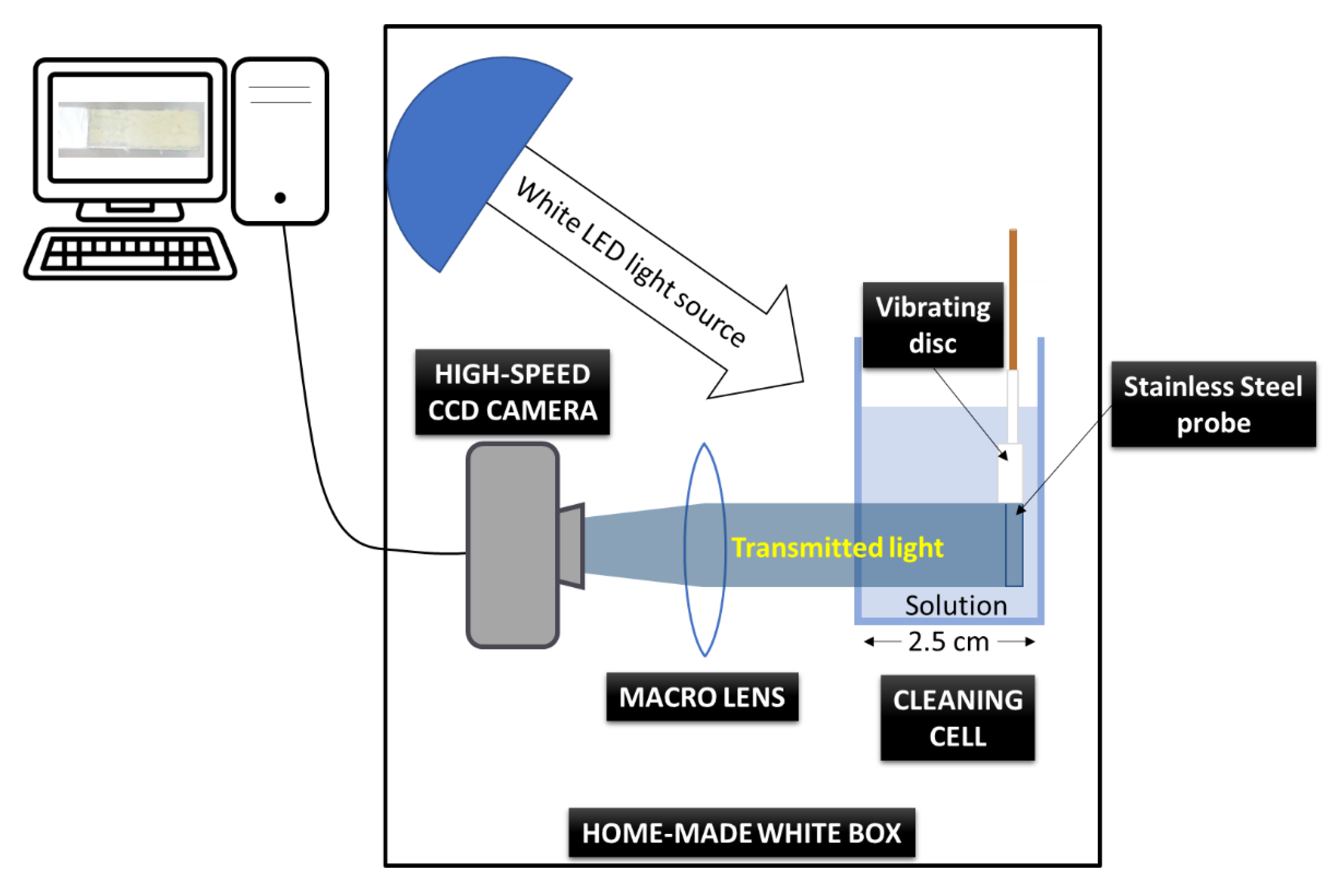
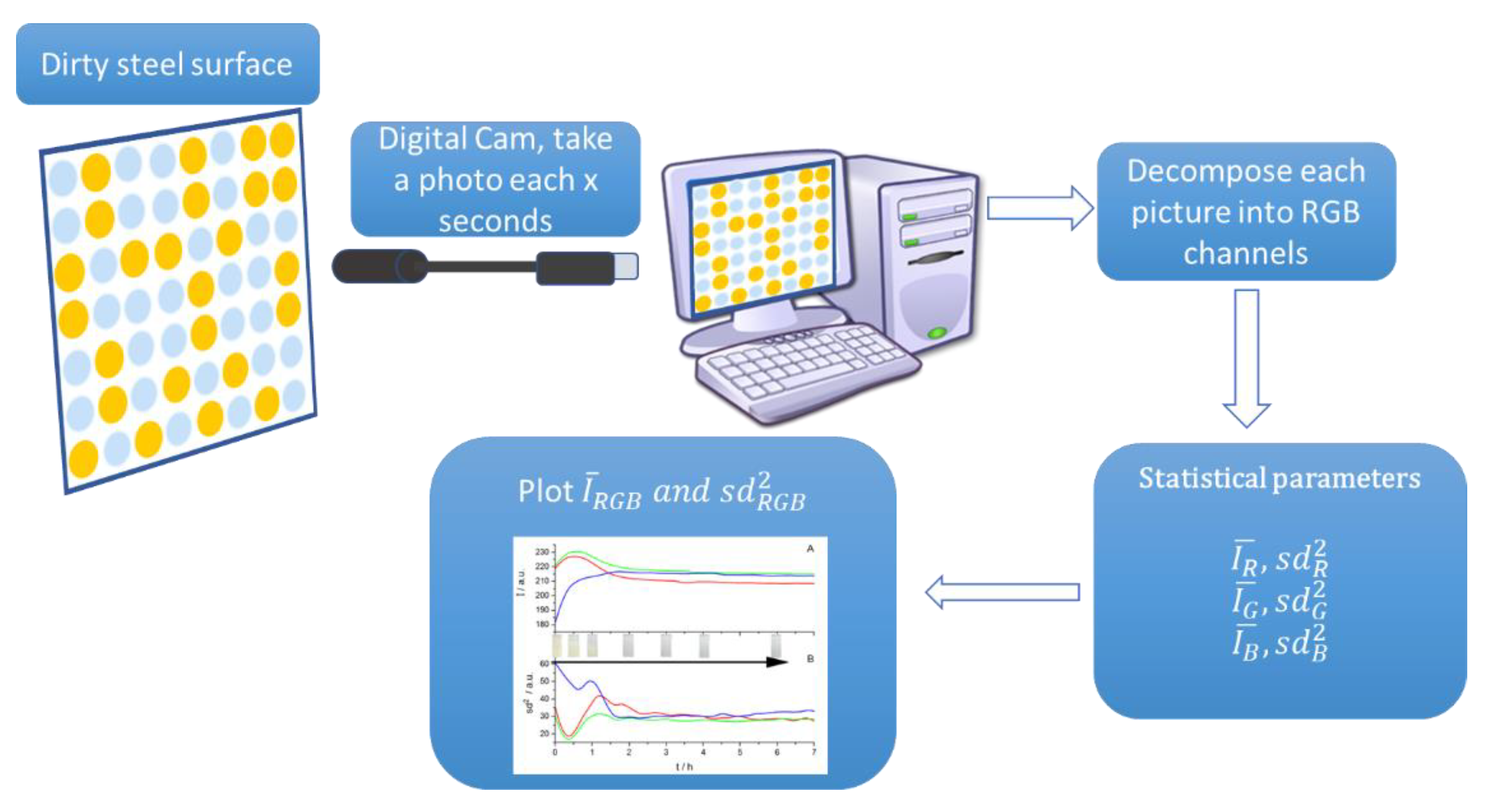
2. Materials and Methods

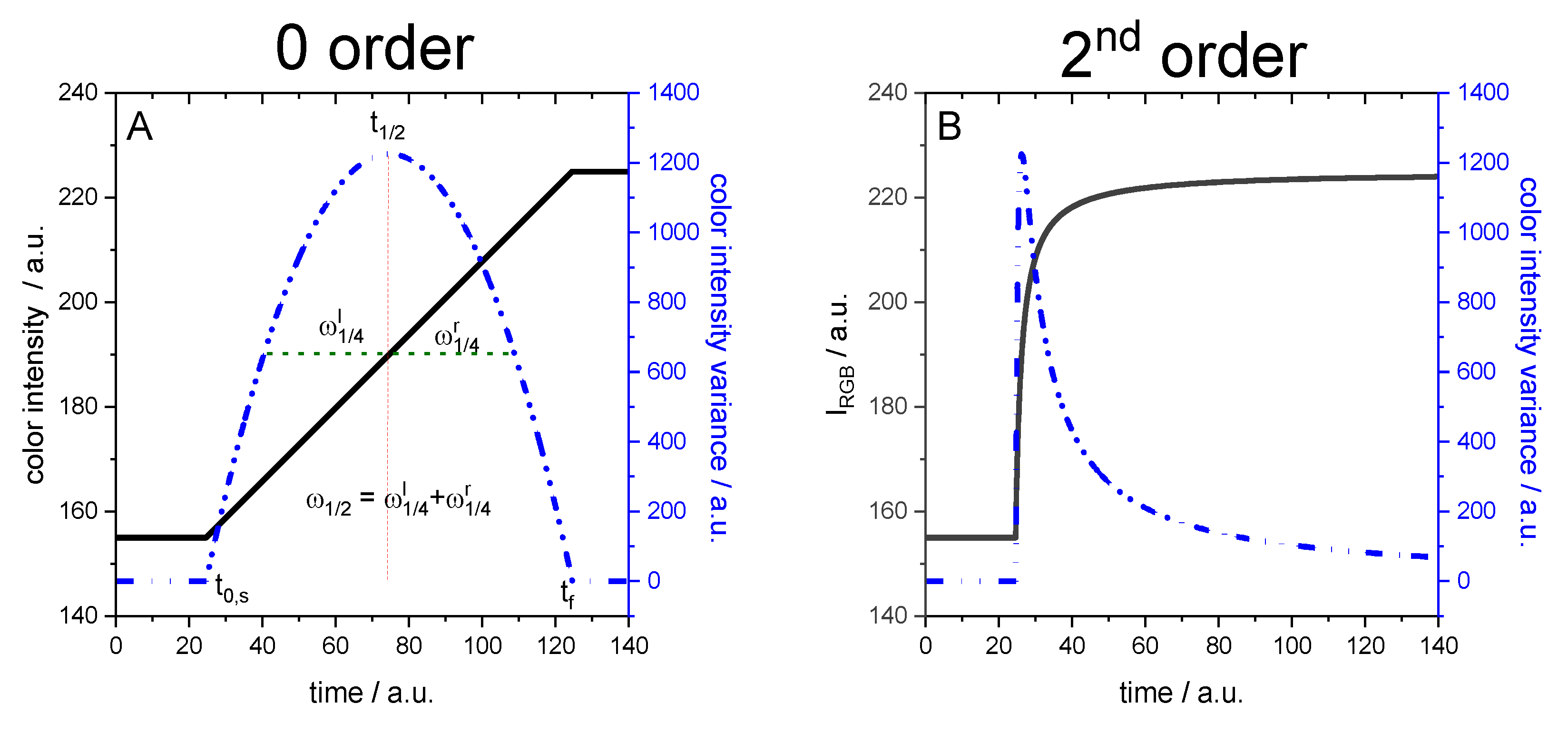
Metal samples consisted of a commercial stainless steel 316 pipeline and stainless steel 316 coupons of 6 × 1 cm, where an area of 2 × 1 cm was covered with peanut butter and the rest of the probe was covered with isolating Teflon tape.

The peanut butter was a commercial brand (Lucky Joe) and its composition, based on nutritional information provided in the label, is shown in

Table 1. Peanut butter: summary nutritional information.

Nutritional Information	Per 100 g
Fats	51 g
Saturated fats	11 g
Carbohydrates	15 g
Sugars	8 g
Proteins	25 g
Salt (NaCl)	1.1 g

.

The cleaning products were provided by Christeyns. Two commercial detergents were used for this study. For the dissolution test of fatty residues such as peanut butter, MIDA FOAM 174 UW (MF174UW) was used. This product is a liquid foaming detergent with low alkalinity and great degreasing power. Its composition, based on non-ionic surfactants, organic solvents and sequestrants, allows great cleaning power against organic residues and grease and mineral oils in food and beverage production environments. On the other hand, for the removal of the black residue, BETELENE MS-NP (BMSNP) was used. It is an acid descaling detergent based on methanesulfonic acid as the active ingredient. Methanesulfonic acid is a sustainable alternative to conventional acids used in detergents. These detergents contain a mixture of surfactants, sequestering agents, solvents and specific acidic or alkaline raw materials for the complete removal of the protein, fat and carbohydrate content of the chosen residue. The safety data sheet and technical information for each tested product describe its main properties and characteristics [51]. These products were used in dilutions of 5% BMSNP and 1% or 3% for MF174UW. The water for these dilutions was ultrapure water (18 MOhms cm). The mechanical action was simulated by applying a flat vibrator (DC3V 80 mA 11,000 rpm, 0.8 cm² surface area) to the steel sample immersed in a detergent solution. The temperatures at which the prepared dilutions were applied were 20 °C and 40 °C. Temperature was measured with a sensitivity of 0.1 °C and was controlled by means of a heating plate, obtaining a stable temperature with variations during the experiment of less than 0.5 °C.

The acquisition of digital images was carried out with the help of a digital camera (EPA-503278) with a resolution of 640 × 480 pixels and 24 bits of color deep in RGB space. Images were sequentially recorded at each time interval, adapting to the expected speed of the cleaning process (Figure 1). After the acquisition of the images and with the help of proprietary software, the mean color intensity for the RGB coordinates and their variance in the studied region of the surface was obtained for each one of the images (Figure 2).

Modelization

First, let us consider two simplified and ideal models by which the cleaning process can take place and the expected digital image results for each process. The purpose of this section is to gain a better understanding of the experimental results from real samples. In the first model, the cleaning took place by the chemical attack of the detergent product with the consequent complete dissolution of the deposited soiling, layer by layer. As the dissolution of the outermost layers of dirt exposed a new layer of dirt with the same surface color and homogeneity, but with a decreasing thickness, the cleaning process showed an apparent latency period without any color change, despite the dissolution process taking place. At a certain moment, the last layer of dirt began to disappear, exposing the bare metal surface. We can define this time as $\left(t_{0,s}\right)$, the first time at which the metal surface appears.

This process results in changes of color homogeneity and intensity of the image due to the emergence of new colored pixels. Depending on the color of the dirt layer and the bright metal surface, the change in mean color intensity can be either positive or negative. As the metal surface becomes more exposed and at least two different colored surfaces appear at the same time, the variance always increases initially. Variance reaches a maximum value, which is interpreted as the point where the color dispersion is maximum. In other words, this is the time at which half of the metal surface is covered by the layer of dirt and the other half is clean. We call this time the half-life time of surface cleaning process ($t_{1/2})$. It is important to note that this time is not the half-life time of the complete cleaning process since it depends on the thickness of the dirt layer. From this point on, the dirt layer will continue to dissolve, and the color of the metal surface will increasingly prevail, making the surface more homogeneous and thus decreasing the variance. In an ideal situation, at the end, the entire surface is clean and this will be identified by the fact that the average color intensity no longer changes, and the variance has returned to a minimum and constant value. This is the final time of the cleaning process ($t_f$).

Figure 3 shows two simulations of how these parameters (mean color intensity and color intensity variance) evolve over time for a cleaning process considering this dissolution mechanism and assuming that the analyzed region of the image of $n_p$ pixels changes its color between a color intensity $I_1$ characteristic of the dirt layer to a final color intensity $I_2$, characteristic of the clean metal surface. We also suppose an irreversible process governed by a kinetic constant $k$. Mechanical action, such as stirring the dissolution, can speed up the process by removing the layers of solvent that are more concentrated in the dirt from the metal surface. The shape of these curves is characterized by the equations collected in

Table 2. Peak widths $\left({\mathrm{\omega }}_{1/2}\right)$ and half peak widths $\left({\mathrm{\omega }}_{1/4}\right)$ of variance versus time for different kinetic orders ($\alpha$ in Equation (3)). $n_p$ is the number of pixels in the image, $I_1$ is the mean color intensity characteristic of the dirt layer, $I_2$ is characteristic of the clean metal surface and $k$ is the kinetic constant of the irreversible process of cleaning [44].

Order	$\overline{\mathit{I}}$	$\mathit{s}{\mathit{d}}^2$	${\mathit{\omega }}_{1/2}$	${\mathit{\omega }}_{1/4}^{\mathit{r}}$	${\mathit{\omega }}_{1/4}^{\mathit{l}}$	$\frac{{\mathit{\omega }}_{1/4}^{\mathit{r}}}{{\mathit{\omega }}_{1/4}^{\mathit{l}}}$
0	$I_1+{\displaystyle \frac{I_2-I_1}{n_p}}{k}_{1}t$	${\displaystyle \frac{k{\left(I_2-I_1\right)}^2\left(n_p-kt\right)t}{n_p^2}}$	${\displaystyle \frac{n_p}{k\sqrt{2}}}$	${\displaystyle \frac{n_p}{k\sqrt{8}}}$	${\displaystyle \frac{n_p}{k\sqrt{8}}}$	1
1	$I_2+{\displaystyle \frac{\left(I_1-I_2\right)}{e^{kt}}}$	${\displaystyle \frac{\left(e^{kt}-1\right){\left(I_2-I_1\right)}^2}{e^{2kt}}}$	${\displaystyle \frac{1.76}{k}}$	${\displaystyle \frac{1.23}{k}}$	${\displaystyle \frac{0.53}{k}}$	2.3
2	${\displaystyle \frac{kt{\left(I_2-I_1\right)}^2{n}_p}{{\left(kt{n}_p+1\right)}^2}}$	${\displaystyle \frac{kt{\left(I_2-I_1\right)}^2{n}_p}{{\left(kt{n}_p+1\right)}^2}}$	${\displaystyle \frac{5.66}{k{n}_p}}$	${\displaystyle \frac{4.83}{k{n}_p}}$	${\displaystyle \frac{0.83}{k{n}_p}}$	5.8

$\left(\mathrm{r}\right)$ and (l) refers to the right part and the left part of the variance peak, respectively.

[44,46]. The mean color intensity ($\overline{I}$), the variance $s{d}^2$, the peak widths (${\omega }_{1/2}$), the peak half-widths (${\omega }_{1/4}$ left and right side) and the ratio between the peak half-widths of variance peaks depends on the kinetic orders (0,1,2) [41,44].

It should be noted that this last ratio can be interpreted as a measure of the symmetry of variance peaks.

Considering that the cleaning rate is directly related to the color change rate of the metal surface, we can propose a kinetic rate law for the cleaning process as follows:

$$cleaningrate=-{\displaystyle \frac{{\mathrm{d}\mathrm{n}}_{\mathrm{d}\mathrm{c}}}{dt}}=\mathrm{k}·{\mathrm{n}}_{\mathrm{d}\mathrm{c}}^{\alpha }$$

(3)

In Equation (3) $n_{dc}$ refers to the number of pixels with color of the dirt surface and $\alpha$ the kinetic order for the cleaning process. It should be noted that the mean color intensity $\overline{I}$ of the selected surface depends directly on the number of pixels with the dirt color, $n_{dc}$:

$$\overline{I}={\displaystyle \frac{{\mathrm{n}}_{\mathrm{d}\mathrm{c}}{I}_1+(n_p-n_{dc})I_2}{n_p}}=n_{dc}{\displaystyle \frac{\left(I_1-I_2\right)}{n_p}}+I_2$$

(4)

where $I_1$ corresponds to the characteristic color of the dirt surface and $I_2$ the characteristic color of the clean surface.

In accordance with Table 2, these peaks will show a symmetrical shape only for kinetics of order 0 ($\alpha =0)$, while for kinetics of higher orders, the right side of the peak appears wider than the left side [41,44].

In the second proposed mechanism, the cleaning product chemically attacks the layer of dirt, changing both the mechanical properties and the adhesion to the metal surface. The layer of dirt will eventually become easier to peel off from the metal surface and easier to break off. Therefore, this proposed mechanism necessarily adds to the chemical cleaning some mechanical actions when dirt is removed in portions.

This second proposed mechanism also starts with a chemical attack on the surface of the deposited dirt layer that does not necessarily involve the dissolution of the dirt layer. In some cases, the chemical attack will involve a change in the physical–chemical properties of the layer of dirt which can be observed as a color change of the layer of dirt. Therefore, we would observe changes in color intensity from the original color to the color of the coating after the chemical attack and a peak in the evolution over time of the variance [44] similar to that simulated in Figure 3.

Once the chemical attack has occurred, the mechanical action removes this layer of dirt from the surface of the metal, and both the mean color intensity and the variance will show irregular evolutions until the clean metal surface appears. These irregularities can be masked if the surface area studied is large enough and the pieces of dirt leaving the surface are not very large in size. Note that this process and its speed will be totally dependent on the type of mechanical action and its extent. As the layer of dirt is not dissolved, portions of dirt pass to the solution as a suspension or precipitate, depending on the relative density of the dirt. In the case of no mechanical action being applied in this type of cleaning mechanism, the removal of the layer of dirt from the metal surface may not occur and it may remain weakly adhered to the metal probe.

3. Results and Discussion

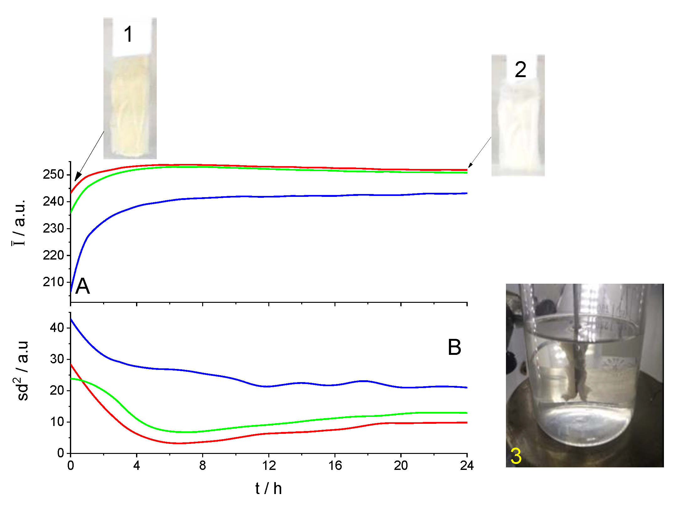
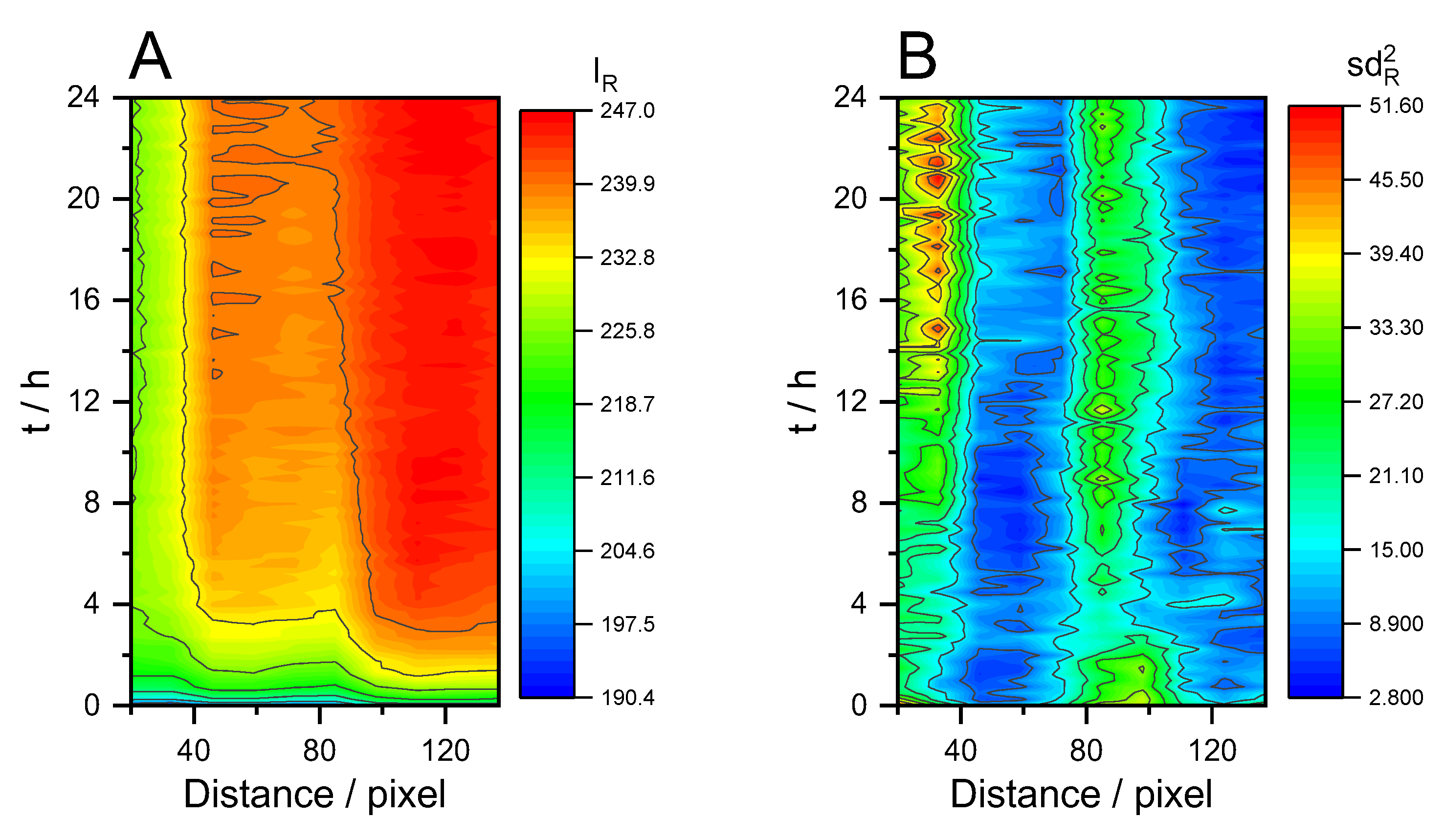
3.1. Cleaning by Dissolution

In the first case, a piece of industrial pipe with a blackish layer of dirt, caused by its normal use and of unknown composition, was cleaned by immersion in an aqueous solution of BMSNP (5%) whose active ingredient was a methanesulfonic acid solution. This cleaning process occurs without mechanical stirring over 24 h. An accelerated video of this cleaning process can be seen in Video S1 (Supplementary Materials).

The time evolution of mean color intensity for the three colors and the corresponding color intensity variance of the whole pipe surface is depicted in Figure 4. During the first two hours, a small increase in the color intensities was observed (Figure 4A). This may have been due to the beginning of the chemical attack of the cleaning product on the stain, or to a simple hydration of the outermost layer. The first significant color changes on the surface were observed at times between 8 and 12 h, when the surface of the uncoated metal began to appear ($t_{0,s}$). These color changes continued until 18 h ($t_f$), when it was observed that the color intensities hardly changed with time, which corresponded to the surface of the metal being now clean. Regarding the time evolution of variance, a peak appeared at about 15.5 h which corresponded to the time where one half of the analyzed pipe surface remained black, and the other half showed the final white-gray color ($t_{1/2},$ Figure 4B). Before this peak, a shoulder at about 9 h was observed. This behavior can be explained by the fact that the analyzed surface was large enough and the dirt layer proved not homogeneous in thickness or chemical composition (see EDX microanalysis data in Figure S1, Supplementary Materials). The inhomogeneity of the dirt layer can mean that it takes longer for regions with a thicker layer to have all of the dirt removed. Translating this into a change in variance, there will be a portion of the surface where 50% of the last layer has been removed and therefore the variance will be at its maximum, while other portions have not yet reached 50% and will have lower values. This means that the ideal predicted peak shape is partially deformed, and shoulders can be observed on the peak. When a small region is analyzed, the peak shape appears without a shoulder.

One of the advantages of digital video analysis is the simultaneous spatiotemporal study of different areas of the test probe. Due to the non-homogeneity of the dirt on the pipe surface, we proceeded to study the evolution of these kinetic parameters in two regions of the sample marked as ‘upper left’ and ‘lower right’ in Figure 5. Compared with data in Figure 4, we observed that the cleaning of the last layer of dirt started around 12 h ($t_{0,s}$) on the left side of the sample. After that, we observed that the maximum and constant color intensity of the left side was reached at about 16 h, over a relatively shorter time than was the case for the entire surface. Something similar was observed for the evolution of the variance with time. In this last case, the shape of the variance peak looked more symmetrical than the peaks obtained from the right side or for the whole metal surface analyzed. This result can be explained by a more homogeneous region analyzed on the left side of the sample. Also, the peak for the maximum occurred at 14.5 h, 1 h before the maximum for the whole surface analysis. Looking now at the right side of the sample, a steep decrease of color intensities was observed between 7 h and 12 h. This means that the surface was becoming darker. A possible explanation is that the first hydrated layer had been removed and the innermost layer of dirt was visible. After 12 h, the color intensity increased for the three coordinates until it reached a maximum and constant value at about 18 h. Changes were not significant once the surface was clean. For the time evolution of the variance, minimal changes occurred before 12 h, then an increase to define a peak with a maximum value just before 16 h, followed by a sharp decrease and from 18 h onwards hardly any change.

Table 3. Characteristic times for the cleaning of a piece of pipe with a methanesulfonic acid-based product, BMSNP (5%), focusing on different parts of the sample extracted from Figure 4 and Figure 5.

Region	${\mathit{t}}_0$/h	${\mathit{t}}_{1/2}$/h	${\mathit{t}}_{\mathit{f}}$/h	${\mathit{\omega }}_{1/4}^{\mathit{l}}$/h	${\mathit{\omega }}_{1/4}^{\mathit{r}}$/h	${\mathit{\omega }}_{1/4}^{\mathit{r}}/{\mathit{\omega }}_{1/4}^{\mathit{l}}$
Upper left	12.4	14.2	16	0.9	0.8	0.95
Lower right	12.5	15.4	16.5	1.3	1.2	0.92
Global	11.5	15.6	18.7	2.5	1.7	0.70

collects characteristic times and peak half-widths of variance for the three regions analyzed. First, characteristic times are lower in the left region than in the right region or the global measurement. In particular, the half-life time appears 1.2 h earlier in the left region. A second observation involves the peak width and half-widths. For the left region, significantly lower values are observed, confirming that the analyzed region was more homogeneous than in the other two cases. Finally, the ratio of the peak half-widths is close to unity in all three cases, somewhat smaller for the study of the entire surface. According to previously published models, these values near the unity can be interpreted as an order 0 kinetics for this cleaning process.

To observe these differences in better detail, a 3D map of color variation versus time and distance from the left end of the sample is presented [43]. As a representative result, Figure 6 shows the 3D map of mean color intensity and variance of red color. Several observations can be drawn from Figure 6. On the one hand, for longer times, the color of the surface is not homogeneous with a lower color intensity being observed in the central part, which means that it is somewhat more blackened than the ends. On the other hand, the isochromatic lines are not horizontal, but follow an inverted U-shape, indicating that the central part changes its color later than the periphery. Another interesting observation is that the isochromatic lines are closer together in the central region of the metal than in the outer regions. This distance between isochromatic lines is directly related to the rate of color change. Therefore, once the last layer has begun to disappear in the central region, the dissolution rate appears to be somewhat faster than the dissolution rate in the outer zones. If we analyze the 3D plot of the evolution of the color variance against the elapsed time and the distance to the left boundary of the sample, we can remark on some points. First, changes in variance do not occur gradually. They occur when the last layer of dirt is dissolved and the color of the metal is observed. As predicted by the theoretical models for the evolution of the variance over time, it is observed that the variance initially increases when the dissolution of the last layer begins, reaches the maximum value, and finally decreases as the observed surface becomes more homogeneous again. This maximum corresponds to the characteristic half-life time $t_{1/2}$ previously defined. Note that this time is not the same for every position on the sample. It shows higher values in the central region and lower values on the outer sides. Note also how at this point, the central region shows higher variance values for times longer than 18 h than the variance at the outer sides. This is because there are remains of the dirt layer after 24 h in the central region, while the outer sides appear cleaner. Other interesting observations are that variance changes begin at shorter times at the outer sides, and the homogeneous color is also reached earlier in these regions.

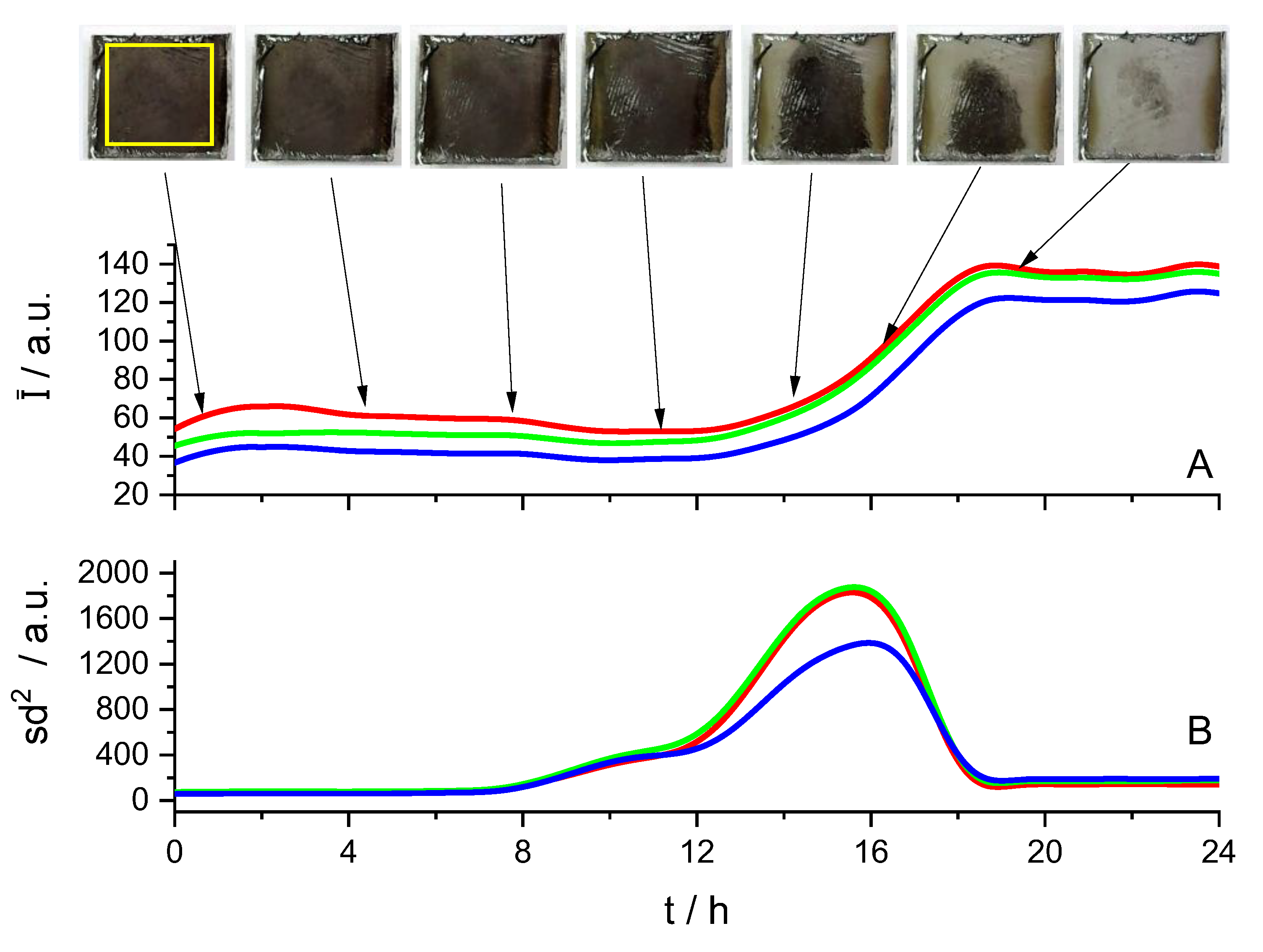
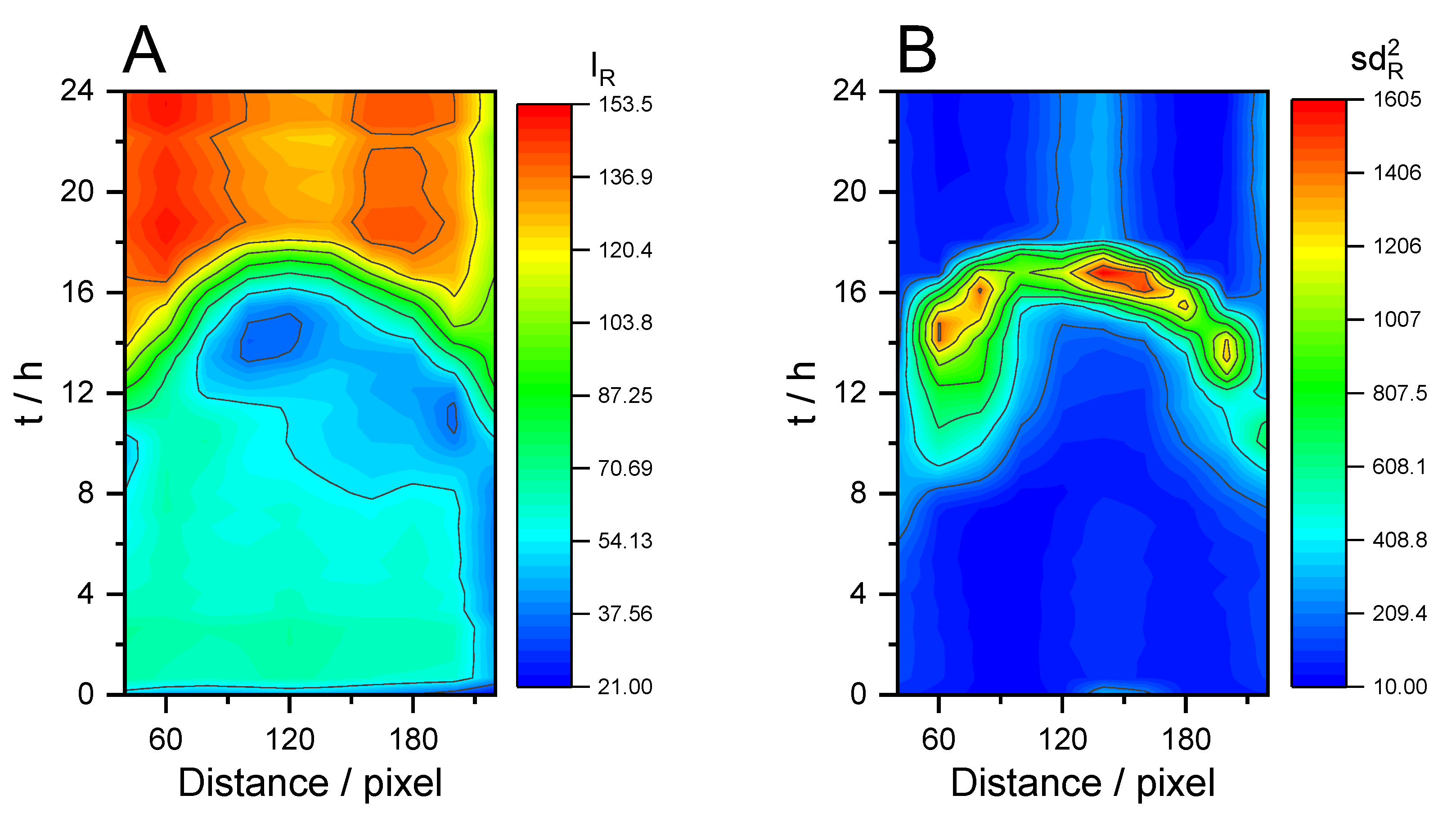
3.2. Peeling off Cleaning

In the second case, chemical attack on the layer of dirt was combined with mechanical action. For this purpose, we studied the cleaning of steel plates on which 0.28 g of peanut butter had been previously spread. The steel plate was submitted to the action of a flat vibrator at 11,000 rpm during the cleaning process.

To study the effect of the cleaning product on the peanut butter residue, this cleaning process was followed by the acquisition of sequential images during the necessary time until the entire surface was cleaned. The original mean color of the peanut butter in our lighting conditions was ocher (230,222,193) (image 1 in Figure 7), changing after a short time and after the chemical attack to a quite intense white color (250,250,240) (image 2 in Figure 7). Therefore, color increments of (20,28,47) units for each color coordinate were observed. This made the changes more evident in the blue coordinate than in red or green, although they were also noteworthy for these coordinates. After the test was completed, when the steel plate was removed from the cleaning solution, it was observed that the peanut butter layer had a gelatinous appearance, its volume had increased considerably, the color was much whiter and it easily peeled off the surface in the form of a film (image 3 in Figure 7). An accelerated video of this process can be seen in the Supplementary Materials (Video S2).

Figure 7 shows how the chemical attack of the cleaning product MF174UW took place during the first 4–6 h until the mean color intensity (Figure 7A) and its variance (Figure 7B) reached almost constant values for the three colors. Unexpectedly, the variance did not show a peak as in theory (Figure 3) for the change from the ochre color (image 1 in Figure 7A) to white (image 2 in Figure 7A). We can explain this fact considering that the initial color dispersion for the steel surface coated with peanut butter was high enough due to the spreading procedure of peanut butter, which caused a non-homogeneous layer, and because some shadows were formed in our lighting conditions. Therefore, we observed only a decrease from the inhomogeneous color of the peanut butter to the more homogeneous color of the chemically attacked layer. On the other hand, the 3D plots of mean red color intensity and its variance against the elapsed time and the distance in pixels from the top of the metal sample (Figure 8) showed that the color changes occurred earlier and more extensively on the bottom of the metal plate. However, the swelling of the peanut butter might have affected the quality and accuracy of these observations (image 3 in Figure 7).

In the following experiment, we added the effect of mechanical action generated by a flat vibrating motor at 11,000 rpm during the chemical peanut butter cleaning. In Supplementary Materials there is an accelerated video corresponding to this experiment. For the same composition (1% MF174UW), the chemical attack of the cleaning product was also observed since there was a color change from ocher to white (Figure 9). After the chemical attack, some fragments peeled off from the peanut butter. In terms of color change, the blue color hardly changed in this last step, but the intensity of red and green decreased as the surface of the steel became darker (Figure 9A).

The variance evolution of the three colors over time (Figure 9B) showed the effect of chemical attack during the first 30 min, as before, due to the bleaching of peanut butter. Then, a peak appeared in the three coordinates, but not synchronously. The maximum for blue appeared earlier than for the other two colors, caused by the change from ocher to white, which involved the greatest increase in the blue coordinate (Figure 9A). Thus, red and green variance peaks proved more appropriate to study the cleaning process since in this case, changes of variance were mainly due to changes from the white chemically attacked peanut butter to the white-gray of the bare steel surface. The peak observed for green and red color around 75 min corresponds to the time when one half of the surface remained covered by peanut butter and the other half was uncovered. Careful observation of the shape of the red color variance shows that it was quite asymmetrical, as corresponded to first or second kinetic orders (see Figure 3). Due to overlapping of two processes (chemical attack and peeling off), the resulting shape of these curves did not allow an accurate estimation of the half width at half maximum to discern between first and second kinetic orders (Table 2), but we can discard a zero-order kinetics reaction. An accelerated video of this process can be seen in the Supplementary Materials (Video S3).

At higher concentration of the cleaning agent (3% of MF174UW), we expected an acceleration of the cleaning process. Initially, the first color change to white was not observed. If we assume that the chemical attack was faster, then it is possible that the breakage and loss of adhesion to the metal may have taken place before the color change. Three-dimensional plots of blue color intensity and their variance against the elapsed time and the distance from the top of the electrode are presented in Figure 10. For the blue color intensity, we see that the final color was reached before 30 min (Figure 10A). The maximum of variance was reached at about 15 min without many differences from the distance from the top of the electrode (Figure 10B). The observed color changes were smoothed by the mechanical effect of the vibration together with the higher concentration of the detergent.

Table 4. Characteristic times for the process of cleaning peanut butter from steel with the product MF174UW in concentrations of 1% and 3%, at a temperature of 20 °C and 40 °C, and without mechanical action and with mechanical action (vibration). Gray shaded cells indicate that this process was not observed.

Conditions for the Cleaning Process			1st Process (Whitening)			2nd Process (Peeling off)
T/K	Vibration	Conc. (%)	${\mathit{t}}_0$/s	${\mathit{t}}_{1/2}$/s	${\mathit{t}}_{\mathit{e}\mathit{n}\mathit{d}}$/s	${\mathit{t}}_0$/s	${\mathit{t}}_{1/2}$/s	${\mathit{t}}_{\mathit{e}\mathit{n}\mathit{d}}$/s
293	NO	1%	160		2255
293	NO	3%	20		1280
293	YES	1%				810	1240	2030
293	YES	3%				0	500	1270
313	NO	1%	0		4000
313	NO	3%				902	2058	2556
313	YES	1%				460	750	1040
313	YES	3%				0	177	414

summarizes the results of the cleaning process at two temperatures, for two concentrations of the cleaning product and applying, or not, vibration as a mechanical action that helped the cleaning of the product. Table 4 allows us to corroborate that increasing the concentration of the cleaning product from 1% to 3% multiplied the cleaning speed by approximately two. It can be assumed that under the experimental conditions of this work, with the use of the vibrating electrode, it was possible to renew the solution in the vicinity of the peanut butter layer continuously. Therefore, the MF174UW concentration remained constant. If we consider a simplified model in which the cleaning rate depends on both, the surface concentration of dirt (${\mathsf{\Gamma }}_d)$ and on the solution concentration of MF174UW ([MF174UW]), we can write a rate equation as:

$$rate=k{\mathsf{\Gamma }}_{\mathrm{d}}^{\alpha }{\left[MF174UW\right]}^{\beta }=k_{ap}{\mathsf{\Gamma }}_{\mathrm{d}}^{\alpha }$$

(5)

$$k_{ap}=k{\left[MF174UW\right]}^{\beta }$$

(6)

Therefore, if the concentration is multiplied by 3 and the speed (estimated from $t_{end}$ in Table 4) by (1.6–2.5), this means an experimental apparent kinetic order $\beta$ for MF174UW of 0.4–0.8.

We can also estimate the temperature effect on the cleaning rate as an increase from 20 °C to 40 °C reduces the cleaning times by approximately 2–3 times, and this allows us to estimate the apparent activation energy of the cleaning process, assuming an Arrhenius dependence of kinetics constant on the temperature (about 25–40 kJ mol⁻¹).

4. Conclusions

Monitoring of color changes during the cleaning process of a metal surface by digital images allowed not only qualitative but also quantitative evaluation of the homogeneity and kinetics of the cleaning process. The use of spatiotemporal data analysis for this purpose has a great advantage over other forms of online monitoring of the cleaning process because it allowed the homogeneity of the entire surface and the final quality of the process to be evaluated.

The characteristic times defined from the curves of color intensities and variance evolution versus time were excellent indicators not only of the rate of the process, but also of the final homogeneity of the cleaning process. The analysis of these parameters showed how the kinetics of the cleaning process were quantitatively affected by the concentration of the cleaning product, the temperature and the mechanical action exerted, even estimating an activation energy for the cleaning process. Finally, this type of analysis allowed us to obtain an initial estimation of the kinetics of the cleaning process, which were used to estimate the time needed to finish the cleaning process and, based on this, to optimize the experimental conditions.

References

1. Pontefract, R. Bacterial Adherence—Its Consequences in Food-Processing. Can. Inst. Food Sci. Technol. J. 1991, 24, 113–117. [Google Scholar] [CrossRef]
2. Boulané-Petermann, L. Processes of Bioadhesion on Stainless Steel Surfaces and Cleanability: A Review with Special Reference to the Food Industry. Biofouling 1996, 10, 275–300. [Google Scholar] [CrossRef] [PubMed]
3. Jackson, L.S.; Al-Taher, F.M.; Moorman, M.; DeVries, J.W.; Tippett, R.; Swanson, K.M.J.; Fu, T.-J.; Salter, R.; Dunaif, G.; Estes, S.; et al. Cleaning and Other Control and Validation Strategies to Prevent Allergen Cross-Contact in Food-Processing Operations. J. Food Prot. 2008, 71, 445–458. [Google Scholar] [CrossRef]
4. Rossi, S.; Leso, S.M.; Calovi, M. Study of the Corrosion Behavior of Stainless Steel in Food Industry. Materials 2024, 17, 1617. [Google Scholar] [CrossRef]
5. Chung, M.M.S.; Tsai, J.-H.; Lu, J.; Padilla Chevez, M.; Huang, J.-Y. Microbubble-Assisted Cleaning To Enhance the Removal of Milk Deposits from the Heat Transfer Surface. ACS Sustain. Chem. Eng. 2022, 10, 8380–8387. [Google Scholar] [CrossRef]
6. Dallagi, H.; Jha, P.K.; Faille, C.; Le-Bail, A.; Rawson, A.; Benezech, T. Removal of Biocontamination in the Food Industry Using Physical Methods: An Overview. Food Control 2023, 148, 109645. [Google Scholar] [CrossRef]
7. Elsayed, S.; Galal, H.; Allam, A.; Schmidhalter, U. Passive Reflectance Sensing and Digital Image Analysis for Assessing Quality Parameters of Mango Fruits. Sci. Hortic. 2016, 212, 136–147. [Google Scholar]
8. Alonso, V.P.P.; Lemos, J.G.; Nascimento, M.d.S.d. Yeast Biofilms on Abiotic Surfaces: Adhesion Factors and Control Methods. Int. J. Food Microbiol. 2023, 400, 110265. [Google Scholar] [CrossRef]
9. Crandall, P.G.; O’Bryan, C.A.; Wang, D.; Gibson, K.E.; Obe, T. Environmental Monitoring in Food Manufacturing: Current Perspectives and Emerging Frontiers. Food Control 2024, 159, 110269. [Google Scholar] [CrossRef]
10. Gomes, L.C.; Saubade, F.; Amin, M.; Spall, J.; Liauw, C.M.; Mergulhão, F.; Whitehead, K.A. A Comparison of Vegetable Leaves and Replicated Biomimetic Surfaces on the Binding of Escherichia coli and Listeria monocytogenes. Food Bioprod. Process. 2023, 137, 99–112. [Google Scholar] [CrossRef]
11. Wan Omar, W.H.; Mahyudin, N.A.; Azmi, N.N.; Mahmud Ab Rashid, N.-K.; Ismail, R.; Mohd Yusoff, M.H.Y.; Khairil Mokhtar, N.F.; Sharples, G.J. Effect of Natural Antibacterial Clays against Single Biofilm Formation by Staphylococcus Aureus and Salmonella Typhimurium Bacteria on a Stainless-Steel Surface. Int. J. Food Microbiol. 2023, 394, 110184. [Google Scholar] [CrossRef] [PubMed]
12. Chmielewski, R.A.N.; Frank, J.F. Biofilm Formation and Control in Food Processing Facilities. Compr. Rev. Food Sci. Food Saf. 2003, 2, 22–32. [Google Scholar] [CrossRef] [PubMed]
13. Orihuel Iranzo, E.; Bertó Navarro, R.; Lorenzo Cartón, F.; López Tormo, C.; San José Serran, C.; Orgaz Martín, B. Biofilm-Marking Composition and Method for Detection of Same on Surfaces. European Patent EP2634260A1, 4 November 2013. [Google Scholar]
14. Cappitelli, F.; Polo, A.; Villa, F. Biofilm Formation in Food Processing Environments Is Still Poorly Understood and Controlled. Food Eng. Rev. 2014, 6, 29–42. [Google Scholar] [CrossRef]
15. Galié, S.; García-Gutiérrez, C.; Miguélez, E.M.; Villar, C.J.; Lombó, F. Biofilms in the Food Industry: Health Aspects and Control Methods. Front. Microbiol. 2018, 9, 898. [Google Scholar] [CrossRef]
16. Kabwanga, I.T.; Yetişemiyen, A.; Nankya, S. Dairy Industrial Hygiene: A Review on Biofilms Challenges and Control. Int. J. Res. Granthaalayah 2018, 6, 268–273. [Google Scholar] [CrossRef]
17. Puga, C.H.; Dahdouh, E.; SanJose, C.; Orgaz, B. Listeria Monocytogenes Colonizes Pseudomonas Fluorescens Biofilms and Induces Matrix Over-Production. Front. Microbiol. 2018, 9, 1706. [Google Scholar] [CrossRef]
18. Lorenzo, F.; Sanz-Puig, M.; Bertó, R.; Orihuel, E. Assessment of Performance of Two Rapid Methods for On-Site Control of Microbial and Biofilm Contamination. Appl. Sci. 2020, 10, 744. [Google Scholar] [CrossRef]
19. Brozkova, I.; Cervenka, L.; Motkova, P.; Fruhbauerova, M.; Metelka, R.; Svancara, I.; Sys, M. Electrochemical Control of Biofilm Formation and Approaches to Biofilm Removal. Appl. Sci.-Basel 2022, 12, 6320. [Google Scholar] [CrossRef]
20. Sha, J.; Xu, C.; Xu, K. Progress of Research on the Application of Nanoelectronic Smelling in the Field of Food. Micromachines 2022, 13, 789. [Google Scholar] [CrossRef]
21. Zhang, X.; Yang, C.; Yang, K. Novel Antibacterial Metals as Food Contact Materials: A Review. Materials 2023, 16, 3029. [Google Scholar] [CrossRef]
22. de Larios, J.M.; Zhang, J.; Zhao, E.; Gockel, T.; Ravkin, M. Evaluating Chemical Mechanical Cleaning Technology for Post-CMP Applications. Micro 1997, 15, 61. [Google Scholar]
23. Toure, Y.; Mabon, N.; Sindic, M. Soil Model Systems Used to Assess Fouling, Soil Adherence and Surface Cleanability in the Laboratory: A Review. Biotechnol. Agron. Société Environ. 2013, 17, 527–539. [Google Scholar]
24. Chen, Y.L.; Zhu, S.M.; Lee, S.J.; Wang, J.C. The Technology Combined Electrochemical Mechanical Polishing. J. Mater. Process. Technol. 2003, 140, 203–205. [Google Scholar] [CrossRef]
25. Memisi, N.; Moracanin, S.V.; Milijasevic, M.; Babic, J.; Djukic, D. CIP Cleaning Processes in the Dairy Industry. Procedia Food Sci. 2015, 5, 184–186. [Google Scholar] [CrossRef]
26. Fryer, P.J.; Christian, G.K.; Liu, W. How Hygiene Happens: Physics and Chemistry of Cleaning. Int. J. Dairy Technol. 2006, 59, 76–84. [Google Scholar] [CrossRef]
27. Orihuel, E.; Bertó, R.; Lorenzo, F.; López, C. Mechanical Energy Balance in Surface Cleaning by Pressurised Water Spray: A Simplified Model. Ehedg Yearb. 2017, 2018, 32–37. [Google Scholar]
28. Padmanabhan, N.T.; John, H. Titanium Dioxide Based Self-Cleaning Smart Surfaces: A Short Review. J. Environ. Chem. Eng. 2020, 8, 104211. [Google Scholar] [CrossRef]
29. Leclercq-Perlat, M.-N.; Lalande, M. Cleanability in Relation to Surface Chemical Composition and Surface Finishing of Some Materials Commonly Used in Food Industries. J. Food Eng. 1994, 23, 501–517. [Google Scholar] [CrossRef]
30. Köhler, H.; Stoye, H.; Mauermann, M.; Weyrauch, T.; Majschak, J.-P. How to Assess Cleaning? Evaluating the Cleaning Performance of Moving Impinging Jets. Food Bioprod. Process. 2015, 93, 327–332. [Google Scholar] [CrossRef]
31. Lang, M.P.; Kocaoglu-Vurma, N.A.; Harper, W.J.; Rodriguez-Saona, L.E. Multicomponent Cleaning Verification of Stainless Steel Surfaces for the Removal of Dairy Residues Using Infrared Microspectroscopy. J. Food Sci. 2011, 76, C303–C308. [Google Scholar] [CrossRef]
32. Schöler, M.; Fuchs, T.; Helbig, M.; Augustin, W.; Scholl, S.; Majschak, J.-P. Monitoring of the Local Cleaning Efficiency of Pulsed Flow Cleaning Procedures. In Proceedings of the International Conference on Heat Exchanger Fouling and Cleaning, Schladming, Austria, 14–19 June 2009. [Google Scholar]
33. Detry, J.G.; Deroanne, C.; Sindic, M. Hydrodynamic Systems for Assessing Surface Fouling, Soil Adherence and Cleaning in Laboratory Installations. Biotechnol. Agron. Soc. Environ. 2009, 13, 427–439. [Google Scholar]
34. Davidson, C.A.; Griffith, C.J.; Peters, A.C.; Fielding, L.M. Evaluation of Two Methods for Monitoring Surface Cleanliness—ATP Bioluminescence and Traditional Hygiene Swabbing. Luminescence 1999, 14, 33–38. [Google Scholar] [CrossRef]
35. Rizzotto, F.; Khalife, M.; Hou, Y.; Chaix, C.; Lagarde, F.; Scaramozzino, N.; Vidic, J. Recent Advances in Electrochemical Biosensors for Food Control. Micromachines 2023, 14, 1412. [Google Scholar] [CrossRef] [PubMed]
36. Yang, S.; Gao, S.; Zhuang, Y.; Hu, W.; Zhao, J.; Yi, Z. Non-Destructive Sensor for Glucose Solution Concentration Detection Using Electromagnetic Technology. Micromachines 2024, 15, 758. [Google Scholar] [CrossRef]
37. Assaifan, A.K. Thiol-SAM Concentration Effect on the Performance of Interdigitated Electrode-Based Redox-Free Biosensors. Micromachines 2024, 15, 1254. [Google Scholar] [CrossRef] [PubMed]
38. de Oliveira Krambeck Franco, M.; Suarez, W.T.; Santos, V.B. dos Digital Image Method Smartphone-Based for Furfural Determination in Sugarcane Spirits. Food Anal. Methods 2017, 10, 508–515. [Google Scholar] [CrossRef]
39. Agrisuelas, J.; García-Jareño, J.J.; Perianes, E.; Vicente, F. Use of RGB Digital Video Analysis to Study Electrochemical Processes Involving Color Changes. Electrochem. Commun. 2017, 78, 38–42. [Google Scholar] [CrossRef]
40. Minz, P.S.; Sawhney, I.K.; Saini, C.S. Algorithm for Processing High Definition Images for Food Colourimetry. Measurement 2020, 158, 107670. [Google Scholar] [CrossRef]
41. Agrisuelas, J.; García-Jareño, J.J.; Vicente, F. Quantification of Electrochromic Kinetics by Analysis of RGB Digital Video Images. Electrochem. Commun. 2018, 93, 86–90. [Google Scholar] [CrossRef]
42. Kanchi, S.; Sabela, M.I.; Mdluli, P.S.; Inamuddin; Bisetty, K. Smartphone Based Bioanalytical and Diagnosis Applications: A Review. Biosens. Bioelectron. 2018, 102, 136–149. [Google Scholar] [CrossRef]
43. Agrisuelas, J.; García-Jareño, J.J.; Guillén, E.; Vicente, F. RGB Video Electrochemistry of Copper Electrodeposition/Electrodissolution in Acid Media on a Ternary Graphite:Copper:Polypropylene Composite Electrode. Electrochim. Acta 2019, 305, 72–80. [Google Scholar] [CrossRef]
44. Agrisuelas, J.; García-Jareño, J.J.; Guillén, E.; Vicente, F. Kinetics of Surface Chemical Reactions from a Digital Video. J. Phys. Chem. C 2020, 124, 2050–2059. [Google Scholar] [CrossRef]
45. Fan, Y.; Li, J.; Guo, Y.; Xie, L.; Zhang, G. Digital Image Colorimetry on Smartphone for Chemical Analysis: A Review. Measurement 2021, 171, 108829. [Google Scholar] [CrossRef]
46. Agrisuelas, J.; García-Jareño, J.J.; Vicente, F. A Statistical Interpretation of the Voltammetry of Adsorbed Substances under the Perspective View of the Digital Video Electrochemistry. Microchem. J. 2022, 181, 107844. [Google Scholar] [CrossRef]
47. Cánovas-Saura, A.; Serrano-Luján, L.; Beltrán, V.; Padilla, J. Neural Network-Based Digital Camera Spectrophotometer: Application to Chromogenic Technologies Characterization. ACS Appl. Opt. Mater. 2024, 2, 1403–1412. [Google Scholar] [CrossRef]
48. García-Jareño, J.J.; Agrisuelas, J.; Vargas, Z.; Vicente, F. Electrogeneration and Characterization of Poly(Methylene Blue) Thin Films on Stainless Steel 316 Electrodes—Effect of pH. Molecules 2024, 29, 3752. [Google Scholar] [CrossRef]
49. García-Jareño, J.J.; Agrisuelas, J.; Vicente, F. Overview and Recent Advances in Hyphenated Electrochemical Techniques for the Characterization of Electroactive Materials. Materials 2023, 16, 4226. [Google Scholar] [CrossRef]
50. Agrisuelas, J.; García-Jareño, J.J.; Piedras, M.; Vicente, F. Quality and Efficiency Control of Electrodeposition and Electrodissolution of Ni on a Ternary Composite Electrode Followed by Digital Video Electrochemistry. J. Electrochem. Soc. 2023, 170, 072505. [Google Scholar] [CrossRef]
51. Christeyns—Striving for a Cleaner Future. Available online: https://www.christeyns.com/ (accessed on 3 November 2023).
Figure 1. Schema of the digital video acquisition during the cleaning process.
Applsci 15 03745 g001
Figure 2. Workflow to obtain mean color intensities and variance from the color image acquired.
Applsci 15 03745 g002
Figure 3. Simulation of the evolution of mean color intensity and variance against the elapsed time, in arbitrary measurement units, during a surface chemical reaction for a zero-order reaction ( α = 0 in Equation (3)) (A) and second order reaction ( α = 2 in Equation (3)) (B) [44].
Applsci 15 03745 g003
Figure 4. Evolution with time of mean color intensity (A) and variance (B) during the cleaning of a piece of pipe with a methanesulfonic acid-based product, BMSNP (5%). The yellow rectangle in the leftmost image indicates the analyzed area. Red, Green and Blue color lines correspond to RGB channels.
Applsci 15 03745 g004
Figure 5. Evolution with time of mean color intensity and variance during the cleaning of a piece of pipe with a methanesulfonic acid-based product, BMSNP (5%). Graphs (A,B) correspond to the upper left region and graphs (C,D) correspond to the lower right region marked in yellow of the leftmost image. Red, Green and Blue color lines correspond to RGB channels.
Applsci 15 03745 g005
Figure 6. 3D plots of mean color intensity (A) and variance of color intensity of red color (B) against the elapsed time and the distance in pixels from the left side of the analyzed sample in a methanesulfonic acid-based product, BMSNP (5%).
Applsci 15 03745 g006
Figure 7. Color intensity (A) and variance (B) changes during the chemical attack process of MF174UW (1%) peanut butter product on S316 stainless steel. Peanut butter sample before (image 1) and after 24 h (images 2 and 3). Red, Green and Blue color lines correspond to RGB channels.
Applsci 15 03745 g007
Figure 8. 3D plots of mean color intensity (A) and variance (B) of red color during chemical attack of MF174UW (1%) on peanut butter on S316 steel plate.
Applsci 15 03745 g008
Figure 9. The time evolution of mean color intensity (A) and variance of color intensity (B) during the process of cleaning of peanut butter from a steel plate with mechanical vibration (1% MF174UW, 20 °C, vibration 11,000 rpm). Red, Green and Blue color lines correspond to RGB channels.
Applsci 15 03745 g009
Figure 10. 3D plots of mean color intensity (A) and variance (B) against time and distance in pixels from the top of the steel plate with mechanical vibration (3% MF174UW, 20 °C and vibration 11,000 rpm).
Applsci 15 03745 g010