Navigation Map Construction Based on Semantic Segmentation and Multi-Submap Integration

Abstract

Traditional visual simultaneous localization and mapping (SLAM) systems typically generate sparse or semi-dense point cloud maps, which are insufficient for effective navigation and path planning. Constructing navigation maps through dense depth estimation generally entails high computational costs, and depth estimation is prone to errors in weakly textured regions such as road surfaces. Furthermore, traditional visual SLAM methods rely on local relative coordinate systems, making it extremely challenging to merge mapping results from different coordinate frames in navigation systems lacking global positioning constraints. To address these limitations, this paper presents a multi-submap fusion mapping method based on semantic ground fitting and incorporates global navigation satellite system (GNSS) to provide global positioning information via occupancy grid maps. The method emphasizes the integration of low-cost sensors into a unified system, aiming to create an accurate and real-time mapping solution that is cost-effective and highly applicable. Simultaneously, a multi-submap management mechanism is introduced to dynamically store and load maps, updating only the submaps surrounding the vehicle. This ensures real-time map updates while minimizing computational and storage resource consumption. Extensive testing of the proposed method in real-world scenarios, using a self-built experimental platform, demonstrates that the generated grid map meets the accuracy requirements for navigation tasks.

1. Introduction

Visual simultaneous localization and mapping (SLAM) methods, such as the oriented FAST [1] and rotated BRIEF [2] (ORB) SLAM series [3,4,5], can achieve decimeter-level positioning accuracy in feature-rich environments [6]. However, since most of these systems are feature-based, they extract visual features (e.g., points, lines, and corners) as landmarks and generate sparse or semi-dense point cloud maps for localization. These maps are unsuitable for navigation and path planning as they do not explicitly delineate traversable areas in space. Navigation map construction using dense depth data from red green blue depth (RGB-D) cameras is a well-established approach [7,8,9]. Monocular and stereo cameras cannot directly acquire depth information, necessitating the use of multi-view geometric algorithms or depth estimation convolutional neural networks (CNNs) to achieve comparable results [10]. However, dense depth estimation is computationally expensive and prone to errors, particularly in textureless regions such as road surfaces. Furthermore, the position and orientation generated by classical SLAM methods are defined within a local coordinate system, where the origin is determined by the camera’s initial position. In visual navigation systems without the constraint of global positioning information, running the algorithm in different locations leads to localization and mapping results in distinct coordinate systems, complicating the integration of these measurements.

To address these limitations, we propose a navigation map construction method that does not rely on dense depth estimation, combining Panoptic Fully Convolutional Network (FCN) [11] and visual SLAM to provide global positioning information in the form of an occupancy grid, and the map provides directly parsable input data for path-planning algorithms. PanopticFCN leverages global context through fully convolutional processing rather than relying on local textures or gradients, and thus, it outperforms the depth estimation network in low-texture regions [12,13]. The fully convolutional architecture of PanopticFCN enables it to efficiently extract features at multiple scales, dynamically generating kernels to encode both fine-grained details and global contextual information. Moreover, the dense depth estimation requires depth computation for each pixel in the image [14], while our method fits the plane by sparse points, and the number of data is significantly reduced. As a result, our method is more robust in low-texture regions such as the ground, while having a lower computational cost compared to methods that utilize dense depth estimation for mapping. Our algorithm first applies semantic segmentation to identify semantic ground, which is then gridded into a two-dimensional (2D) occupancy grid map based on the semantic information of each grid cell. This map employs global navigation satellite systems (GNSS) to assign both occupancy information and global coordinates to each cell, thereby reflecting the occupancy state of the corresponding real-world locations. To balance map sparsity with computational efficiency, the cell size in the occupancy grid map (OGM) [15] is set to 0.1 × 0.1 m. We represent relatively large environments using multiple submaps, which can be dynamically loaded and stored. During map updates, only the submaps surrounding the vehicle are accessed, ensuring real-time map updates and significantly reducing computational and storage demands. In addition, we show an example application that demonstrates that the maps obtained by our method can be practically used in AGV navigation tasks. The main contributions can be summarized as follows:

• The method does not rely on dense depth estimation, and reconstructs only the road surface and obstacles, omitting complex three-dimensional (3D) environmental reconstruction, and generates a lightweight 2D grid map, which can provide a directly parsable input for path-planning algorithms.
• A method is proposed to construct a global coordinate map even in the absence of GNSS signals.
• A multi-submap management module is proposed, in which multiple submaps are used to represent relatively larger environments. The submaps are classified based on the vehicle’s position, ensuring efficient memory allocation for each submap.
• Real-time map storage and retrieval functions are implemented, ensuring that the generated global coordinate maps are reusable and support subsequent mapping tasks.

The proposed method is extensively tested using a self-constructed experimental platform in real-world scenarios. The resulting grid map achieves sufficient accuracy for navigation tasks and enables real-time mapping in outdoor environments.

The rest of the paper is structured as follows. Section 2 reviews existing research on visual mapping methods. Section 3 provides an overview of the system. Section 4 offers a detailed description of the proposed method, including the incremental ground fitting algorithm and the multi-submap fusion mapping approach. Section 5 outlines the experimental methods and processes, followed by a presentation of the results and their analysis. Section 6 concludes the paper and discusses future work.

2. Related Works

2.1. Visual SLAM

The goal of the SLAM process is to map an unknown environment using signals from sensors while simultaneously localizing the sensor within that environment. Feature-based vSLAM methods commonly use feature detection algorithms, such as scale-invariant feature transform (SIFT) [16], speeded-up robust features (SURF) [17], and ORB [18], to extract key points from images for matching. ORB-SLAM [3] has become one of the most widely adopted visual SLAM solutions. It innovatively integrates three threads: tracking, local mapping, and loop detection. The loop detection thread uses the bag-of-words model (DBoW) [19] to detect loop closures based on image similarity, achieving notable performance in both processing speed and map construction accuracy. ORB-SLAM2 [4] extends the framework to support stereo and RGB-D cameras, improving scale consistency and robustness to dynamic environments. The system effectively integrates pose graph optimization and keyframe-based mapping, enhancing its performance in real-world applications. The latest version, ORB-SLAM3 [5], unifies monocular, stereo, RGB-D, and visual–inertial SLAM into a single framework, making it one of the most versatile and widely used SLAM systems today. However, due to inherent randomness during SLAM initialization, the coordinate systems generated by the system are often arbitrary, leading to inconsistencies in map coordinates across different runs. This randomness complicates the maintenance of global consistency between submaps, especially in long-duration systems and when merging maps across multiple scenes. In SLAM systems, both camera poses and environmental features are estimated within relative coordinate systems, meaning that each system restart may result in a coordinate system that differs significantly from the previous one. Consequently, merging or stitching submaps from multiple runs requires complex coordinate transformations and alignment procedures.

Several vSLAM systems integrate GNSS data to obtain absolute coordinate values. In GNSS-Visual–Inertial Navigation System (GVINS) [20], raw GNSS measurements are tightly integrated into the system, enabling global positioning in both indoor and outdoor environments. The method proposed in GVINS is based on Visual–Inertial Navigation System-Monocular (VINS-Mono) [21], but it does not incorporate improvements to the visual processing. As a result, the robustness and accuracy of GVINS may degrade in environments with poor GNSS signals. Reference [22] presented a vehicle dynamics and intermittent GNSS-assisted visual–inertial odometry state estimator to address the localization problem in autonomous vehicles. In Reference [23], an optimization-based visual–inertial SLAM algorithm is proposed that tightly couples raw GNSS measurements. By jointly minimizing reprojection errors and GNSS measurement errors within a sliding window, the system improves robustness in challenging environments. In Reference [24], a semi-tightly coupled sensor fusion system based on factor graph optimization was proposed. By optimizing the back end with factor graphs and decoding GNSS data to reduce cumulative errors, the system enhances positioning accuracy and reliability. Compared with the aforementioned studies that enhance positioning accuracy through extensive GNSS integration, our work, while not integrating with GNSS as deeply, addresses the issue of random origin placement in the local coordinate systems of visual navigation systems lacking global positioning constraints. This outcome holds a certain engineering significance for map reuse. Moreover, the aforementioned studies did not consider how to utilize the constructed map for navigation, whereas our work constructs a global grid map that provides input data directly parsable by path-planning algorithms.

2.2. Vision-Based Navigation Map Construction

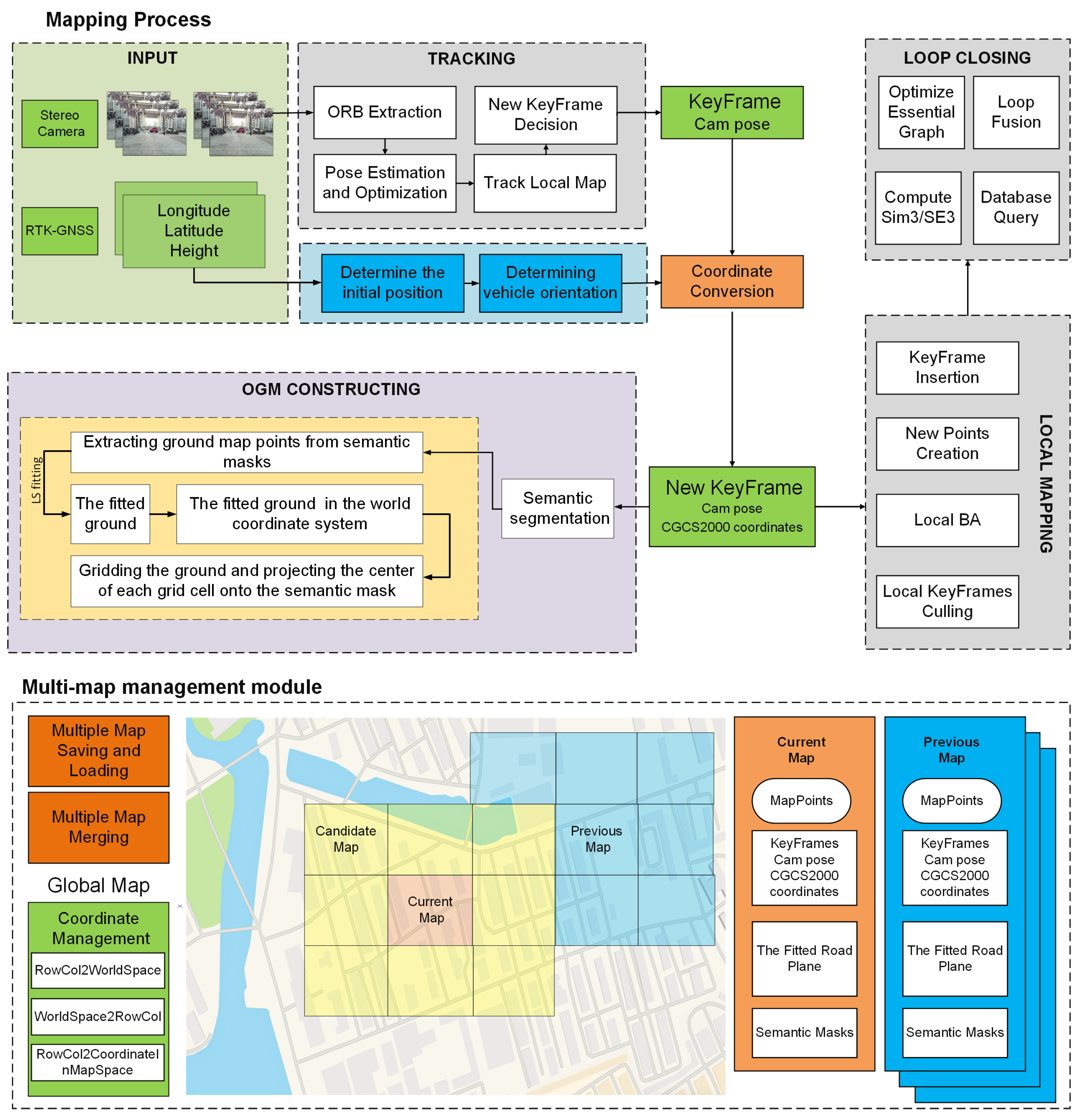
In recent years, many researchers have used RGB-D cameras for dense depth reconstruction to generate navigational grid maps, representing scene geometry through high-density 3D point clouds [7,8,9]. RGB-D cameras, based on the principle of active optical ranging, achieve real-time acquisition of pixel-level depth perception data by directly measuring the phase or time delay of signals reflected from object surfaces. These hardware characteristics enable RGB-D visual SLAM systems to establish dense 3D environments through direct physical measurements without relying on complex stereo matching algorithms. KinectFusion [7] is a milestone work and serves as a representative example. It achieves pose estimation and dense point cloud registration through the Iterative Closest Point (ICP) algorithm and introduces the Truncated Signed Distance Function (TSDF) for global optimization and incremental fusion of scene surfaces. This work validated the feasibility of RGB-D cameras in high-precision environment modeling and provided a significant reference for subsequent vision-based SLAM and navigational map construction. SemanticFusion [8] introduces semantic understanding into SLAM by fusing pixel-wise semantic segmentation from deep learning models with spatial mapping. By accumulating and refining semantic labels over time, it enhances scene comprehension and improves robustness in complex environments. MaskFusion [9] further extends this framework by incorporating instance-level segmentation, allowing the system to distinguish different elements in the environment. Using deep-learning-based instance masks, it refines the classification and representation of various regions, improving contextual awareness. Reference [25] proposed an improved real-time indoor localization system based on ORB RGB-D SLAM. While generating an ORB-SLAM sparse feature map, the system utilizes camera poses estimated by visual SLAM and laser scan data extracted from point clouds to construct and continuously update a 2D grid map in real time.

Dense depth estimation using stereo cameras can also be used to mapping, and in recent years, a number of stereo matching algorithms have appeared to obtain depth maps of entire images. Reference [26] employed a variational autoencoder (VAE) to improve stereo matching by learning a probabilistic disparity distribution. However, this method is computationally expensive in both training and inference and struggles with disparity estimation in low-texture and occluded regions. Reference [27] utilized cascaded residual learning to refine disparity estimation by incorporating contextual information. While it performs well in recovering fine details, its high computational complexity limits its scalability, particularly in large-scale scenes and under extreme lighting conditions. Reference [28] enhanced stereo matching by using an iterative geometry encoding volume (IGEV) to refine disparity estimation. While it improves accuracy, it remains computationally intensive and slow, limiting real-time applicability. Like other deep learning methods, it struggles with low-texture regions and occlusions. Reference [29] employed a real-time stereo matching network using Spatial Attention-Guided Upsampling to refine cost volumes and disparity maps, preserving high-frequency details and depth discontinuities. While it improves accuracy and efficiency, it may struggle with occlusions and low-texture regions, and its attention mechanisms could lead to higher memory consumption and potential artifacts in complex scenes. Unlike the above methods, our method does not calculate the depth value of each pixel in the whole image when mapping, while fitting the plane by sparse points, and the number of data is significantly reduced. Furthermore, our approach can construct maps in real time in real environments.

3. System Overview

The proposed multi-submap fusion mapping framework based on semantic road surface fitting comprises two main components: the mapping module and the multi-submap management module. The system architecture is shown in Figure 1.

During the mapping phase, we first obtain sparse map points from the ORB-SLAM3 system, which are generated by feature extraction and matching in the visual SLAM process and contain 3D spatial information of the scene. These map points contain both ground and non-ground points (buildings, obstacles, etc.), so they need to be filtered to extract accurate ground feature points. We utilize a pretrained semantic segmentation model to semantically segment the current frame image to obtain pixel-level semantic labels, which include semantic masks for ground categories. The map points generated by ORB-SLAM3 are then projected into the current frame image to obtain the pixel coordinates of each map point on the image plane. For each map point projected to the image plane, we determine whether it belongs to the ground category by querying the semantic labels of the corresponding pixel locations in the semantic segmentation result, and if so, these map points are retained; otherwise, they will be excluded. Subsequently, we model the ground in the scene to fit the plane to the point set composed of these ground points. After obtaining the ground plane model, we rasterize this plane into uniform raster cells, and considering the balance between map resolution and computational efficiency, we set the raster size to 0.1 m × 0.1 m.

We also propose a multi-submap management module to represent large scenes using multiple submaps. This module implements dynamic loading and storing of submaps as the vehicle position changes, as well as integration between multiple submaps. This approach is chosen because, when the automated guided vehicle (AGV) moves far from the origin of the world coordinate system, it is often impossible to obtain the occupancy status of every grid cell on the ground when attempting to map the entire scene at once. Furthermore, when the scene has a relatively large scale, loop closure detection and graph optimization [30] can cause significant changes in the poses of many keyframes, requiring large-scale adjustments to the grid map to reflect these changes. This process is highly time-consuming. In practical applications, operations such as reading and modifying the entire map of a scene may not meet the real-time requirements of system operation.

4. Methods

In navigation tasks, neural networks for dense depth estimation can reconstruct precise obstacle locations within a scene. However, for navigation purposes, reconstructing excessive surface details of obstacles is time-consuming and unnecessary, and it consumes substantial computational resources. This is particularly problematic in outdoor environments, where roads often occupy a large portion of the field of view. Furthermore, neural-network-based depth estimation tends to produce significant errors in areas with low texture, such as road surfaces. To address this problem, we employ semantic segmentation to extract ground features from the input image, fit a plane using the identified points, and designate the resulting plane as the ground. This plane is then rasterized, and the ground grid in the global coordinate system is reconstructed through back-projection [31]. Consequently, we generate a 2D occupancy grid map for navigation based on 3D point cloud data. The primary reason for choosing this map representation is that a 2D grid map transforms continuous space into a structured 2D array or matrix, providing directly interpretable input data (e.g., array indices) for path-planning algorithms.

The algorithm framework for the grid map construction module is shown in Figure 2. First, keyframes are extracted from the red-green-blue (RGB) image sequence using ORB-SLAM3. Semantic segmentation is then applied to generate a semantic mask for each keyframe, from which map points corresponding to the ground semantic region are identified. These map points are used to estimate the position of the road surface. Finally, the fitted road surface is rasterized, and the occupancy probability of each grid cell is determined through back-projection. This probability is continuously updated as the robot moves.

The ground to be fitted during map construction is derived from the point cloud in keyframes. However, in practical applications, it is unnecessary to wait for the tracking thread to extract keyframes before performing semantic segmentation. Therefore, an independent thread is designed to perform semantic segmentation on the input images, extracting the semantic masks corresponding to keyframes. This approach improves the real-time performance of the algorithm.

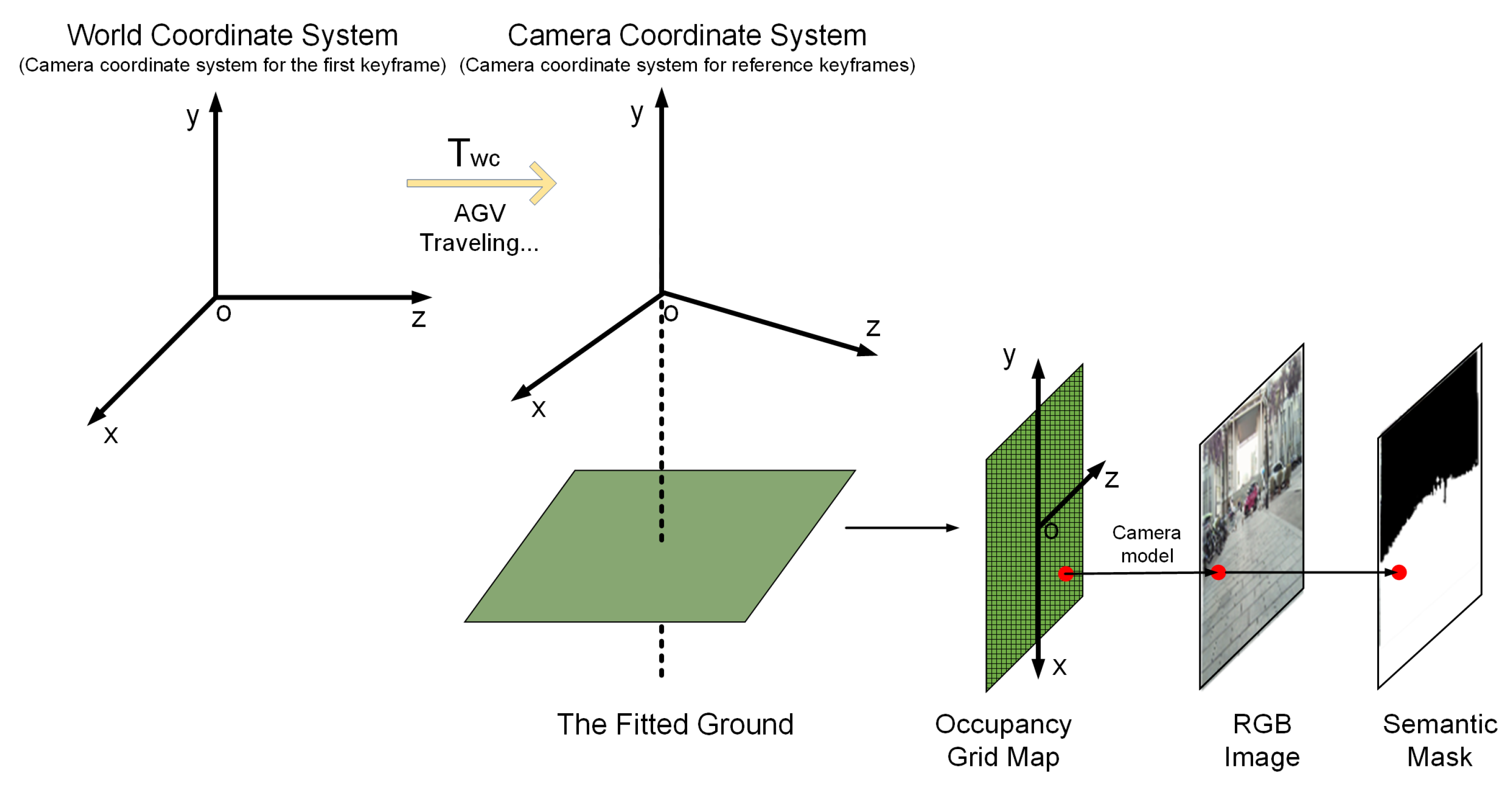
4.1. Incremental Ground Position Estimation

First, the semantic mask of the keyframe is obtained using PanopticFCN. The regions labeled “Road” and “Pavement” in the semantic mask are selected as candidate ground areas. To ensure that the point cloud is assigned an accurate semantic information, the semantic mask is first aligned with the keyframe’s scale. It is then assumed that a map point P exists in the point cloud, corresponding to a total of $n_k$ features. The pixel coordinates of these $n_k$ features are used to locate their positions in the semantic mask. If $m_k$ of these features are located within the ground semantic region of the mask, and if $n_k⩾3$ and ${\displaystyle \frac{m_k}{n_k}}>0.5$, the 3D coordinates of the map point P are calculated using the 2D pixel coordinates of the $m_k$ features. The map point P is then assigned the semantic attribute of the ground. This process results in a sparse point cloud with semantic information. The map points with ground semantics are filtered out to form a ground point cloud set, denoted as $S_f$, where $S_f=\left\{{\mathit{p}}_i\right\}\left(i=1,2,\dots ,m\right)$. If the number of map points in the ground point cloud does not exceed a given threshold, or if the points are too narrowly distributed, new keyframes and map points are generated. Otherwise, the initial estimate of the ground plane is made based on $S_f$. The fitted plane is represented using the Hessian normal form:

$${\mathit{n}}^{\mathrm{T}}\mathit{p}-d=0$$

(1)

where $\mathit{p}$ is a 3D row vector representing the coordinates of a point on the plane, $\mathit{n}$ is the unit normal vector of the plane, pointing from the origin of the coordinate system toward the plane, and $d\left(d>0\right)$ is the distance from the origin to the plane. During the movement of the AGV, only a portion of the ground point cloud within the camera’s field of view can be observed in the initial phase of system operation. This limited ground point cloud is insufficient for accurate plane fitting, making it difficult to construct a correct grid map. The key to achieving incremental online plane fitting is the algorithm’s ability to effectively leverage results from previous computations. The complete steps are shown in Algorithm 1. Suppose that during a given observation, a certain number of new ground map points are observed. The set of these newly observed ground map points is denoted as $S_f^{new}$, $S_f^{new}=\left\{{\mathit{p}}_j^{new}\right\}\left(j=1,2,\dots ,n\right)$. Let the combined point set, containing both the original ground map points and the newly observed points, be denoted as $S_f^{total}$, where $S_f^{total}=S_f\cup S_f^{new}$. The midpoint ${\mathit{p}}_c^{new}$ and variance $Var\left(S_f^{new}\right)$ of the point set $S_f^{new}$ are calculated. The midpoint ${\mathit{p}}_c^{total}$ and variance $Var\left(S_f^{total}\right)$ of the point set $S_f^{total}$ can then be computed as follows:

$${\mathit{p}}_c^{total}={\displaystyle \frac{m}{m+n}}{\mathit{p}}_c+{\displaystyle \frac{n}{m+n}}{\mathit{p}}_c^{new}$$

(2)

We define the variance of the point set $S_f^{total}$ as:

$$\begin{array}{cc}\hfill Var\left(S_f^{total}\right)& ={\displaystyle \frac{1}{m+n}}\sum _{{\mathit{p}}_i\in S_f}({\mathit{p}}_i-{\mathit{p}}_c^{total}){({\mathit{p}}_i-{\mathit{p}}_c^{total})}^{\mathrm{T}}+\hfill \\ \hfill & {\displaystyle \frac{1}{m+n}}\sum _{{\mathit{p}}_j^{new}\in S_f^{new}}({\mathit{p}}_j^{new}-{\mathit{p}}_c^{total}){({\mathit{p}}_j^{new}-{\mathit{p}}_c^{total})}^{\mathrm{T}}\hfill \end{array}$$

(3)

Split $\mathit{p}-{\mathit{p}}_c^{total}$ as follows:

$$\mathit{p}-{\mathit{p}}_c^{total}=(\mathit{p}-{\mathit{p}}_c)+({\mathit{p}}_c-{\mathit{p}}_c^{total})$$

(4)

For ${\sum }_{{\mathit{p}}_i\in S_f}({\mathit{p}}_i-{\mathit{p}}_c^{total}){({\mathit{p}}_i-{\mathit{p}}_c^{total})}^{\mathrm{T}}$, we have:

$$\sum _{{\mathit{p}}_i\in S_f}({\mathit{p}}_i-{\mathit{p}}_c^{total}){({\mathit{p}}_i-{\mathit{p}}_c^{total})}^{\mathrm{T}}=mVar\left(S_f\right)+m({\mathit{p}}_c-{\mathit{p}}_c^{total}){({\mathit{p}}_i-{\mathit{p}}_c^{total})}^{\mathrm{T}}$$

(5)

Similarly, after the transformation of Equation (4), we can get:

$$\begin{array}{cc}\hfill & \sum _{{\mathit{p}}_j^{new}\in S_f^{new}}({\mathit{p}}_j^{new}-{\mathit{p}}_c^{total}){({\mathit{p}}_j^{new}-{\mathit{p}}_c^{total})}^{\mathrm{T}}\hfill \\ \hfill & =\sum _{{\mathit{p}}_j^{new}\in S_f^{new}}({\mathit{p}}_j^{new}-{\mathit{p}}_c){({\mathit{p}}_j^{new}-{\mathit{p}}_c)}^{\mathrm{T}}+\hfill \\ & \sum _{{\mathit{p}}_j^{new}\in S_f^{new}}2({\mathit{p}}_c-{\mathit{p}}_c^{total}){({\mathit{p}}_j^{new}-{\mathit{p}}_c)}^{\mathrm{T}}+n({\mathit{p}}_c-{\mathit{p}}_c^{total}){({\mathit{p}}_c-{\mathit{p}}_c^{total})}^{\mathrm{T}}\hfill \end{array}$$

(6)

Let $\Delta {\mathit{p}}_c={\mathit{p}}_c^{total}-{\mathit{p}}_c$, and combined with Equations (3), (5), and (6), the final equation can be obtained:

$$\begin{array}{c}\hfill Var\left(S_f^{total}\right)={\displaystyle \frac{m}{m+n}}Var\left(S_f\right)+\Delta {\mathit{p}}_c\Delta {\mathit{p}}_c^{\mathrm{T}}+\\ \hfill {\displaystyle \frac{{\displaystyle \sum _{j=1}^n\left[({\mathit{p}}_j^{new}-{\mathit{p}}_c){({\mathit{p}}_j^{new}-{\mathit{p}}_c)}^{\mathrm{T}}-2\Delta {\mathit{p}}_c{({\mathit{p}}_j^{new}-{\mathit{p}}_c)}^{\mathrm{T}}\right]}}{m+n}}\end{array}$$

(7)

Algorithm 1 Incremental Calculation of Fitted Ground Plane Parameters

Input:  The midpoint ${\mathit{p}}_c$ and variance $Var\left(S_f\right)$ from the previous execution of Algorithm 1, and the newly observed ground map point set $S_f^{new}$. Output:  The normal vector $\mathit{n}$ of the fitted plane and the distance d from the plane to the origin.  1: Compute the midpoint ${\mathit{p}}_c^{new}$ of the point set $S_f^{new}$: $${\displaystyle {\mathit{p}}_c^{new}=\frac{1}{n}\sum _{j=1}^n{\mathit{p}}_j^{new}\left({\mathit{p}}_j^{new}\in S_f^n,j=1,2,\dots ,n\right)}$$ (8)  2: Compute the midpoint ${\mathit{p}}_c^{total}$ and variance $Var\left(S_f^{total}\right)$ of the point set $S_f^{total}=S_f\cup S_f^{new}$ using Equations (2) and (7).  3: Perform Singular Value Decomposition (SVD) on the variance $Var\left(S_f\right)$, and select the right singular vector corresponding to the smallest singular value as the normal vector $\mathit{n}$ of the fitted plane.  4: Compute the distance d from the origin to the fitted ground plane.  5: Calculate the standard deviation $\sigma$ of the distances from the point set to the fitted ground plane.  6: If the standard deviation $\sigma$ is less than the given threshold, assign ${\mathit{p}}_c^{total}$ and variance $Var\left(S_f^{total}\right)$ to ${\mathit{p}}_c$ and $Var\left(S_f\right)$, respectively, for storage, and terminate the algorithm. If $\sigma$ is greater than the given threshold, proceed to step 7. $${\mathit{p}}_c:={\mathit{p}}_c^{total}$$ (9) $$Var\left(S_f\right):=Var\left(S_f^{total}\right)$$ (10)  7: Points with distances greater than $\sigma$ from the fitted ground plane are considered outliers and are removed, while points with distances less than $\sigma$ are considered inliers and are retained. The retained inliers are then used to reconstruct the point set $S_f$. Steps 2 to 6 are repeated thereafter.

It can be observed that, when updating the fitted ground plane parameters, the algorithm only requires incorporating the previously computed ${\mathit{p}}_c$, $Var\left(S_f\right)$, and the newly observed ground map point set $S_f^{new}$ into the calculations. The originally observed ground map point set $S_f$ is not needed. This approach ensures a stable time complexity for the plane fitting update, thus improving the efficiency of the mapping system in outdoor scenarios.

4.2. Multi-Submap Fusion Mapping Method for Outdoor Environment

When the AGV traverses a certain distance, the road surface in the actual environment may display varying slopes, making it impractical to fit the entire ground into a single ideal plane. Moreover, loop closure detection and pose graph optimization in relatively large environments can significantly alter the poses of many keyframes, necessitating extensive adjustments to the grid map, which is highly time-consuming. Operations such as reading, modifying, and updating maps for an entire scene may also fail to meet the system’s real-time requirements. To address these challenges, a multi-submap approach is adopted to represent relatively large environments. Submaps are created or retrieved based on the robot’s current location, while historical maps are stored for future use. Notably, our system transforms the SLAM coordinate system into the Chinese Geodetic Coordinate System 2000 (CGCS2000) [32], allowing the fusion and integration of our maps with any others constructed using CGCS2000 coordinates.

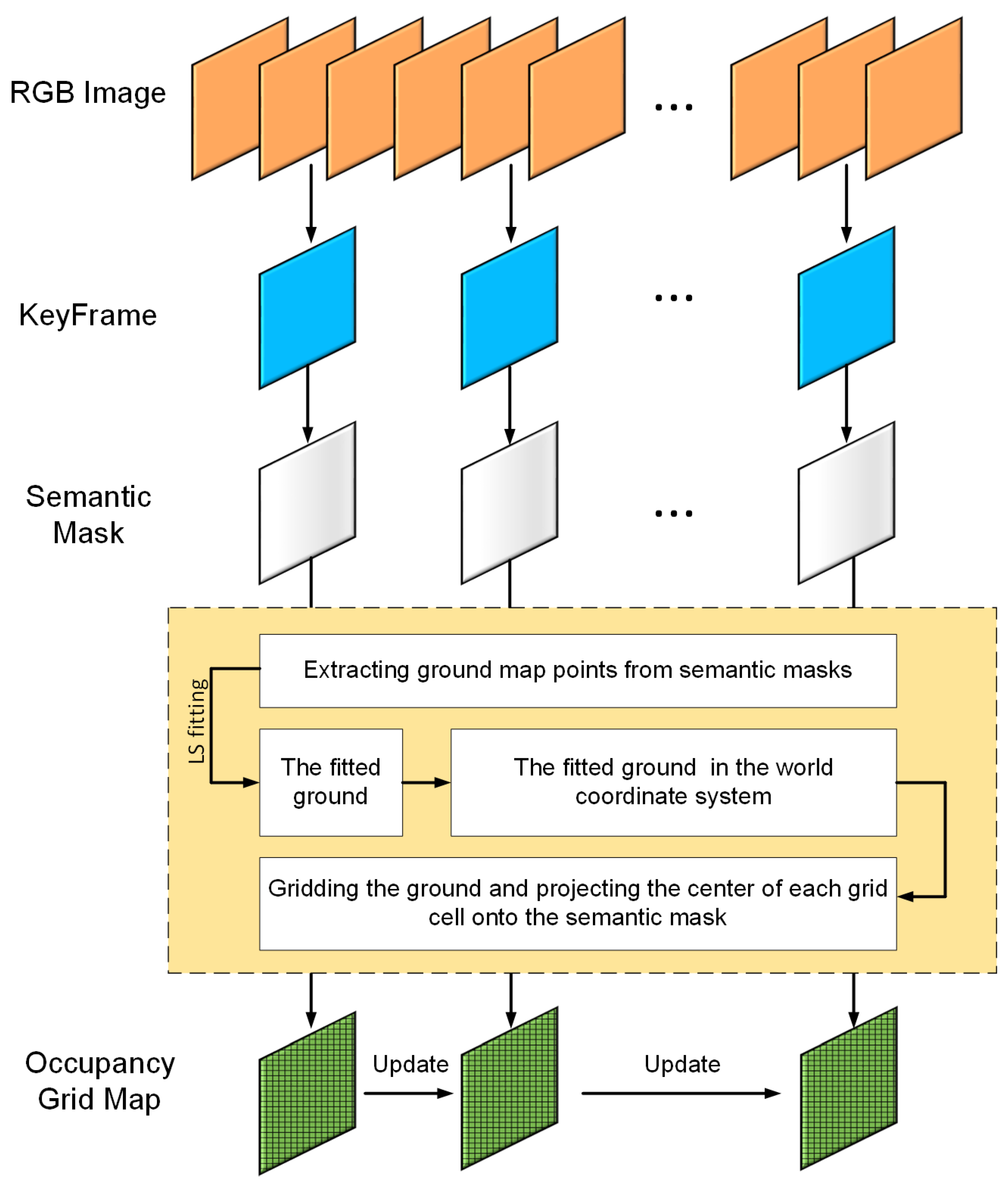
4.2.1. Map Update Strategy for a Single Submap

We set the area covered by each submap to 10 m × 10 m, with each submap associated with a reference keyframe. When generating a new submap centered at a given location, the keyframe nearest to this center is selected as the reference using the pose matrix. In ORB-SLAM3, the system adopts the camera coordinate system of the first keyframe generated after initialization as the world coordinate system. Let the pose of the reference keyframe be denoted as ${\mathit{T}}_{\mathit{wc}}$; the ground plane fitted from the ground map points has a plane equation in the camera coordinate system of this reference keyframe as follows:

$${\mathit{n}}_c^{\mathrm{T}}\mathit{p}-d_c=0$$

(11)

where ${\mathit{n}}_c$ represents the unit normal vector of the fitted ground plane in the camera coordinate system of the current reference keyframe and $d_c$ denotes the distance from the origin of this camera coordinate system to the fitted ground plane. Both parameters can be obtained through the incremental ground plane fitting algorithm mentioned earlier.

Since the pose of the reference keyframe is ${\mathit{T}}_{\mathit{wc}}$, the normal vector ${\mathit{n}}_w$ of the fitted ground plane in the world coordinate system can be calculated using the following Equation (12) in the camera coordinate system of the reference keyframe:

$$\left(\begin{array}{c}{\mathit{n}}_w\\ 0\end{array}\right)={\mathit{T}}_{\mathit{wc}}\left(\begin{array}{c}{\mathit{n}}_c\\ 0\end{array}\right)$$

(12)

Let $P_{prj}$ denote the projection of the origin of the camera coordinate system of the reference keyframe onto the fitted ground plane, with coordinates ${\mathit{p}}_{prjc}$. The corresponding coordinates ${\mathit{p}}_{prjw}$ in the world coordinate system can be determined using the following Equation (13):

$$\left(\begin{array}{c}{\mathit{p}}_{prjw}\\ 0\end{array}\right)={\mathit{T}}_{\mathit{wc}}\left(\begin{array}{c}{\mathit{p}}_{prjc}\\ 0\end{array}\right)$$

(13)

From Equation (14), the distance $d_w$ from the fitted ground plane to the origin of the world coordinate system, as expressed in the camera coordinate system of the reference keyframe, can be written as follows:

$$d_w={\mathit{n}}_w^{\mathrm{T}}{\mathit{p}}_{prjw}$$

(14)

If $d_w$ is negative, both the normal vector ${\mathit{n}}_w$ and the distance $d_w$ should be inverted. If $d_w$ is positive, no inversion is required. Consequently, the plane equation of the ground surface in the world coordinate system for the submap can be written as follows:

$${\mathit{n}}_w^{\mathrm{T}}\mathit{p}-d_w=0$$

(15)

After determining the parameters of the fitted ground plane, a reference coordinate system for the occupancy grid map must be established. To facilitate subsequent mapping, a three-dimensional coordinate system is chosen as the reference. This system is defined such that the fitted ground plane corresponds to the xOy-plane, with the Z-axis oriented upwards from the plane. This coordinate system will henceforth be referred to as the submap coordinate system. Since the relative position between the submap and the world coordinate systems is fixed, the transformation between them can be easily derived. The transformation from the submap coordinate system to the world coordinate system is denoted as ${\mathit{T}}_{ws}$.

The center of the submap is defined as the origin of the submap coordinate system. Since each submap has the same scale and resolution, the distance between the centers of two adjacent submaps is fixed. Therefore, the projected position of each submap’s center on the xOz-plane of the world coordinate system can be determined, with the projection coordinates denoted as ${\left(X_{SubMap},Z_{SubMap}\right)}^{\mathrm{T}}$. To determine the coordinates ${\left(X_{SubMap},Y_{SubMap},Z_{SubMap}\right)}^{\mathrm{T}}$ of the center of the submap in the world coordinate system, it is sufficient to compute its component along the Y-axis, denoted as $Y_{SubMap}$. This value can then be substituted into the fitted ground plane equation to obtain the following:

$$\left(\begin{array}{ccc}{n}_{wx}& n_{wy}& n_{wz}\end{array}\right)\left(\begin{array}{c}{X}_{SubMap}\\ Y_{SubMap}\\ Z_{SubMap}\end{array}\right)-d_w=0$$

(16)

where $\left(n_{wx},n_{wy},n_{wz}\right)$ is equivalent to ${\mathit{n}}_w^{\mathrm{T}}$. By rearranging the equation, $Y_{SubMap}$ can be computed, which allows for the determination of the world coordinates of the submap center as follows:

$$Y_{SubMap}={\displaystyle \frac{d_w-n_{wx}{X}_{SubMap}-n_{wz}{Z}_{SubMap}}{n_{wy}}}$$

(17)

Let the center coordinates of the submap, denoted as ${\left(X_{SubMap},Y_{SubMap},Z_{SubMap}\right)}^{\mathrm{T}}$, be represented by ${\mathit{p}}_{submap}$, and the coordinates of the submap center in the CGCS2000 coordinate system, denoted as ${\mathit{p}}_{CGCS}$, where ${\mathit{p}}_{CGCS}={\left(X_{CGCS},Y_{CGCS},Z_{CGCS}\right)}^{\mathrm{T}}$. Let the initial orientation of the vehicle relative to the longitudinal axis of the CGCS2000 coordinate system be denoted as $\theta$. The following equation holds:

$$\left[\begin{array}{c}{X}_{CGCS}\\ Y_{CGCS}\\ 1\end{array}\right]=\left[\begin{array}{ccc}cos\theta & -sin\theta & x_0\\ sin\theta & cos\theta & y_0\\ 0& 0& 1\end{array}\right]\left[\begin{array}{c}{X}_{SubMap}\\ Y_{SubMap}\\ 1\end{array}\right]$$

(18)

By using Equation (18), we align the map center coordinates between the relative coordinate system and the CGCS2000 coordinate system, thereby determining the position of each grid cell in the CGCS2000 coordinate system. On the xOz-plane of the submap coordinate system, we sample a series of points at 0.1 m intervals across the entire plane. The resulting array of points represents the centers of each grid cell in the submap. The coordinates of these points in the submap coordinate system, denoted as ${\mathit{p}}_{ij}$, can be expressed as:

$${\mathit{p}}_{ij}={\left(0.1i,0,0.1j\right)}^{\mathrm{T}}$$

(19)

where the variables i and j are both integers ranging from −50 to 50. When the AGV operates within the current submap’s range and new keyframes with their corresponding semantic masks are provided as input observations, we do not update all the grid cells of the submap simultaneously. To ensure precise updates of the grid cells’ occupancy status, we adopt a strategy of multiple small-scale updates. If the Chebyshev distance between the center of a grid cell and the keyframe in the xOz-plane of the submap coordinate system is less than 3 m, the grid cell is projected onto the semantic mask via the transformation matrix between the submap and camera coordinate systems. The specific projection process is illustrated in Figure 3.

First, the center of the grid cell is transformed from the submap coordinate system into the camera coordinate system. Using the camera’s intrinsic parameters, the pixel coordinates of the grid cell’s center are computed. The corresponding position on the semantic mask is then identified based on these pixel coordinates, thereby projecting the grid cell center onto the semantic mask. If the projected point falls within the mask region labeled as a road, the probability of the grid cell being classified as a “road cell” increases; otherwise, it decreases. As more keyframes are input, this probability is updated accordingly. Once the probability exceeds a predefined threshold, the grid cell is classified as a road cell. The detailed steps of the entire map update process are outlined in Algorithm 2.

Algorithm 2 Submap Update Using KeyFrame Observations

Input:  KeyFrame $pKF$, Map Transform $Twm$, Cell Length $sfCellLength$, Cell Radius $CellNearKFRadius$, Map Size $\left(snWidth,snHeight\right)$. Output:  Updated Submap Cells $mvCells$.  1: Obtain the current camera pose ${\mathit{T}}_{cw}$ from the reference keyframe.  2: Calculate the transformation matrix ${\mathit{T}}_{cm}={\mathit{T}}_{cw}·{\mathit{T}}_{wm}$ from the submap to the reference keyframe camera coordinate system.  3: Invert the transformation matrix ${\mathit{T}}_{cm}$ to obtain the transformation matrix ${\mathit{T}}_{mc}$ from the camera coordinate system to the submap coordinate system.  4: Create two variables, $fXInMapSpace$ and $fZInMapSpace$, to store the values representing the X and Z coordinates in the map coordinate system from ${\mathit{T}}_{cm}$.  5: Convert the map coordinates to grid indices $KFRowCol$.  6: Compute the range offset $nDeltaIdx$ based on $CellNearKFRadius$ and $sfCellLength$.  7: Determine the grid boundaries $nRowEnd$ and $nColEnd$.  8: Iterate through each grid cell within the grid range $\left(nRow,nCol\right)$.  9: Transform the center of the grid cell to the camera coordinate system.  10: Calculate the depth value and image coordinates $\left(u,v\right)$.  11: If $\left(u,v\right)$ is within the image range: If the mask value is valid, increase the corresponding $mvCells$ value. If the mask value is invalid, decrease the corresponding $mvCells$ value.  12: End the iteration and return the values of $mvCells$.

When new ground map points are introduced, they alter the parameters of the fitted ground plane, denoted as $\left(\mathit{n},d\right)$, which subsequently impacts the grid map. To maintain map accuracy, the grid map must be reconstructed whenever $\left(\mathit{n},d\right)$ changes significantly. We assume that the grid map was constructed based on the value of $\left({\mathit{n}}_s,d_s\right)$ during the last reconstruction. As the camera moves and more ground points are observed, the difference between the updated $\left(\mathit{n},d\right)$ (calculated using Algorithm 2) and the original $\left({\mathit{n}}_s,d_s\right)$ increases. When this difference exceeds a specified threshold, the error in the grid map constructed from $\left({\mathit{n}}_s,d_s\right)$ becomes unacceptable, thereby necessitating reconstruction.

In this study, two thresholds, $t_1$ and $t_2$, are defined to determine when grid map reconstruction is required. The conditions for reconstruction are as follows:

$${\mathit{n}}^{\mathrm{T}}{\mathit{n}}_s<t_1$$

(20)

$$∥d-d_s∥>t_2$$

(21)

Equations (20) and (21) represent the directional difference of the normal vectors and the distance difference between two planes, respectively. If either of these conditions is satisfied, $\left(\mathit{n},d\right)$ is assigned to $\left({\mathit{n}}_s,d_s\right)$, and the grid map is reconstructed based on the updated $\left({\mathit{n}}_s,d_s\right)$.

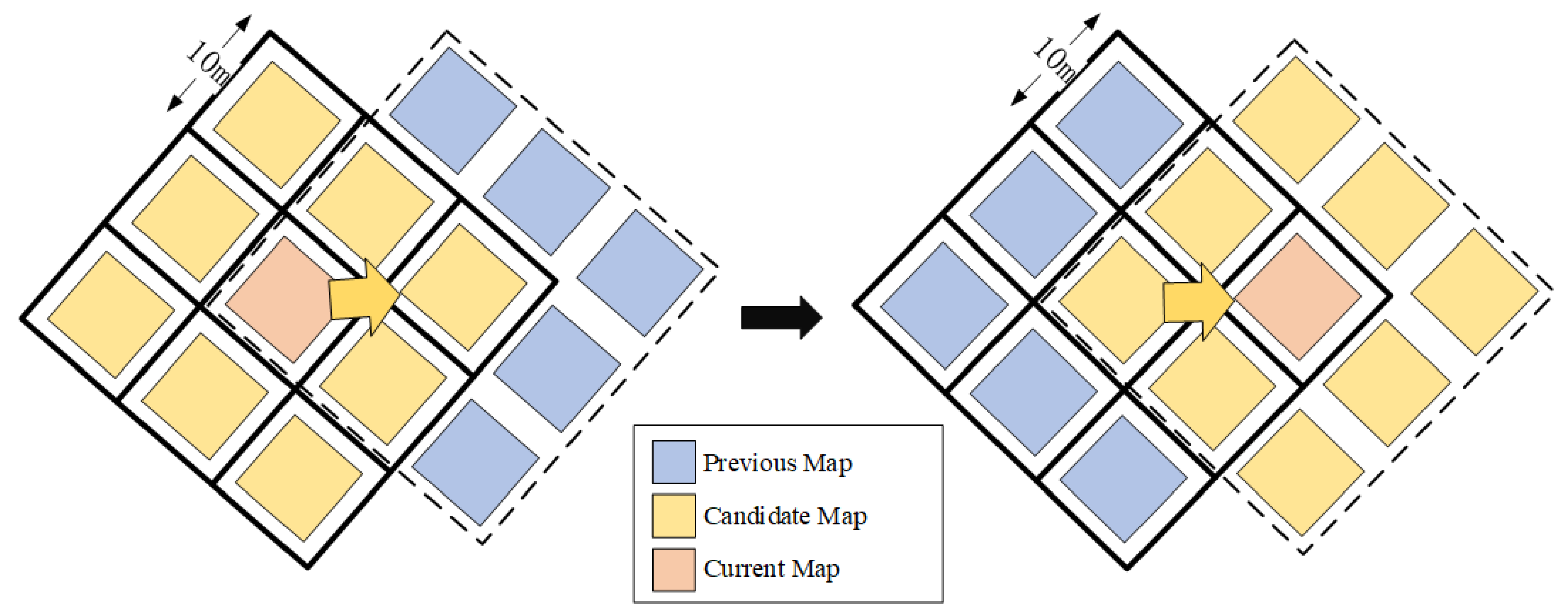
4.2.2. The Multi-Submap Management Module

In the previous section, we introduced the map update strategy for each submap. To represent large-scale environments using multiple submaps, we designed a multi-submap management module. During the initial stage of system operation, the vehicle’s central coordinates and orientation are measured using Real-Time Kinematic (RTK). These coordinates serve as the center for the first submap, and a submap is created at the vehicle’s current location. Simultaneously, eight additional submaps surrounding this central submap are established, as shown in Figure 4.

The entire submap object is stored as a binary file through serialization. The submap object contains attributes including the current map state, center coordinates, timestamp, and grid occupancy probabilities. When submap data are required, the object is restored via deserialization. To prevent interruptions in the SLAM system on the main thread, the storage and retrieval operations are executed on a separate thread. Moreover, to enhance lookup efficiency, a hash index is employed for submap storage. Because using floating-point numbers directly as keys can lead to precision errors, discretized integer coordinates of the submap center are used as the hash key. When a large number of submaps is present, it is impractical to keep all of them in memory; thus, the map states are categorized into three types: Current Map, Candidate Map, and Previous Map. The Current Map refers to the submap in which the vehicle is currently located and is retained in memory until the vehicle departs. The Candidate Map indicates the submap into which the vehicle is about to enter and must be preloaded into memory. The Previous Map consists of submaps that the vehicle has left, which are stored on the hard disk and reloaded only when necessary.

The state of each submap is dynamic and updates continuously as the vehicle moves. To reflect these changes, the attributes of the map object are modified as needed. Before generating a new submap, the map database is checked to determine whether an existing submap file already covers the vehicle’s current position. If no such submap exists, the system identifies the nearest submap center within the database and creates a new submap at that location. Next, eight surrounding candidate submaps are generated with uniformly spaced centers. If a submap covering the current position is already available in the database, it is loaded along with its eight adjacent submaps. When fewer than eight surrounding submaps are available, empty maps are generated to fill the gaps. The submap corresponding to the vehicle’s current position is designated as the “Current Map”, while the surrounding eight submaps are classified as “Candidate Maps”.

To achieve seamless representation of a large scene using multiple submaps, the algorithm ensures that adjacent submaps overlap during their generation. To model the connectivity between submaps, an adjacency graph is maintained, where each submap functions as a node. If two submaps share an overlapping edge region, an undirected edge is added to the graph. This adjacency graph is stored in a hash table to facilitate efficient querying. In this study, the edge region of a submap is defined as the area where the Euclidean distance from its center exceeds 0.9 of the submap’s radius. When the vehicle reaches the edge of the current submap, it checks whether an adjacent submap exists in the neighboring region. If present, a connectivity relationship is established; otherwise, a new submap is initialized, and the connectivity is recorded. Because grid occupancy probabilities in overlapping regions may vary between submaps, this study employs Bayesian updating in log-odds form to integrate these probabilities:

$$L\left(O\right)=\log {\displaystyle \frac{P\left(O\right)}{1-P\left(O\right)}}$$

(22)

where $P\left(O\right)$ represents the occupancy probability of a grid, while $1-P\left(O\right)$ denotes the probability that the grid is unoccupied. Let the occupancy probabilities of the same grid cell in submaps A and B be $P_A$ and $P_B$, respectively. According to the above equation, their corresponding log-odds values can be obtained as follows:

$$L_A=\log {\displaystyle \frac{P_A}{1-P_A}},L_B=\log {\displaystyle \frac{P_B}{1-P_B}}$$

(23)

Initially, the occupancy probability and the vacancy probability of the grid are equal, both being 0.5. Therefore, $L_0=0$. Under this assumption, the fused log-odds value is as follows:

$$L_{\mathrm{fused}}=L_A+L_B$$

(24)

Finally, the fused log-odds value is converted back to the occupancy probability, as follows:

$$P_{\mathrm{fused}}={\displaystyle \frac{1}{1+e^{-L_{\mathrm{fused}}}}}$$

(25)

We designate $P_{\mathrm{fused}}$ as the final occupancy probability of the overlapping grid cell.

5. Experimental Results

To evaluate the effectiveness and performance of the proposed algorithm, we used existing laboratory equipment and a self-constructed experimental platform. Representative real-world scenarios on campus were selected for mapping experiments, which demonstrated the algorithm’s validity.

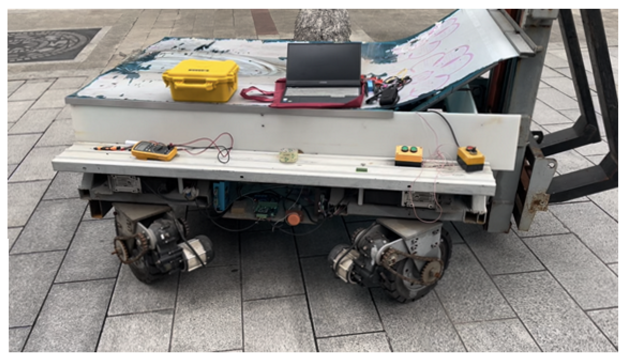
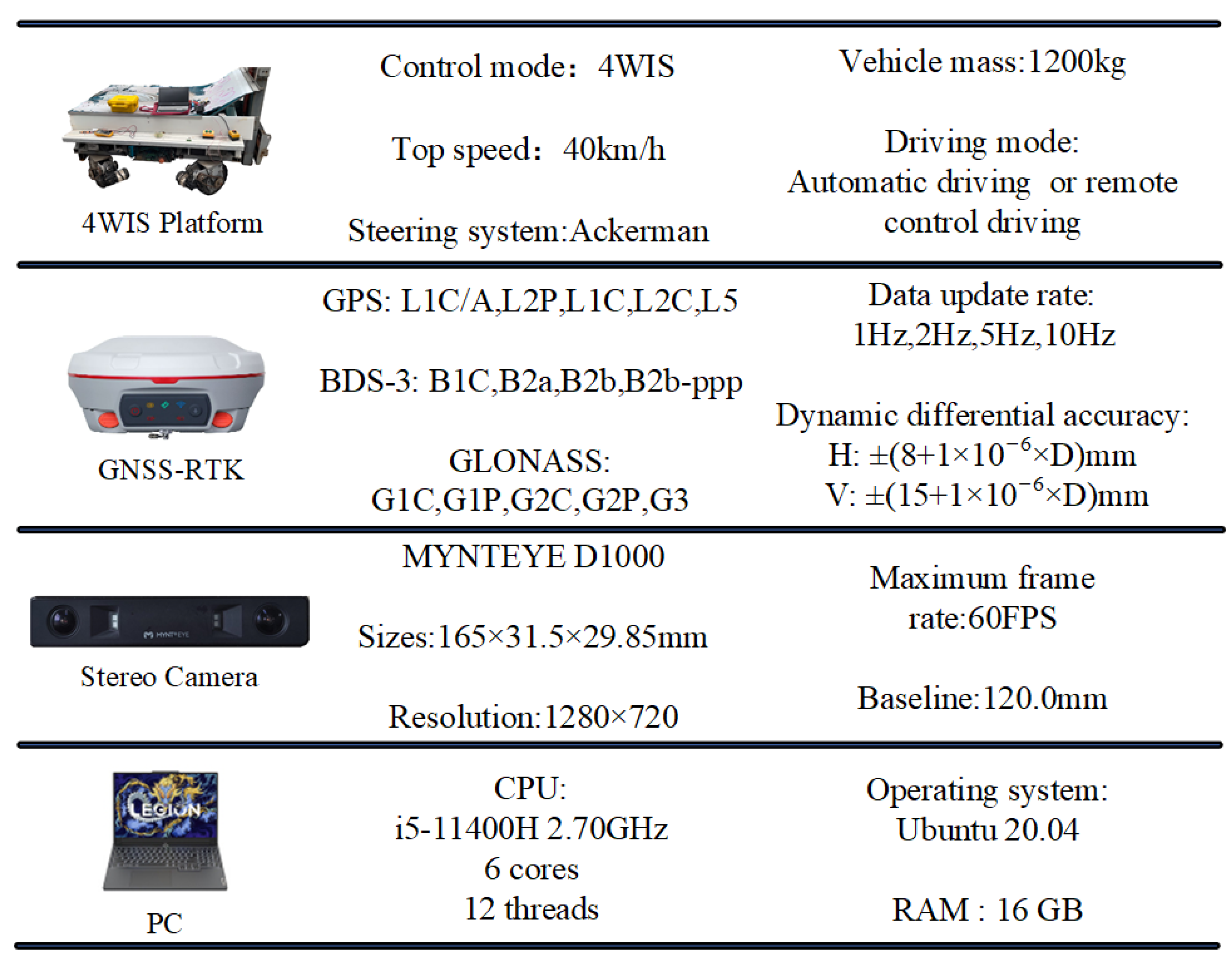
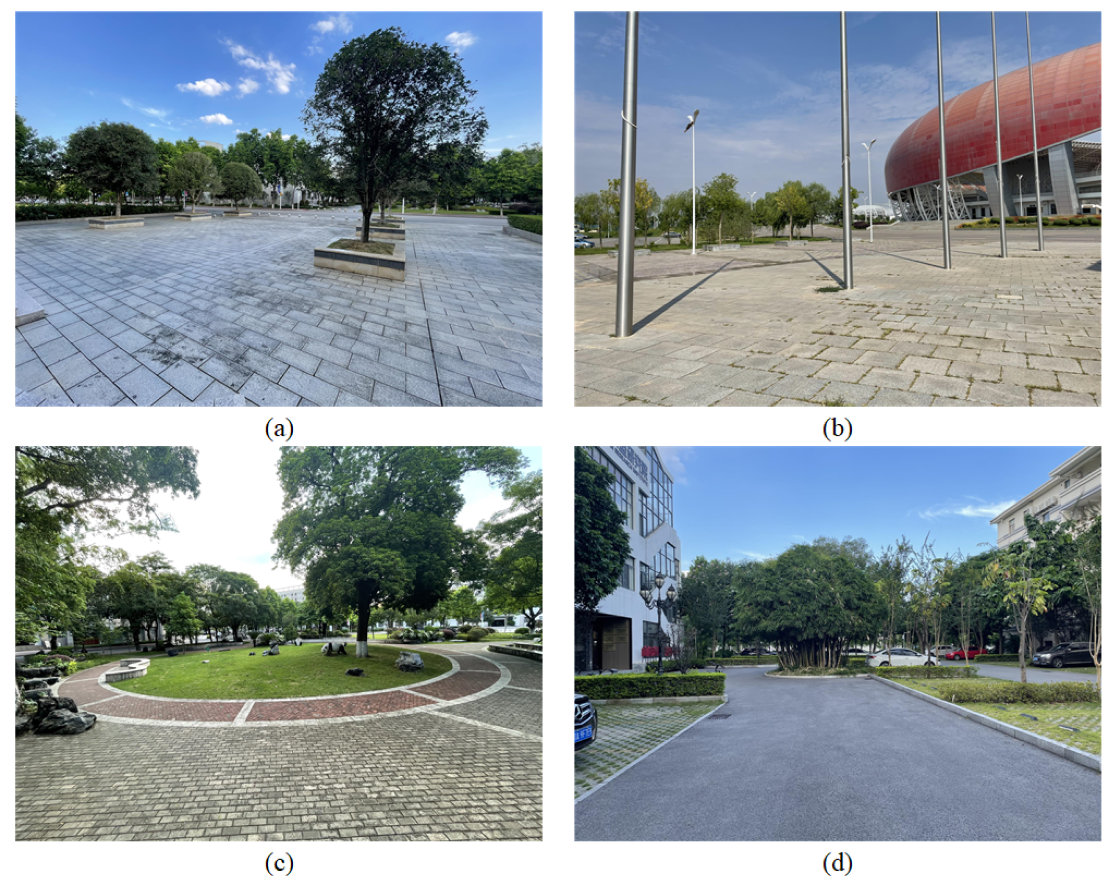
5.1. Experimental Setup and Environment

The experiments were conducted on a fully self-constructed experimental platform, as shown in Figure 5. The platform uses a four-wheel independent drive and four-wheel independent steering (4WID-4WIS) [33] control system, where each of the four wheels is equipped with independent steering and drive motors. A personal computer (PC) functions as the main controller, commanding the platform’s movement such as forward, backward, turning, and rotating in place via a mobile app. A stereo camera with a resolution of 1280 × 720 is mounted at the front of the platform, with an RTK measurement terminal positioned directly beneath it to determine the vehicle’s initial position and orientation, as well as to provide accurate RTK-measured landmark data. The specific details of the experimental setup are provided in Figure 6.

The experimental environment in real-world scenarios is shown in Figure 7. To ensure a variety of experimental conditions, four locations with different obstacles were selected. As depicted in Figure 7a, square flower beds with sides ranging from 1 to 2 m were chosen as obstacles. Figure 7b shows cylindrical flagpoles with a diameter of approximately 50 cm as obstacles. These two scenarios allow for the evaluation of the algorithm’s reconstruction performance on obstacles of varying sizes. Figure 7c,d depict two more complex terrains with minimal obstacles along the road surface. Since the algorithm primarily constructs the grid map by fitting the ground plane, these scenarios were selected to test the algorithm’s reconstruction capabilities for road surfaces.

During the experiment, the experimental platform was remotely controlled to move at a speed of 0.5 m/s while mapping the environment. When approaching obstacles, the speed was reduced to improve mapping accuracy. Throughout the experiment, true coordinates for every point on the road surface and obstacles could not be obtained. Since the primary application of the algorithm is to use the constructed map for path planning and enable autonomous navigation, it is unnecessary to acquire the true coordinates of all points as ground truth for map evaluation. Instead, the edges of obstacles and the road surface were selected as landmarks. Sampling was performed at these landmarks, and the true coordinates of the sampling points were measured using RTK, serving as ground truth for the map.

As shown in Figure 8, the green points represent the center of the free grid. The green areas denote traversable regions, whereas the black areas signify non-traversable regions. The mapping results in Figure 8 exhibit slight visual differences compared to Figure 9c, Figure 10c, Figure 11c and Figure 12c. This discrepancy arises because, in our visualization program, users can zoom in and out on the map using the middle mouse button. At higher zoom levels, discrete green grid centers become visible. However, for larger maps, we scale down the display to present the entire map, making individual grid centers indiscernible and instead forming a continuous green region. The resolution of the constructed grid map is known, with each grid cell measuring 0.1 m in length. Using the initial position coordinates and orientation of the experimental platform, obtained through RTK measurement, the true coordinates of any point in the grid map can be computed through simple calculations. Since the map is two-dimensional, minor errors in the vertical direction are acceptable. Mapping performance is evaluated by calculating the coordinates of selected landmark sampling points in the grid map and comparing them with the true coordinates to determine the error.

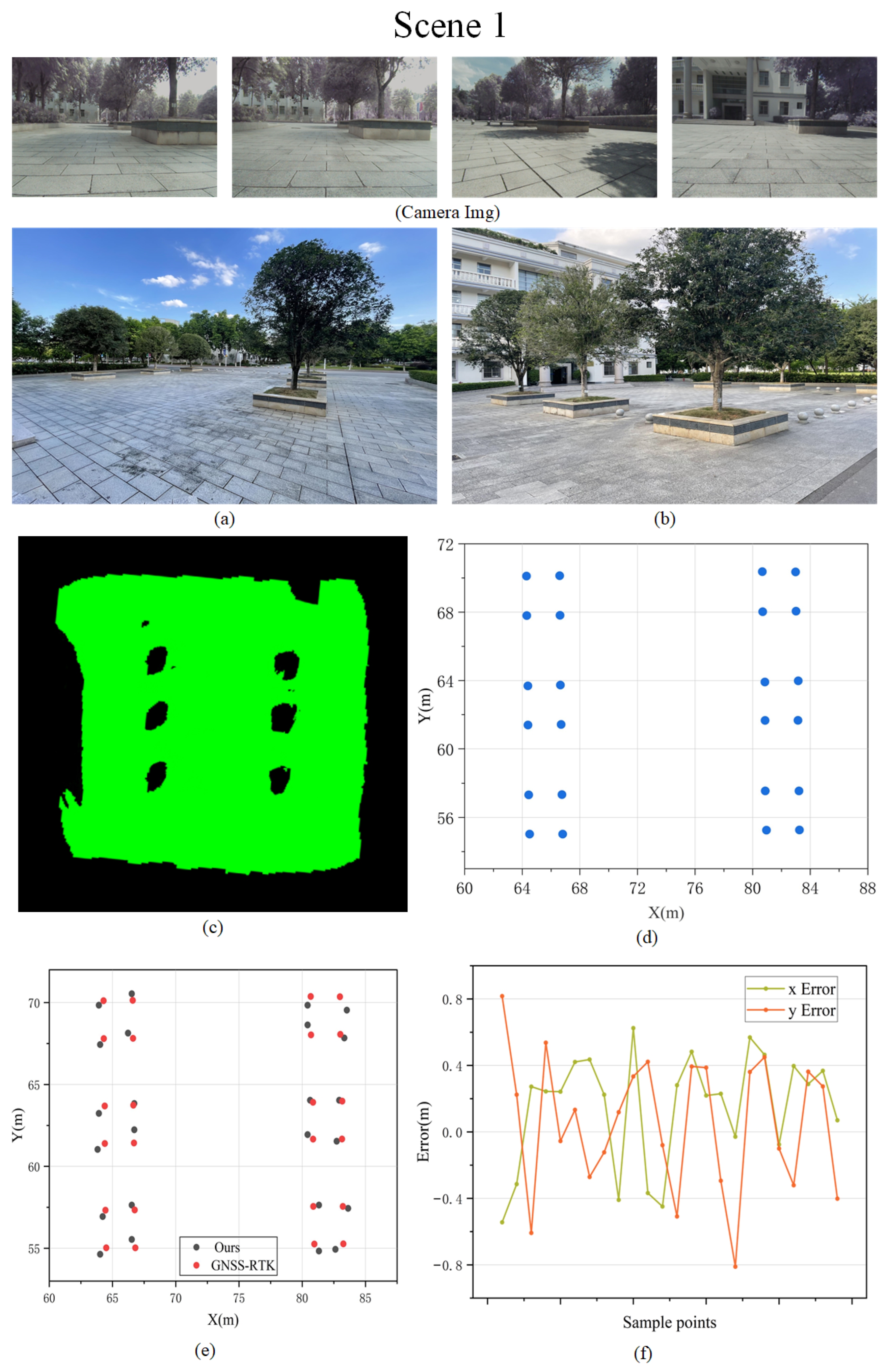
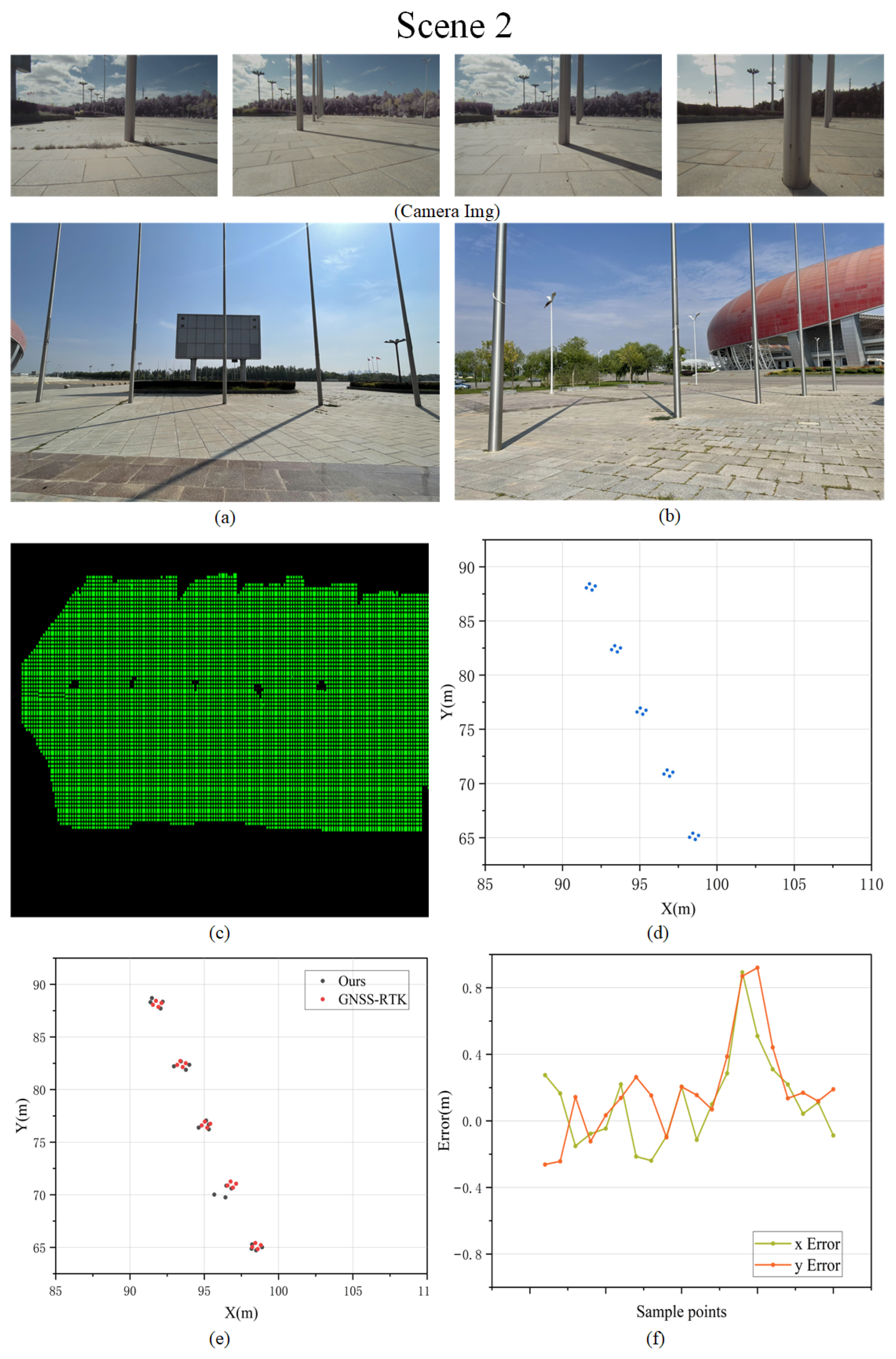
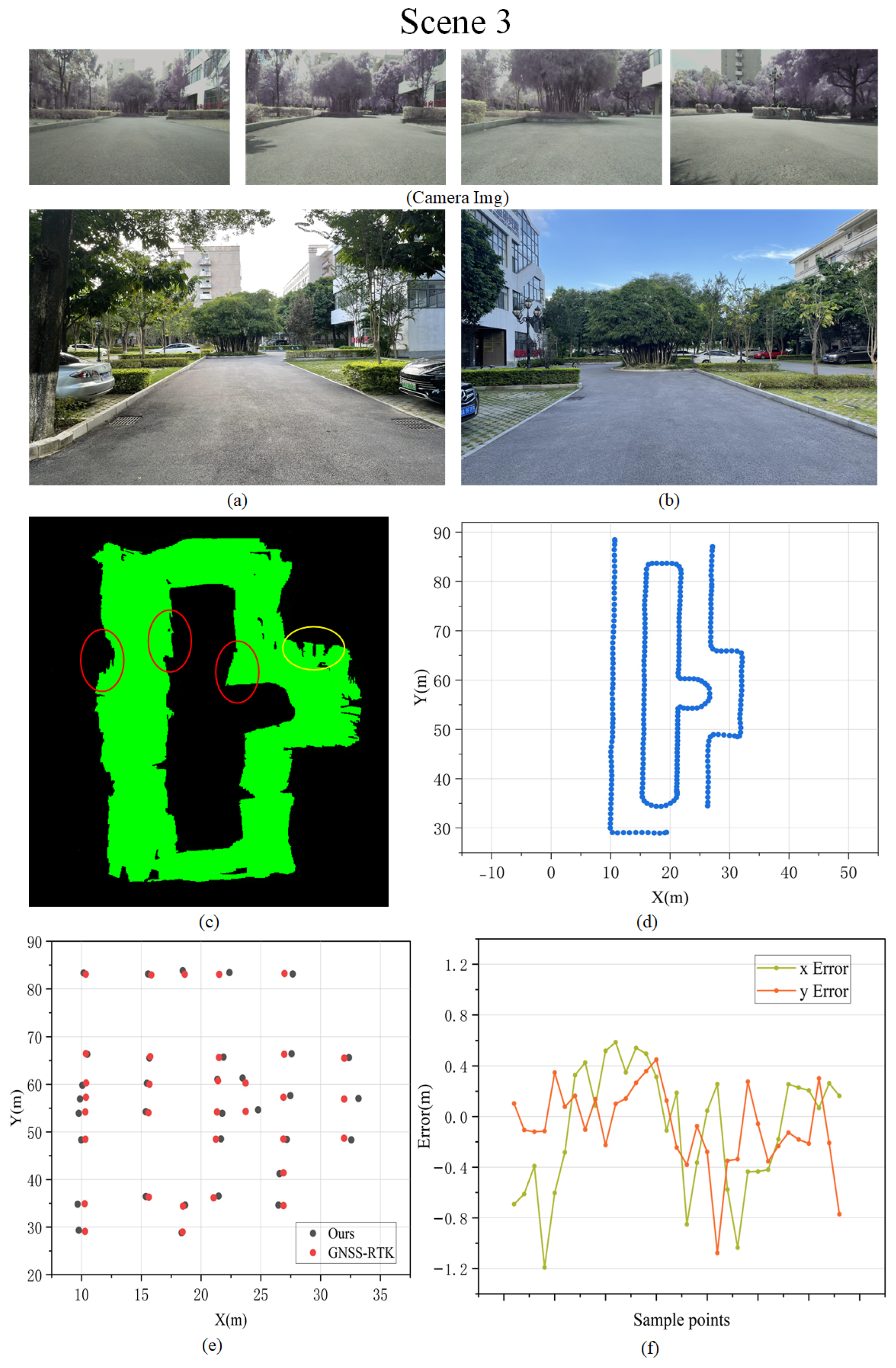
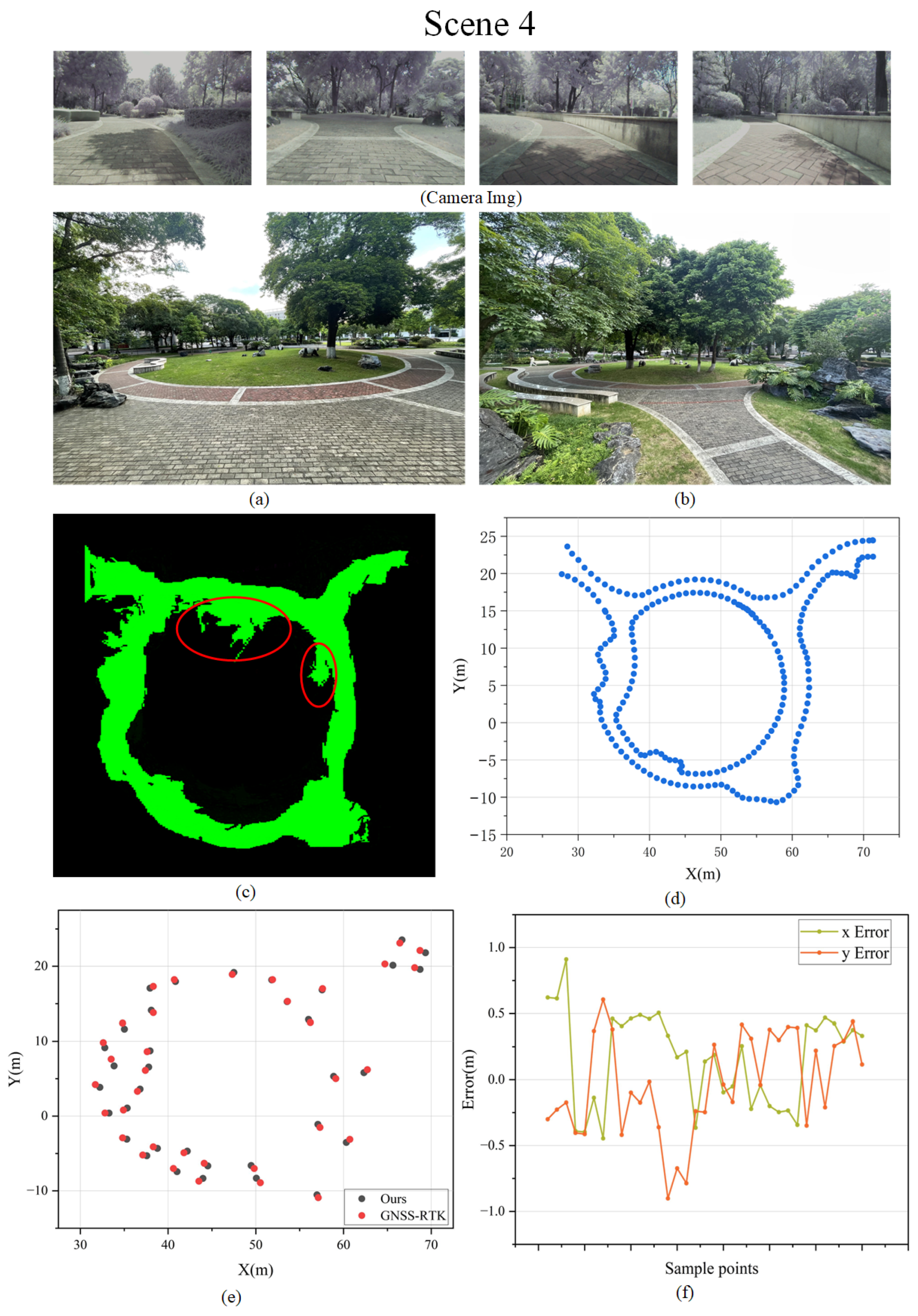
5.2. Experimental Results Analysis

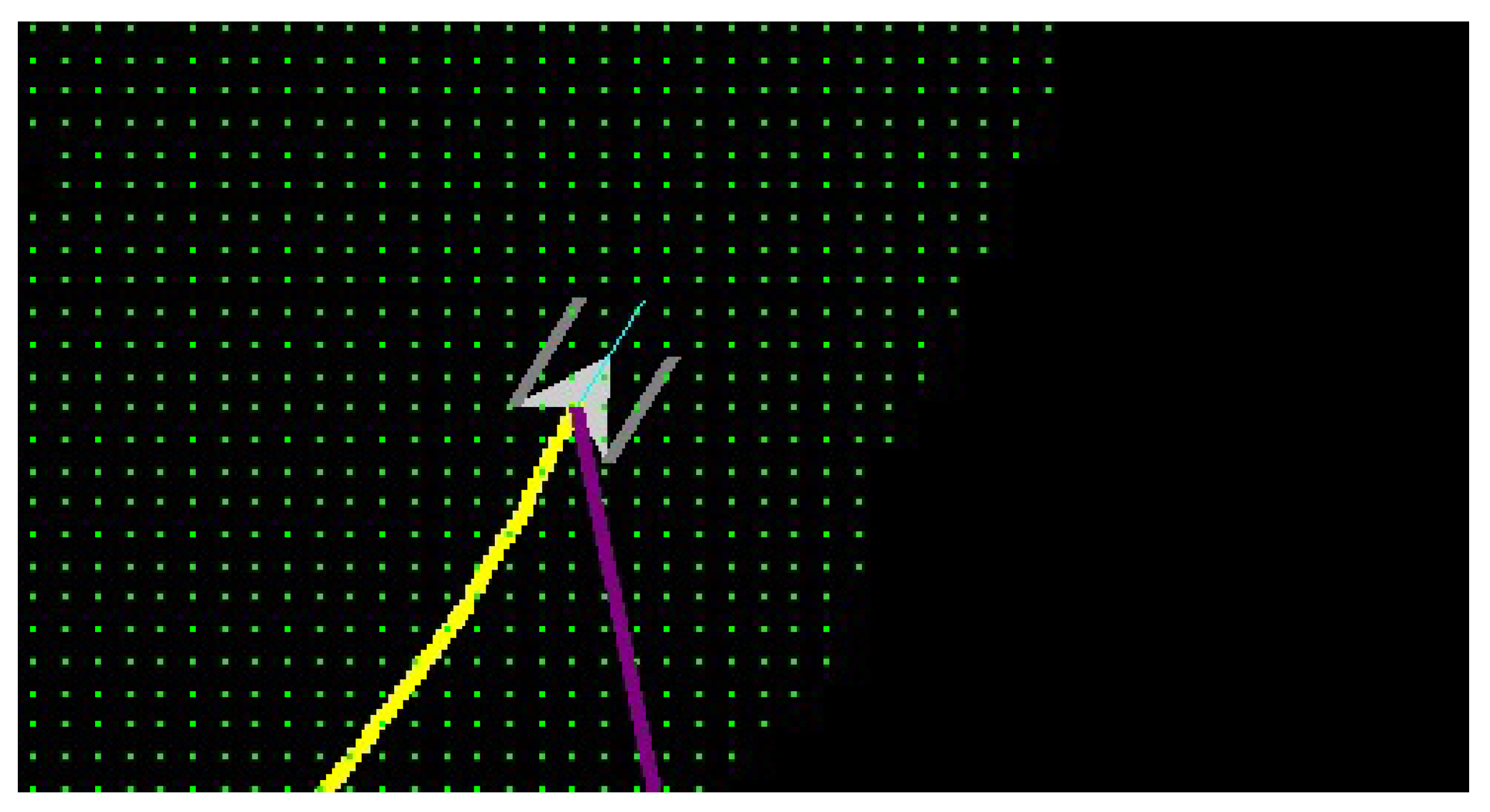
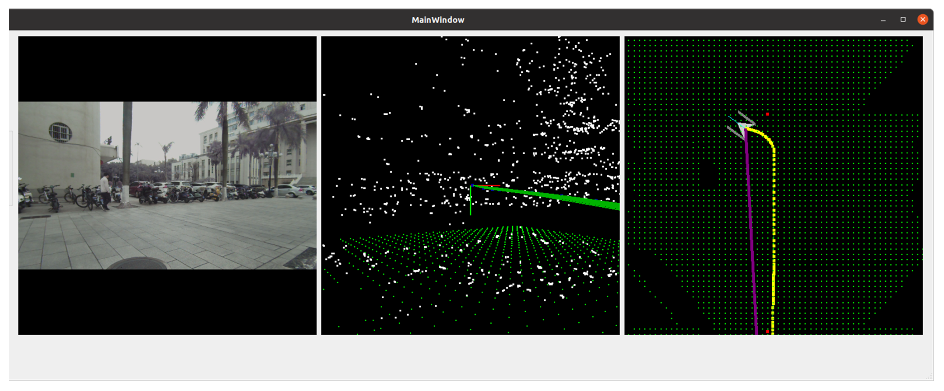
5.2.1. Evaluation of Obstacle Reconstruction in the Scene

The scenes shown in Figure 9a,b feature six square flowerbeds, each approximately 3 m on each side. An occupancy grid map measuring approximately 30 × 30 m was constructed for this scene, with the mapping results presented in Figure 9c. In this map, the green areas represent ground grids, while the black areas indicate the locations of the flowerbeds. Although a few small black areas yielded inaccurate mapping results, the positions of all flowerbeds were successfully reconstructed. However, the shapes of the obstacles could not be accurately reconstructed, as shown in Figure 9e, where the vertices of the flowerbeds do not form perfect squares.

As shown in Figure 9f, we calculated the errors between the positions of each landmark point in the map and their actual positions in the real world. Since the reconstructed obstacles are not perfect squares, some points exhibit larger errors; however, the maximum error is approximately 0.8 m. Most landmark points have errors within 0.4 m, with the minimum error being less than 0.1 m.

To evaluate the effectiveness of our method for reconstructing small-sized obstacles, we examine the mapping results in the scenes shown in Figure 10a,b. The scene contains five circular columns, with the black areas in Figure 10c representing their positions in the map. Four landmark points are selected at the same positions on the circular bases of each column, as illustrated in Figure 10e. Except for the fourth column, which exhibits a relatively large reconstruction error, the remaining columns show satisfactory results. In Figure 10f, we assess the errors of the landmark points along the X-axis and Y-axis. It can be observed that, apart from a few points with significantly larger errors, most errors are concentrated within 0.3 m.

In summary, our method demonstrates superior performance in reconstructing small-sized obstacles. The maps generated using our approach provide a more accurate reconstruction of obstacle positions. However, limitations remain in the reconstruction of obstacle shapes. Nevertheless, since our method is primarily designed to construct navigable grid maps, which often involve obstacle expansion during navigation tasks, the shape reconstruction errors remain within an acceptable range.

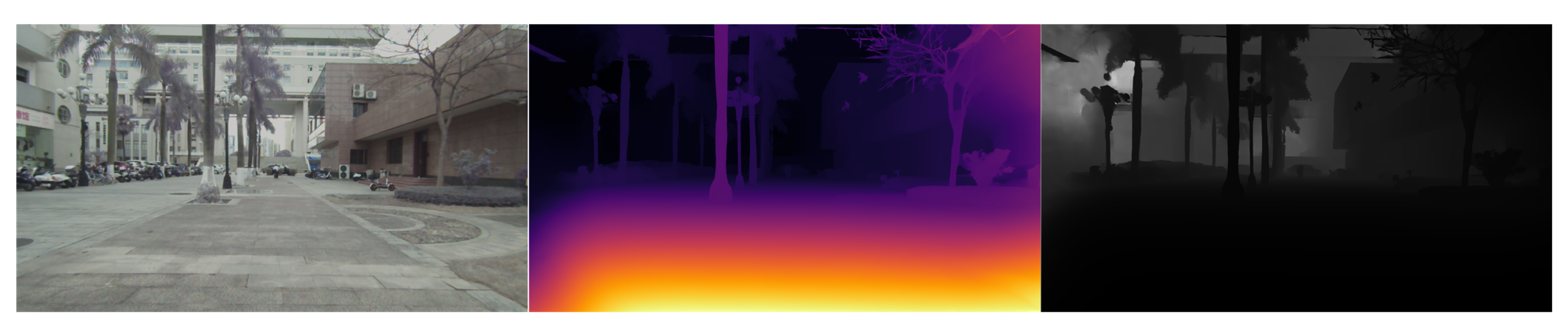
5.2.2. Evaluation of Road Surface Reconstruction in the Scene

As shown in Figure 11a,b, a rectangular road segment, approximately 5 m wide and 130 m long, is selected as the test scene. The green area in Figure 11c represents the road surface in the map. It is evident that, aside from a small section of black error regions in the middle of the road, the road surface reconstruction is generally successful. The red-marked areas in Figure 11c indicate sections where our mapping method incorrectly estimates the road’s width. Our analysis suggests that this error primarily results from the relatively low steps at both ends of the road and sparse grass coverage in these areas. Consequently, the semantic segmentation fails to clearly distinguish between the lawn and the road, leading to an inaccurate reconstruction of this section. The yellow-marked areas in Figure 11c correspond to three bicycles parked in this location, and the black regions in this part are not mapping errors.

To assess the stability of the method, a more complex scene was selected to evaluate the reconstruction of the road surface. Unlike the previous scene, this scenario features a circular road within a park, bordered by stone steps and a lawn. The road width is approximately 3.5 m, with a total length of about 100 m. As shown in Figure 12c, the road surface was successfully reconstructed, with the exception of the areas marked in red. These regions, located at the boundary between the lawn and the road, are where semantic segmentation fails to generate accurate semantic masks, leading to some lawn areas being mistakenly classified as road surface. Landmark points were selected along the inner and outer edges of the road, including the apex, corners, and junctions, as easily identifiable reference points. Figure 12e illustrates the discrepancies between the positions of these landmark points in the map and their actual locations. As shown in Figure 12f, the majority of the landmark point errors are within 0.5 m. The data in

Table 1. The root mean square error (RMSE) of mapping results.

RMSE in Mapping Experiment
Scene	Map Scale (${\mathbf{m}}^{\mathbf{2}}$)	RMSE (m)
		Position x	Position y	Total
Scene 1	900	0.367	0.404	0.386
Scene 2	1200	0.288	0.347	0.319
Scene 3	2100	0.485	0.325	0.413
Scene 4	3000	0.387	0.378	0.382

represent the root mean square error (RMSE) of our mapping method across four distinct scenes.

As shown in Table 1, our method exhibits strong performance across all four scenes, with the RMSE ranging from 0.3 to 0.4 m in each case. Furthermore, during the experiments, our system operates at 30 frames per second, which largely satisfies the requirements for real-time mapping.

6. Discussion

6.1. Performance Comparison

To demonstrate the advantages of our proposed method, we compare it with other approaches in this section. As our primary focus is on applications in real-world scenarios, the comparisons are conducted within such contexts. Dense depth estimation is an effective technique for map construction, as it estimates the depth of obstacles, i.e., the distance between the obstacle and the camera. We compare four depth estimation networks [27,34,35,36], all of which have demonstrated superior performance in recent years.

As shown in Figure 13, since the original output of the stereo matching network is the disparity of the stereo image, we first converted the output disparity map to a depth map using our own camera parameters. To obtain the depth of the target region, we first load a depth image using the OpenCV library. Depth images are usually single-channel images, where each pixel value represents the depth information of the corresponding point in the scene. However, the information in the depth map is often normalized relative values, so we need to extract the original information in the depth matrix based on the corresponding pixel regions in the depth map so that we can get the real depth values. Using OpenCV’s mouse callback mechanism, we implemented a function that allows users to draw any polygonal region on the depth map, generating a binary mask with pixel values of 255 inside the polygon and 0 outside. This enables us to extract the depth values of the corresponding region. Finally, outliers are removed, and the mean value is computed as the final depth of the region. We selected several typical obstacles in the real world and measured their actual distances. Subsequently, we applied the four aforementioned stereo matching algorithms for depth estimation and computed their root mean square errors, as presented in Table 2.

Table 2. The comparison of the root mean square error (RMSE).

Performance Comparison Based on RMSE
Method	RMSE (m)
	Scene 1	Scene 2	Scene 3	Scene 4	Scene 5	Total
CroCo-Stereo [34]	0.285	0.314	0.296	0.311	0.330	0.307
ACVNet [35]	0.455	0.398	0.427	0.379	0.443	0.420
PCVNet [36]	0.650	0.673	0.612	0.675	0.710	0.637
CREStereo [27]	0.472	0.411	0.521	0.439	0.490	0.467

Table 2. The comparison of the root mean square error (RMSE).

Performance Comparison Based on RMSE
Method	RMSE (m)
	Scene 1	Scene 2	Scene 3	Scene 4	Scene 5	Total
CroCo-Stereo [34]	0.285	0.314	0.296	0.311	0.330	0.307
ACVNet [35]	0.455	0.398	0.427	0.379	0.443	0.420
PCVNet [36]	0.650	0.673	0.612	0.675	0.710	0.637
CREStereo [27]	0.472	0.411	0.521	0.439	0.490	0.467

Comparison of Table 1 and Table 2 shows that our algorithm is competitive compared with other methods. Among them, CroCo-Stereo [34] performs better than our algorithm; however, accuracy is not the only evaluation metrics—the efficiency and speed also needs to be considered. Therefore, we also compared the Graphic Processing Unit (GPU) memory usage and the time required to process one frame of the input image on the RTX 3070.

As can be seen from

Table 3. The comparison of efficiency and speed.

Method	CroCo-Stereo	ACVNet	PCVNet	CREStereo	Ours (FCN)
Time (ms)	2151	693	101	1361	96
GPU memory (GB)	2.85	3.2	1.21	1.26	1.1

, though CroCo-Stereo performs excellently, it consumes much more resources and time than ours to process one frame. Thanks to the high efficiency of FCN, our method achieves high performance and low consumption and most likely to achieve real-time mapping.

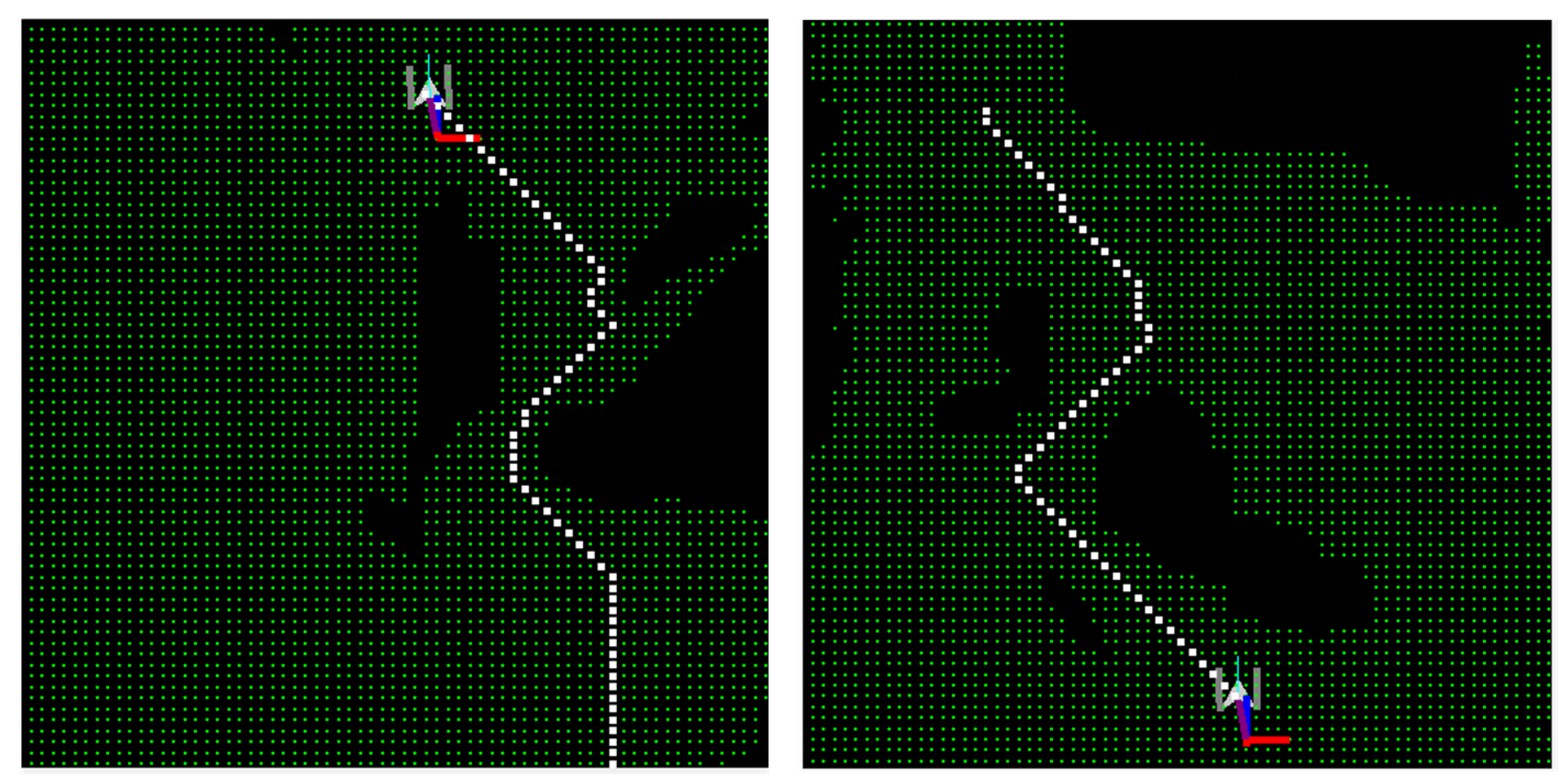
6.2. Example Application

As mentioned earlier, the sparse feature maps generated by SLAM systems are unsuitable for path planning, and we propose a method to construct navigation maps capable of real-time operation in real-world environments. To highlight our contribution and showcase its practical potential, we present a demonstration application. We implement an A* [37] path-planning algorithm as an example of autonomous navigation for a self-built AGV. A detailed discussion of the vehicle’s motion control algorithm is beyond the scope of this paper, and here, we focus on its path planning and navigation using the constructed map.

Figure 14 presents the interactive interface of the navigation system, comprising three windows. From left to right, these windows display the vehicle’s front view, sparse map points, and an occupancy grid map. The map window displays the vehicle’s real-time position and orientation, along with yellow dots indicating its movement trajectory. Additionally, users can interact with the map window by zooming in and out using the mouse scroll wheel. Each green point on the map is clickable. Users can double-click the right mouse button to select a starting point and an intermediate point. A path is then planned based on these two points, as illustrated in Figure 15. The white trajectory represents the output of the path-planning algorithm. Subsequently, the vehicle follows the planned trajectory to reach its destination.

6.3. Limitations and Future Work

While our system demonstrates good performance and significant application potential, certain limitations remain. For instance, our method is still limited by inaccurate semantic masks. Future work will focus on selecting a CNN tailored for this task and optimizing the data association process to reduce the impact of inaccurate semantic masks. Furthermore, the system is not designed to handle dynamic objects, as it primarily focuses on navigation map construction for static environments. Although dynamic feature point removal and path planning for dynamic objects represent two distinct research areas, incorporating these capabilities into our system would enhance its performance in real-world applications; thus, we will prioritize research in these areas. Additionally, since the mapping system and motor control of our AGV are self-developed, the navigation system is relatively straightforward to debug within our framework. However, external users may face challenges in utilizing our program. To address this, we plan to develop a Robot Operating System (ROS) version of the system, which will provide a more versatile framework, facilitating easier integration and deployment.

7. Conclusions

This paper presents a multi-submap fusion mapping approach utilizing semantic ground fitting to construct an occupancy grid map for robot navigation within a global coordinate system. The key contributions of this work are as follows. First, the method simplifies environmental reconstruction by focusing exclusively on the road surface and obstacles, constructing a lightweight navigation map. Additionally, we introduce a novel 3 × 3 grid-based submap management strategy to enable real-time map storage and retrieval, balancing mapping accuracy and computational efficiency. We addressed the issue that sparse point cloud maps generated by visual SLAM algorithms cannot be used for navigation and that real-time mapping is not feasible using dense depth estimation. We evaluated our method in real-world scenarios and presented a practical application in which the constructed map is utilized for AGV navigation. Experimental results confirm that the proposed method efficiently constructs an occupancy grid map for outdoor environments while reducing computational overhead, achieving high accuracy across areas of up to 3000 square meters. While our method demonstrates significant application potential, it has some limitations, including occasional inaccuracies in semantic segmentation and an inability to handle dynamic objects. In future work, we will train the model on our own dataset tailored for specific scenarios to enhance semantic segmentation performance, as well as incorporate dynamic feature point removal and local path planning. Additionally, to improve system integration and portability, we will develop an ROS version of the system.

References

1. Viswanathan, D.G. Features from accelerated segment test (fast). In Proceedings of the 10th Workshop on Image Analysis for Multimedia Interactive Services, London, UK, 6–8 May 2009; pp. 6–8. [Google Scholar]
2. Calonder, M.; Lepetit, V.; Strecha, C.; Fua, P. Brief: Binary robust independent elementary features. In Proceedings of the Computer Vision–ECCV 2010: 11th European Conference on Computer Vision, Heraklion, Greece, 5–11 September 2010; Springer: Cham, Switzeraland, 2010; pp. 778–792. [Google Scholar]
3. Mur-Artal, R.; Montiel, J.M.M.; Tardos, J.D. ORB-SLAM: A versatile and accurate monocular SLAM system. IEEE Trans. Robot. 2015, 31, 1147–1163. [Google Scholar]
4. Mur-Artal, R.; Tardós, J.D. Orb-slam2: An open-source slam system for monocular, stereo, and rgb-d cameras. IEEE Trans. Robot. 2017, 33, 1255–1262. [Google Scholar] [CrossRef]
5. Campos, C.; Elvira, R.; Rodríguez, J.J.G.; Montiel, J.M.; Tardós, J.D. Orb-slam3: An accurate open-source library for visual, visual–inertial, and multimap slam. IEEE Trans. Robot. 2021, 37, 1874–1890. [Google Scholar] [CrossRef]
6. Cheng, J.; Zhang, L.; Chen, Q.; Hu, X.; Cai, J. A review of visual SLAM methods for autonomous driving vehicles. Eng. Appl. Artif. Intell. 2022, 114, 104992. [Google Scholar] [CrossRef]
7. Newcombe, R.A.; Izadi, S.; Hilliges, O.; Molyneaux, D.; Kim, D.; Davison, A.J.; Kohi, P.; Shotton, J.; Hodges, S.; Fitzgibbon, A. Kinectfusion: Real-time dense surface mapping and tracking. In Proceedings of the 2011 10th IEEE International Symposium on Mixed and Augmented Reality, Basel, Switzeraland, 26–29 October 2011; pp. 127–136. [Google Scholar]
8. McCormac, J.; Handa, A.; Davison, A.; Leutenegger, S. Semanticfusion: Dense 3d semantic mapping with convolutional neural networks. In Proceedings of the 2017 IEEE International Conference on Robotics and Automation (ICRA), Singapore, 29 May–3 June 2017; pp. 4628–4635. [Google Scholar]
9. Runz, M.; Buffier, M.; Agapito, L. Maskfusion: Real-time recognition, tracking and reconstruction of multiple moving objects. In Proceedings of the 2018 IEEE International Symposium on Mixed and Augmented Reality (ISMAR), Munich, Germany, 16–20 October 2018; pp. 10–20. [Google Scholar]
10. Tosi, F.; Bartolomei, L.; Poggi, M. A survey on deep stereo matching in the twenties. Int. J. Comput. Vis. 2025, 1–32. [Google Scholar] [CrossRef]
11. Li, Y.; Zhao, H.; Qi, X.; Wang, L.; Li, Z.; Sun, J.; Jia, J. Fully convolutional networks for panoptic segmentation. In Proceedings of the IEEE/CVF Conference on Computer Vision and Pattern Recognition, Nashville, TN, USA, 20–25 June 2021; pp. 214–223. [Google Scholar]
12. Ming, Y.; Meng, X.; Fan, C.; Yu, H. Deep learning for monocular depth estimation: A review. Neurocomputing 2021, 438, 14–33. [Google Scholar] [CrossRef]
13. Liu, C.W.; Wang, H.; Guo, S.; Bocus, M.J.; Chen, Q.; Fan, R. Stereo matching: Fundamentals, state-of-the-art, and existing challenges. In Autonomous Driving Perception: Fundamentals and Applications; Springer: Berlin/Heidelberg, Germany, 2023; pp. 63–100. [Google Scholar]
14. Mertan, A.; Duff, D.J.; Unal, G. Single image depth estimation: An overview. Digit. Signal Process. 2022, 123, 103441. [Google Scholar]
15. Tsardoulias, E.G.; Iliakopoulou, A.; Kargakos, A.; Petrou, L. A review of global path planning methods for occupancy grid maps regardless of obstacle density. J. Intell. Robot. Syst. 2016, 84, 829–858. [Google Scholar] [CrossRef]
16. Lowe, G. Sift-the scale invariant feature transform. Int. J. 2004, 2, 2. [Google Scholar]
17. Bay, H.; Tuytelaars, T.; Van Gool, L. Surf: Speeded up robust features. In Proceedings of the Computer Vision–ECCV 2006: 9th European Conference on Computer Vision, Graz, Austria, 7–13 May 2006; Proceedings, Part I 9; Springer: Cham, Switzerland, 2006; pp. 404–417. [Google Scholar]
18. Rublee, E.; Rabaud, V.; Konolige, K.; Bradski, G. ORB: An efficient alternative to SIFT or SURF. In Proceedings of the 2011 International Conference on Computer Vision, Barcelona, Spain, 6–13 November 2011; pp. 2564–2571. [Google Scholar]
19. Gálvez-López, D.; Tardos, J.D. Bags of binary words for fast place recognition in image sequences. IEEE Trans. Robot. 2012, 28, 1188–1197. [Google Scholar] [CrossRef]
20. Cao, S.; Lu, X.; Shen, S. GVINS: Tightly coupled GNSS–visual–inertial fusion for smooth and consistent state estimation. IEEE Trans. Robot. 2022, 38, 2004–2021. [Google Scholar]
21. Qin, T.; Li, P.; Shen, S. Vins-mono: A robust and versatile monocular visual-inertial state estimator. IEEE Trans. Robot. 2018, 34, 1004–1020. [Google Scholar] [CrossRef]
22. Xiong, L.; Kang, R.; Zhao, J.; Zhang, P.; Xu, M.; Ju, R.; Ye, C.; Feng, T. G-VIDO: A vehicle dynamics and intermittent GNSS-aided visual-inertial state estimator for autonomous driving. IEEE Trans. Intell. Transp. Syst. 2021, 23, 11845–11861. [Google Scholar] [CrossRef]
23. Liu, J.; Gao, W.; Hu, Z. Optimization-based visual-inertial SLAM tightly coupled with raw GNSS measurements. In Proceedings of the 2021 IEEE International Conference on Robotics and Automation (ICRA), Xi’an, China, 30 May–5 June 2021; pp. 11612–11618. [Google Scholar]
24. Zhu, J.; Zhou, H.; Wang, Z.; Yang, S. Improved Multi-sensor Fusion Positioning System Based on GNSS/LiDAR/Vision/IMU with Semi-tightly Coupling and Graph Optimization in GNSS Challenging Environments. IEEE Access 2023, 11, 95711–95723. [Google Scholar]
25. Xu, L.; Feng, C.; Kamat, V.R.; Menassa, C.C. An occupancy grid mapping enhanced visual SLAM for real-time locating applications in indoor GPS-denied environments. Autom. Constr. 2019, 104, 230–245. [Google Scholar]
26. Chang, Q.; Li, X.; Xu, X.; Liu, X.; Li, Y.; Miyazaki, J. StereoVAE: A lightweight stereo-matching system using embedded GPUs. In Proceedings of the 2023 IEEE International Conference on Robotics and Automation (ICRA), London, UK, 29 May–2 June 2023; pp. 1982–1988. [Google Scholar]
27. Li, J.; Wang, P.; Xiong, P.; Cai, T.; Yan, Z.; Yang, L.; Liu, J.; Fan, H.; Liu, S. Practical stereo matching via cascaded recurrent network with adaptive correlation. In Proceedings of the IEEE/CVF Conference on Computer Vision and Pattern Recognition, New Orleans, LA, USA, 18–24 June 2022; pp. 16263–16272. [Google Scholar]
28. Xu, G.; Wang, X.; Ding, X.; Yang, X. Iterative geometry encoding volume for stereo matching. In Proceedings of the IEEE/CVF Conference on Computer Vision and Pattern Recognition, Vancouver, BC, Canada, 17–24 June 2023; pp. 21919–21928. [Google Scholar]
29. Wu, Z.; Zhu, H.; He, L.; Zhao, Q.; Shi, J.; Wu, W. Real-time stereo matching with high accuracy via Spatial Attention-Guided Upsampling. Appl. Intell. 2023, 53, 24253–24274. [Google Scholar]
30. Kümmerle, R.; Grisetti, G.; Strasdat, H.; Konolige, K.; Burgard, W. g 2 o: A general framework for graph optimization. In Proceedings of the 2011 IEEE international Conference on Robotics and Automation, Shanghai, China, 9–13 May 2011; pp. 3607–3613. [Google Scholar]
31. Tsai, R. A versatile camera calibration technique for high-accuracy 3D machine vision metrology using off-the-shelf TV cameras and lenses. IEEE J. Robot. Autom. 1987, 3, 323–344. [Google Scholar] [CrossRef]
32. Jiang, Z.; Liu, J.; Wang, F.; Bei, J.; Zhai, X. Research on construction Theory of Global cGcs2000 coordinate Frame. Geomat. Inf. Sci. Wuhan Univ. 2018, 43, 167–174. [Google Scholar]
33. Liang, Y.; Li, Y.; Yu, Y.; Zheng, L. Integrated lateral control for 4WID/4WIS vehicle in high-speed condition considering the magnitude of steering. Veh. Syst. Dyn. 2020, 58, 1711–1735. [Google Scholar]
34. Weinzaepfel, P.; Lucas, T.; Leroy, V.; Cabon, Y.; Arora, V.; Brégier, R.; Csurka, G.; Antsfeld, L.; Chidlovskii, B.; Revaud, J. Croco v2: Improved cross-view completion pre-training for stereo matching and optical flow. In Proceedings of the IEEE/CVF International Conference on Computer Vision, Paris, France, 2–6 October 2023; pp. 17969–17980. [Google Scholar]
35. Xu, G.; Cheng, J.; Guo, P.; Yang, X. Attention concatenation volume for accurate and efficient stereo matching. In Proceedings of the IEEE/CVF Conference on Computer Vision and Pattern Recognition, New Orleans, LA, USA, 18–24 June 2022; pp. 12981–12990. [Google Scholar]
36. Zeng, J.; Yao, C.; Yu, L.; Wu, Y.; Jia, Y. Parameterized cost volume for stereo matching. In Proceedings of the IEEE/CVF International Conference on Computer Vision, Paris, France, 2–6 October 2023; pp. 18347–18357. [Google Scholar]
37. Zhang, W.; Wang, N.; Wu, W. A hybrid path planning algorithm considering AUV dynamic constraints based on improved A* algorithm and APF algorithm. Ocean Eng. 2023, 285, 115333. [Google Scholar] [CrossRef]
Figure 1. Framework of the proposed method.
Applsci 15 03725 g001
Figure 2. Occupancy grid map construction algorithm flowchart.
Applsci 15 03725 g002
Figure 3. The projection process among different coordinate systems.
Applsci 15 03725 g003
Figure 4. The switching process of the three maps during map updates.
Applsci 15 03725 g004
Figure 5. Self-constructed experimental platform.
Applsci 15 03725 g005
Figure 6. List of experimental equipment. SinoGNSS RTK: Shanghai SinoGNSS Navigation Technology Co., Ltd. (Shanghai, China). MYNTAI Stereo Camera: Shenzhen MYNTAI Technology Co., Ltd. (Shenzhen, China). Lenovo Legion Laptop: Lenovo Group Ltd. (Beijing, China).
Applsci 15 03725 g006
Figure 7. Experimental scenarios in the real world. (a,b) are used to evaluate the reconstruction of obstacles, (c,d) are primarily used to assess the reconstruction of the road surface.
Applsci 15 03725 g007
Figure 8. The OGM visualization format proposed in this paper.
Applsci 15 03725 g008
Figure 9. Mapping results for Scene 1. (a,b) The real environment photographs, (c) the visualization of the OGM mapping results, (d) the ground truth of landmark points, (e) the comparison between the sampled points and the ground truth, and (f) the errors in the x-axis and y-axis for mapping results.
Applsci 15 03725 g009
Figure 10. Mapping results for Scene 2. (a,b) The real environment photographs, (c) the visualization of the OGM mapping results, (d) the ground truth of landmark points, (e) the comparison between the sampled points and the ground truth, and (f) the errors in the x-axis and y-axis for mapping results.
Applsci 15 03725 g010
Figure 11. Mapping results for Scene 3. (a,b) The real environment photographs, (c) the visualization of the OGM mapping results, (d) the ground truth of landmark points, (e) the comparison between the sampled points and the ground truth, and (f) the errors in the x-axis and y-axis for mapping results.
Applsci 15 03725 g011
Figure 12. Mapping results for Scene 4. (a,b) The real environment photographs, (c) the visualization of the OGM mapping results, (d) the ground truth of landmark points, (e) the comparison between the sampled points and the ground truth, and (f) the errors in the x-axis and y-axis for mapping results.
Applsci 15 03725 g012
Figure 13. Obtaining depth information after converting the original image to a depth map.
Applsci 15 03725 g013
Figure 14. Visual interactive interface for navigation systems.
Applsci 15 03725 g014
Figure 15. Route planning using constructed maps. The green area represents the navigable region, the black area represents the non-navigable region, and the white dots indicate the planned route.
Applsci 15 03725 g015