Abstract
In the field of mobile robot path planning, traditional genetic algorithms face issues such as slow convergence, lack of dynamic adaptability, and uncertain mutation directionality. To address these issues, a dichotomy-based multi-step method was used during the population initialization phase to enhance both the quality and diversity of the population. The selection strategy was improved for tournament selection, which reduces the monopolistic dominance of exceptional individuals and preserves population diversity through multiple rounds of grouping competitions. The crossover strategy adopted an adaptive crossover point number, with parents chosen based on a dynamic threshold. The mutation strategy combines a two-layer encoding approach: the first layer uses random mutations to enhance diversity, while the second layer performs goal-oriented mutations, with the selection probability of each layer dynamically adjusted during iterations. Bezier curve optimization of the optimal path was conducted. Experimental results show that the improved genetic algorithm demonstrates significant advantages in terms of path length, smoothness, iteration speed, and computational efficiency.
1. Introduction
With the rapid development of mobile robotics technology, path planning, as one of the core issues in mobile-robot autonomous navigation, has garnered widespread attention [1]. The goal of path planning is to find an optimal path from the starting point to the destination within a given environment while avoiding obstacles [2]. Its applications span across various domains, including material handling in industrial production, intelligent transportation in logistics, robot guidance in the service industry [3], and unmanned combat in military fields, demonstrating its broad potential for application [4].
Currently, mobile-robot path planning algorithms can be classified into traditional path planning algorithms, sampling-based path planning algorithms, and intelligent bionic algorithms [5]. Traditional path planning algorithms include the A* algorithm [6], the Dijkstra algorithm [7], the D* algorithm [8], and the artificial potential field method [9], while sampling-based path planning algorithms include the PRM algorithm [10] and the RRT algorithm [11]. Intelligent bionic path planning algorithms include neural network algorithms [12], particle swarm optimization [13], ant colony optimization [14], and genetic algorithms [15].
Genetic algorithms, as global optimization algorithms based on biological evolution principles, have gradually become effective tools for solving complex path planning problems due to their strong global search capabilities and robustness [16]. However, the application of traditional genetic algorithms in robot path planning still has many shortcomings [17]. On one hand, the initial population quality is low, leading to slow convergence [18]; on the other hand, traditional selection strategies may allow exceptional individuals to dominate the population, causing the algorithm to fall into local optima and reducing population diversity and exploration ability [19]. Furthermore, the crossover operation lacks sufficient local search capabilities and may disrupt well-formed gene combinations, while the mutation operation lacks directionality [20], potentially damaging high-fitness individuals and making path quality difficult to control.
To address these issues, various improvement methods have been proposed in the literature. For instance, in reference [21], a population initialization strategy based on linear ranking was proposed for the CBPRM algorithm. By assigning scores to environmental cells based on their distance to the target, linear ranking replaces the roulette selection method to determine cell selection probabilities. Starting from the initial point, the strategy excludes cells containing obstacles and sequentially selects available cells to construct a feasible path to the target point. If no available cells are found before reaching the target, path construction terminates. In reference [22], two special lists are used to select parents: one list contains high-fitness paths chosen by elite selection, and the other contains paths with different fitness values. This approach improves the quality of offspring while allowing low-fitness parents to explore the search space. During offspring generation, multiple potential offspring are created based on feasible crossover points, and the two paths with the highest fitness are selected after sorting. In traditional mutation operations, only one node typically has the chance to mutate. Reference [23] designs a dual AGV collaborative safety steering radius, integrating multiple factors into the global path planning algorithm to prevent steering collisions and balance the planning efficiency with map utilization. It introduces the starting- and ending-point posture information and initializes the path based on safety steering rules, thoroughly considering the potential for steering collisions between the dual AGVs at the start and end points, thus generating a safer initial path. Reference [24] introduces a Markov chain that can predict future states based on current ones. The path is represented as a grid number, and during mutation operations, the initial number sequence is randomly truncated. From the truncation point, subsequent grid numbers are selected based on state transition probabilities to form a new sequence. Rules are set to avoid the robot from going back or remaining stationary, guiding individual changes to find better paths. Reference [25] introduces operators for loop removal, insertion–deletion, and optimization, which are used for deleting loops, adjusting nodes, and shrinking paths.
Although these improvements have achieved significant results in some respects, they also increase the complexity of the algorithm, extend computation time, and impose higher requirements on hardware. At the same time, these improvement directions are relatively narrow and make it difficult to achieve global optimization. Therefore, this paper proposes a series of improvements, including a dichotomy-based multi-step method for population initialization, a tournament selection strategy, an adaptive crossover strategy, a two-layer encoding mutation strategy and the Bezier curve optimization of the optimal path. These improvements not only enhance the quality and diversity of the population but also strengthen the algorithm’s adaptability and search efficiency at different stages. The goal is to provide a more efficient and robust solution for robot path planning.
2. Environment Mapping
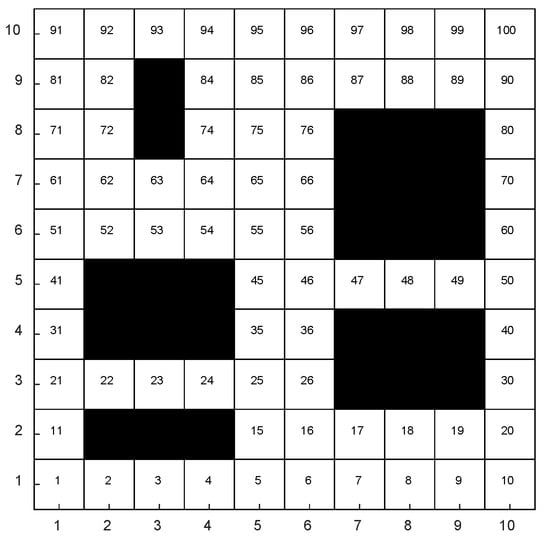
In the application of path planning, the grid method is a commonly used modeling approach. This method discretizes the continuous planning space into a series of equally sized grids (grid cells), simplifying complex environmental information into a simple one-dimensional array format. Each grid cell corresponds to a region in the actual environment, and the specific attributes of that region are represented by the state of the grid map. To ensure the effectiveness of path planning, the size of each grid cell is typically determined based on the robot’s own dimensions, the size of obstacles, and the characteristics of the working environment, in order to be applicable to non-grid environments.
In the grid map, black grid cells represent obstacles, while white grid cells indicate the feasible free-movement areas. Additionally, to prevent the robot from exceeding the boundaries of the map during the path planning process, it is typically assumed that the perimeter of the grid map is completely surrounded by obstacles, thus forming a safe boundary constraint, as shown in Figure 1.
Figure 1.
Grid matrix diagram.
The coordinates (x, y) of each grid cell can be uniquely mapped to a grid index, and the relationship between the grid index and coordinates is given by the following formula:
where floor is the floor function, num is the grid index, row is the number of columns in the grid map, and G(x, y) is the matrix of feasible grid cells.
3. Improved Genetic Algorithm
3.1. Population Initialization
The quality of the initial population in a genetic algorithm is crucial to the solution’s outcome. The initial population generated by traditional genetic algorithms tends to be of poor quality, which in turn affects the convergence speed of the algorithm. In this study, a binary search method combined with a multi-step length approach is used for population initialization. This not only significantly enhances the diversity of the population but also effectively improves its quality.
3.1.1. Dichotomy Method
The core idea of the dichotomy method is to recursively find the midpoint between two grid cells. It is primarily implemented using two approaches: the row-based method and the column-based method.
The processing flow of the base–row system and base–column system adjusts the judgment sequence according to the base dichotomy type: the base–row system checks if the vertical coordinate difference |Y − y| is greater than one, while the base–column system checks if the horizontal coordinate difference |X − x| is greater than one. When the difference exceeds the threshold, a bisection operation is performed: the coordinate difference is divided by two and randomly rounded (either rounded up or down), with the same calculation rule applied to both horizontal and vertical coordinates. After generating the midpoint, if an obstacle is encountered, the movement direction is chosen based on the base direction type: the base–row system uses horizontal (left/right) displacement, while the base–column system uses vertical (up/down) displacement, continuing to move within the current row or column to find a feasible grid. If no valid path is found after the displacement, the algorithm is terminated, indicating that no path exists between the start and end points in the current map. The base–row system and base–column system each ensure that there is one grid per row or column. By evenly splitting the population into two base direction modes and introducing the random rounding of the half-coordinate difference and obstacle-avoiding random-direction selection mechanisms, the initial population diversity is significantly enhanced, thereby optimizing the global performance of the algorithm.
After applying the dichotomy method to generate intermediate points between the start and end points, the path is divided into two segments. For each segment, the search for intermediate points continues, further subdividing the path until adjacent rows or columns can no longer be divided. The final path generated will consist of multiple nodes that are evenly distributed.
3.1.2. The Multi-Step Method
Traditional path planning algorithms typically use the grid center points as a standard, where the path travels from the starting point through several center points to the destination. This method is simple and effective, but it has significant drawbacks: the path is constrained by the grid centers, often resulting in a stair-step or polyline shape, lacking smoothness and a natural feel. Additionally, in complex obstacle environments, excessive reliance on grid centers may prevent the discovery of an effective path, resulting in a lack of flexibility and robustness.
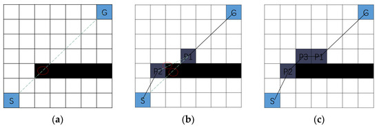
Since the Bresenham algorithm does not require floating-point operations, it conserves hardware resources, as its integer arithmetic avoids the high cost and inefficiency associated with complex floating-point calculations. Therefore, an improved multi-step method based on the Bresenham algorithm is proposed, which eliminates the constraint of grid centers. This method directly detects the linear connectivity between two points. If the two points are directly connected, a straight-line path is generated; if obstructed by an obstacle, intermediate nodes are dynamically inserted, prioritizing the midpoint or nearby free grid cells for adjustment, to ensure the connectivity and feasibility of the path. As shown in Figure 2, the green dashed line represents the determination of whether the straight line passes through an obstacle based on the Bresenham algorithm; the black solid line represents the feasible path segment; P1, P2, and P3 are insertion points; and the red circles indicate locations where the straight line intersects obstacles.
Figure 2.
Multi-step principle diagram. (a) step1; (b) step2; (c) step3.
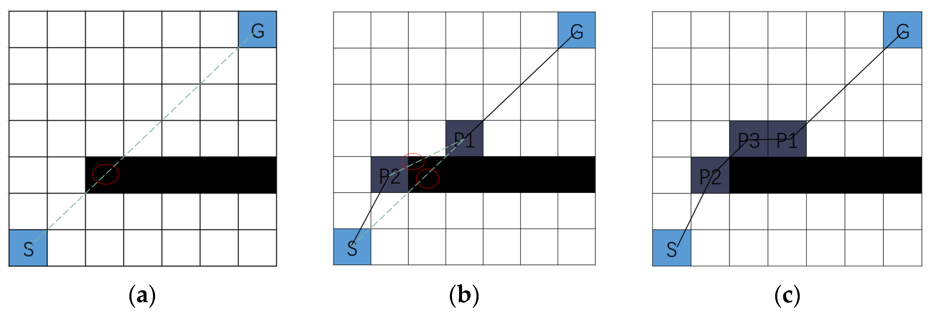
However, the traditional Bresenham algorithm can only directly identify the dark-blue grid cells shown in Figure 3, while the light-colored grid cells will be missed. To address this issue, this paper improves the Bresenham algorithm by adding a detection mechanism for light-colored grid cells, enabling it to identify all the grid cells that the line passes through. Method for detecting light-colored grid cells: taking the line with slope and the grid cells A and B from Figure 3 as an example, when the Bresenham algorithm computes the change in the y-coordinate of grid cell B, compare with . If > , the line passes through the cell above A; if = , the line passes through only both grid cells A and B; if < , the line passes through the cell below B. This is shown in Figure 3.
Figure 3.
The improved Bresenham algorithm detects all the grid cells a straight line passes through.
The specific steps of the improved Bresenham algorithm for detecting the grid cells a straight line passes through are as follows:
Step 1: Input the coordinates of the two endpoints, (,) and (,), and initialize an empty array [X, Y].
Step 2: Calculate dx = || and ||. If dx < dy, swap the x and y coordinates to ensure stepping along the y-axis. If > , swap the start and end coordinates to ensure traversal from left to right.
Step 3: Traverse the x coordinates from left to right. Each time x moves one step forward, accumulate the error. If the error exceeds the threshold, update the y coordinate and add the updated coordinates (x, y) to the [X, Y] set (if dx < dy, swap the coordinates before adding to [X, Y]). Each time the y coordinate is updated, check for any missing grid cells. If there are any, they should be supplemented promptly, and the supplemented grid cells should also be added to [X, Y] (similarly, when dx < dy, swap the coordinates before adding to [X, Y]).
Step 4: Return the array [X, Y], which contains the coordinates of all grid cells on the path.
The improved Bresenham algorithm is shown in Algorithm 1.
| Algorithm 1 Improved Bresenham algorithm |
| 1: Input: Coordinates of two endpoints (x1,y1) and (x2,y2) |
| 2: Output: Coordinate set [X, Y] |
| 3: Initialize parameters |
| 4: dx←|x2 − x1|; dy←|y2 − y1|; steep←(dy > dx); |
| 5: if steep |
| 6: Swap x and y coordinates for both endpoints; |
| 7: end |
| 8: if x1 > x2 |
| 9: Swap both coordinates of start and end points; |
| 10: end |
| 11: error ← 0; y←y1; [X, Y]←[∅, ∅]; k←dy/dx; |
| 12: step ← sign(y2 − y1); |
| 13: for x = x1: x2 |
| 14: [a, b] ← steep ? [y, x] : [x, y]; |
| 15: X ← [X, a]; Y ← [Y, b]; |
| 16: error = error + dy; |
| 17: if 2 × error >= dx |
| 18: ideal ← (x + 0.5 − x1) × k + y1; |
| 19: diff ← ideal − (y + 0.5); |
| 20: if diff > 0 |
| 21: [a_add, b_add] ← steep ? [y + 1, x] : [x, y + 1]; |
| 22: X ← [X, a_add]; Y ← [Y, b_add]; |
| 23: elseif diff < 0 |
| 24: [a_add, b_add] ← steep ? [y, x + 1] : [x + 1, y]; |
| 25: X ← [X, a_add]; Y ← [Y, b_add]; |
| 26: end |
| 27: y ← y + step; error ← error − dx; |
| 28: end |
| 29: end |
3.1.3. Generating Initial Population Individuals
Since the path generated by the dichotomy method is discontinuous, a multi-step approach is required to connect adjacent grid cells, thereby generating a continuous path. This ensures the coherence and feasibility of each individual in the path planning process.
3.2. Improved Selection Strategy
The traditional selection method in genetic algorithms is roulette wheel selection, where the selection probability is associated with the individual’s fitness. When a few exceptional individuals dominate the population, they may be selected frequently during the selection process, causing the next generation to be quickly dominated by these individuals. As a result, the population becomes homogeneous, losing competitiveness and exploration ability, potentially falling into a local optimum. The selection probability can be expressed as
where is the selection probability of the i-th individual in the roulette wheel selection method, is the fitness value of the i-th individual in the population, and is the population size, where .
To address this issue, an improved tournament selection method is proposed. This method reduces the absolute dominance of exceptional individuals by using multiple rounds of group competitions, introducing more randomness and competitive layers. As a result, individuals with lower fitness values may also be selected, effectively preserving population diversity and avoiding convergence to a local optimum. The specific steps are as follows:
Step 1: Set the population size to n (where n is a multiple of 32).
Step 2: Randomly divide the population into G groups, where . Each group undergoes a layered competition, including preliminary rounds, semifinals, and finals. The competition selects the four individuals with the highest fitness in each group. In each round of the tournament, a total of 4G individuals are selected.
Step 3: Repeat Step 2 for eight rounds of the tournament. In the end, a total of n individuals are selected.
The improved tournament selection is shown in Algorithm 2.
| Algorithm 2 Improved Tournament Selection |
| 1: Input: Population P (size N); Fitness values F (length N) |
| 2: Output: selected_pop |
| 3: Initialize parameters |
| 4: Group size G ← 32; Groups per tournament K ← 4; Winners per group W ← 4; |
| 5: selected_pop ← ∅; |
| 6: T ← N/(K × W); |
| 7: for t = 1 : T |
| 8: I ← randperm(NP); |
| 9: Split I into K groups G1,…,G_K (each size G); |
| 10: for i = 1: K |
| 11: S1 ← []; S2 ← [] ; W_i← [] ; |
| 12: for j: 2:G_K |
| 13: (ind1, ind2) ← (G_i[j], G_i[j + 1]); |
| 14: S1 ← S1 ∪ [F[ind1] > F[ind2] ? ind1 : ind2]; |
| 15: end |
| 16: for j: 2: length(S1) |
| 17: S2 ← S2 ∪ [F[ind1] > F[ind2] ? ind1 : ind2]; |
| 18: end |
| 19: for j: 2: length(S2) |
| 20: (ind1, ind2) ← (S2[j], S2[j + 1]); |
| 21: W_i ← W_i ∪ [F[ind1] > F[ind2] ? ind1 : ind2]; |
| 22: end |
| 23: selected_pop ←selected_pop ∪ W_i; |
| 24: end |
| 25: end |
3.3. Improved Crossover Strategy
In traditional genetic algorithms, crossover operations typically involve a fixed number of crossover points and randomly selected parents. This fixed crossover point approach lacks flexibility. In the early stages of the algorithm, strong exploration capabilities are usually needed to broaden the search space, whereas in the later stages, more refined exploitation capabilities are required to fine-tune the solution. Fixed crossover points do not meet these dynamic needs. Additionally, the completely random selection of parents may lead to the crossover of individuals with significantly different fitness levels, which can dilute or even destroy superior genes with superior ones, thereby reducing the quality of new individuals and hindering the algorithm’s evolution toward the optimal solution. To address these issues, this paper proposes adaptive crossover point numbers and dynamic threshold selection.
The adaptive number of crossover points is determined by the following formula:
where P is the number of crossover points; floor is the floor function (which rounds down to the nearest integer), is the maximum number of crossover points, t is the current iteration number, and T is the maximum number of iterations.
To promote the rapid convergence of the population and improve the quality of offspring, when selecting parents, the first parent is chosen from the top 30% of individuals based on fitness rankings, while the second parent is selected randomly. However, the difference in fitness values between these two parents must satisfy the following formula:
where is the fitness difference between the two parents, is the upper limit of the threshold, is the maximum fitness difference in the current iteration, is a function of the coefficient of variation CV, 0.7 is the base threshold to ensure that individuals with lower fitness have a chance to participate in crossover in the early stages, maintaining the diversity of the population, and 0.3 is the dynamic adjustment coefficient, which gradually tightens the selection criteria as iterations progress, avoiding premature strict selection or the participation of individuals with large fitness differences in crossover, thereby ensuring the quality of the population.
When the fitness values of the population individuals are too dispersed, it leads to a large number of individuals failing to meet , thereby reducing population diversity. On the other hand, if the fitness is too concentrated, a large number of individuals will easily satisfy , causing individuals with significant fitness differences to participate in crossover, which reduces the quality of the new offspring. To address this, the coefficient of variation CV is introduced in this paper to measure the degree of dispersion of the population’s fitness, and its calculation formula is
where is the fitness value of the i-th individual, is the average fitness value of the individuals after selection in the current iteration, and n is the number of individuals in the population.
can adjust
appropriately based on the population’s dispersion. The expression is determined by the following formula:
where K is the critical value of the dispersion coefficient, and a is the adjustment coefficient.
3.4. Improved Mutation Strategy
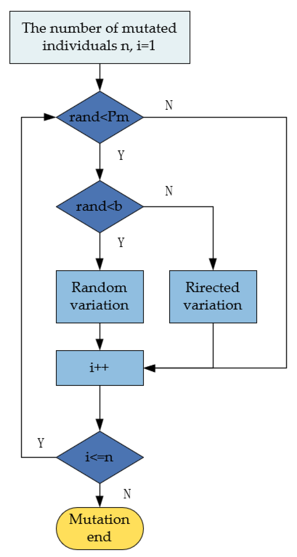
Traditional mutation methods typically rely on single random mutations, but due to the lack of directionality, they often result in difficulties in controlling the quality of the path and may even disrupt individuals with higher fitness, negatively affecting overall optimization performance. Therefore, this paper employs a dual-layer mutation approach. The first layer, random mutation, enhances population diversity, prevents premature convergence, and increases the likelihood of escaping local optima. The second layer, goal-oriented mutation, combines the current search direction to guide the solution towards better regions, thereby improving convergence speed and search efficiency. Furthermore, with the progress of iterations, the dynamic adjustment of layer selection probability enables the algorithm to focus on exploration in the early stages, avoiding premature convergence to local optima while concentrating efforts on searching for better solution regions in the later stages, thus enhancing the convergence speed. The flowchart of the improved mutation strategy is shown in Figure 4.
Figure 4.
Mutation flowchart.
As the iterations progress, the probability of random mutations should gradually reduce to avoid damaging excellent individuals and to accelerate convergence. Therefore, the layer selection probability b needs to be gradually adjusted, and its expression is given by
where B is the layer selection probability, b is the probability adjustment coefficient for selection, t is the current iteration number, and T is the maximum number of iterations.
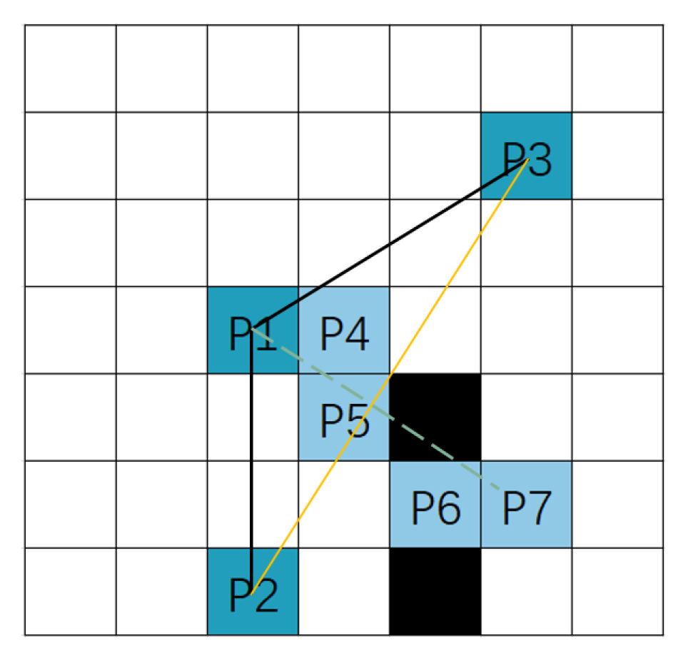
Random mutation is performed by randomly selecting two nodes from the path as mutation nodes and connecting these two nodes using the multi-step method. In reference [26], a target-oriented mutation method is used, where a circular area is drawn with the parent node as the center and a radius 1.4 times the straight-line distance from the parent node to its previous and next nodes. Nodes within the circle are selected as candidate mutation nodes. This results in the traversal of too many mutation nodes, consuming a large amount of hardware resources. To address this, the method in this paper is optimized. First, the two nodes before and after the parent node are connected to form a straight line L1. Then, a perpendicular line L2 is drawn from the parent node to line L1, denoted as L2. Then, the symmetric line L3 of L2 with respect to line L1 is constructed, denoted as L3. Using the improved Bresenham algorithm, we obtain all the grid cells traversed by the straight lines L2 and L3 and designate them as candidate mutation nodes. Then, we use the multi-step method to make the two nodes before and after the parent node pass through the candidate mutation nodes. The probability of selecting each candidate mutation node is given by
where is the probability of selecting the i-th candidate mutation node and is the fitness value of the path formed by the parent node’s adjacent nodes passing through the i-th candidate mutation node. As shown in Figure 5, the black line represents the parental path, with the deep-blue grid P1 indicating the parent node. The deep-blue grids P2 and P3 correspond to the previous and next points relative to the parent node, respectively. The yellow solid line represents line L1, while the green dashed lines represent lines L2 and L3. The light-blue grids P4–P7 represent the candidate mutation nodes.
Figure 5.
Schematic diagram of the goal-oriented mutation method.
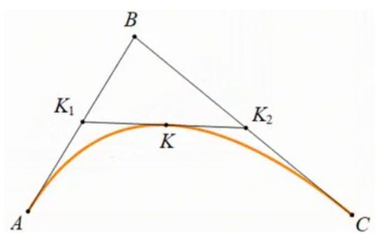
3.5. Bezier Curve Optimization of the Optimal Path
The optimal path generated by the genetic algorithm after iteration consists of multiple line segments, resulting in a non-smooth path. To solve this problem, Bezier curves can be used to optimize the optimal path. A Bezier curve is a curve formed by multiple control points, and the shape of the curve is determined by these control points. As shown in Figure 6, there are three control points, A, B, and C, with , and K satisfying Formula (12). As changes, the point K moves along a trajectory, which is the Bezier curve. The coordinates of K satisfy Formula (13).
Figure 6.
Schematic of Bezier Curve.
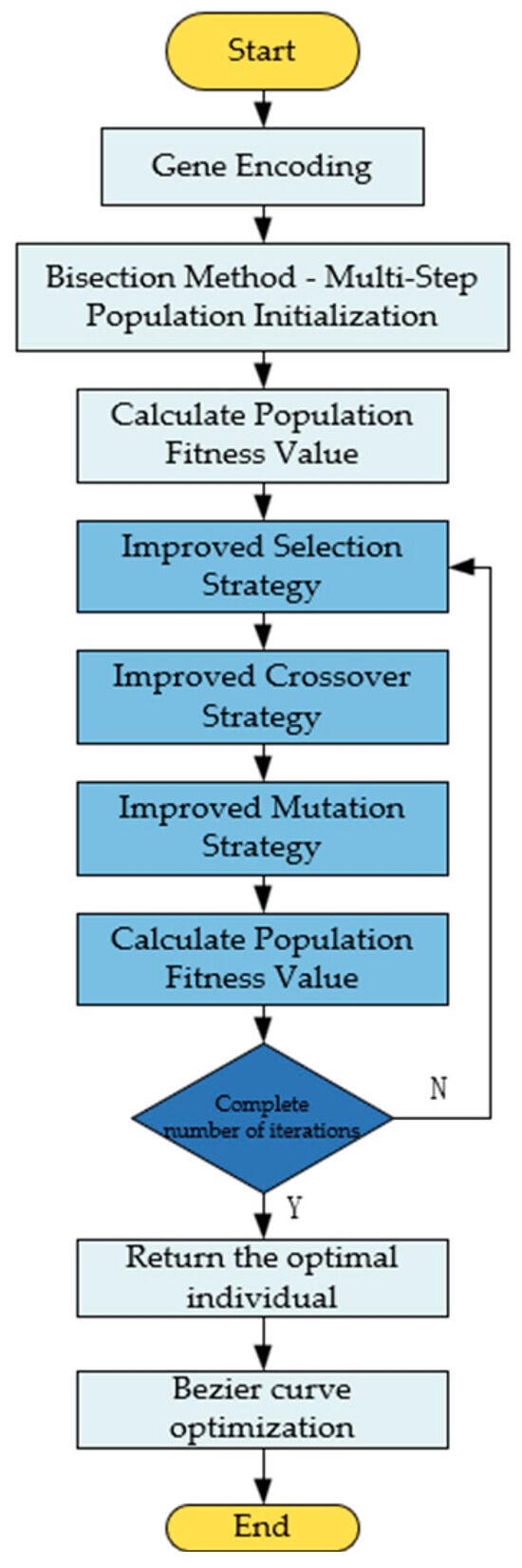
3.6. Algorithm Flow
The algorithm flow of this paper is shown in Figure 7.
Figure 7.
The algorithm flowchart of this paper.
4. Experimental Results and Analysis
In order to verify the effectiveness of the algorithm improvement in this paper, this chapter conducts analysis from both simulation and practical operation perspectives by setting up a MATLAB simulation environment and carrying out mobile-robot real-world navigation experiments.
4.1. MATLAB Simulation Comparison
This paper uses the Windows 11 operating system and MATLAB R2023a simulation platform to set up the experimental environment, where the improved algorithm is verified and compared through simulations. Experiments were conducted on a 20 × 20 grid for the traditional genetic algorithm, the A* algorithm, the method in reference [26] and the algorithm presented in this paper. The goal was to validate the effect of improved population initialization and the overall performance of the improved genetic algorithm. In the experiment, the bottom-left node was set as the starting point, and the top-right node was the endpoint. Table 1 shows the parameter settings, where the values of , K, and b are determined through extensive experiments using the method of controlling variables.
Table 1.
The parameter settings.
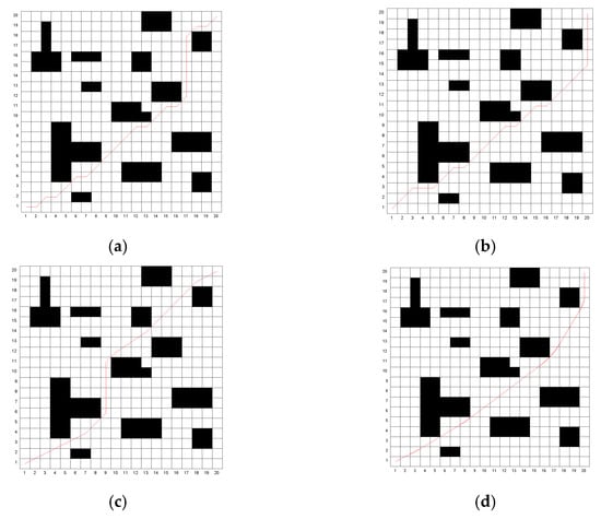
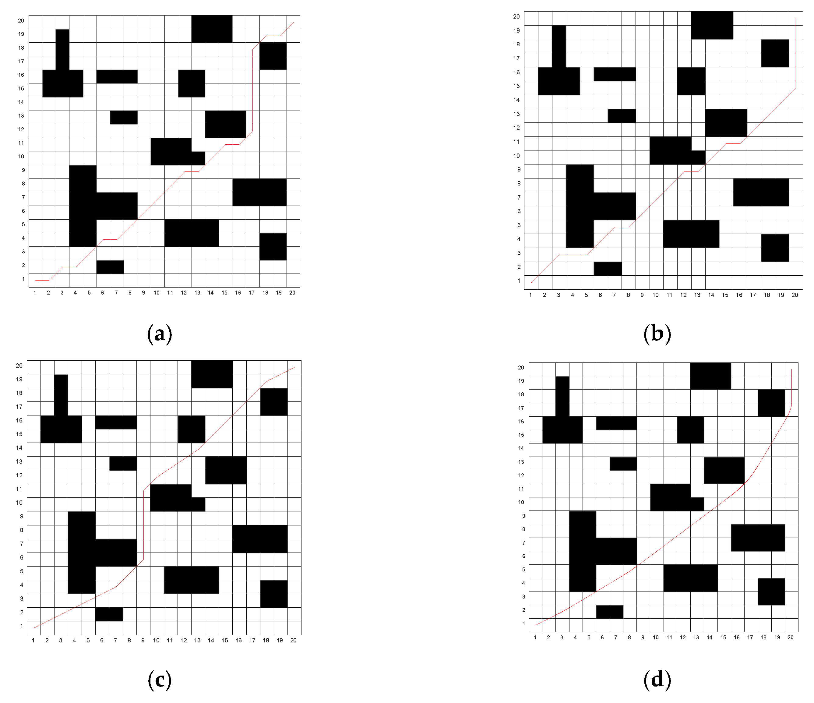
To verify the comprehensive performance of the algorithm, the traditional genetic algorithm, the A* algorithm, the algorithm from reference [26] and the proposed algorithm in this paper are tested for 50 iterations on Map1 and Map2. The experimental results are compared, as shown in Figure 8, Figure 9 and Figure 10 and Table 2.
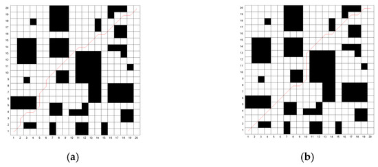
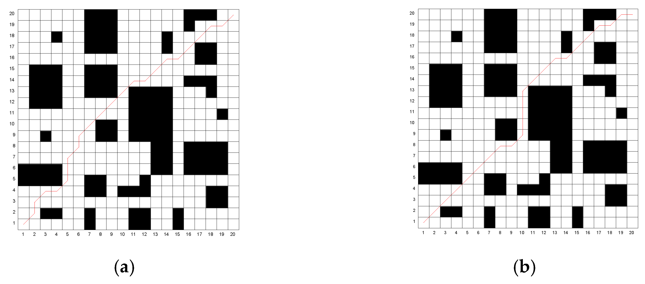
Figure 8.
The optimal paths obtained by the four algorithms on Map 1. (a) Traditional genetic algorithm; (b) A* algorithm; (c) The algorithm in reference [26]; (d) The algorithm in this paper.
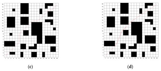
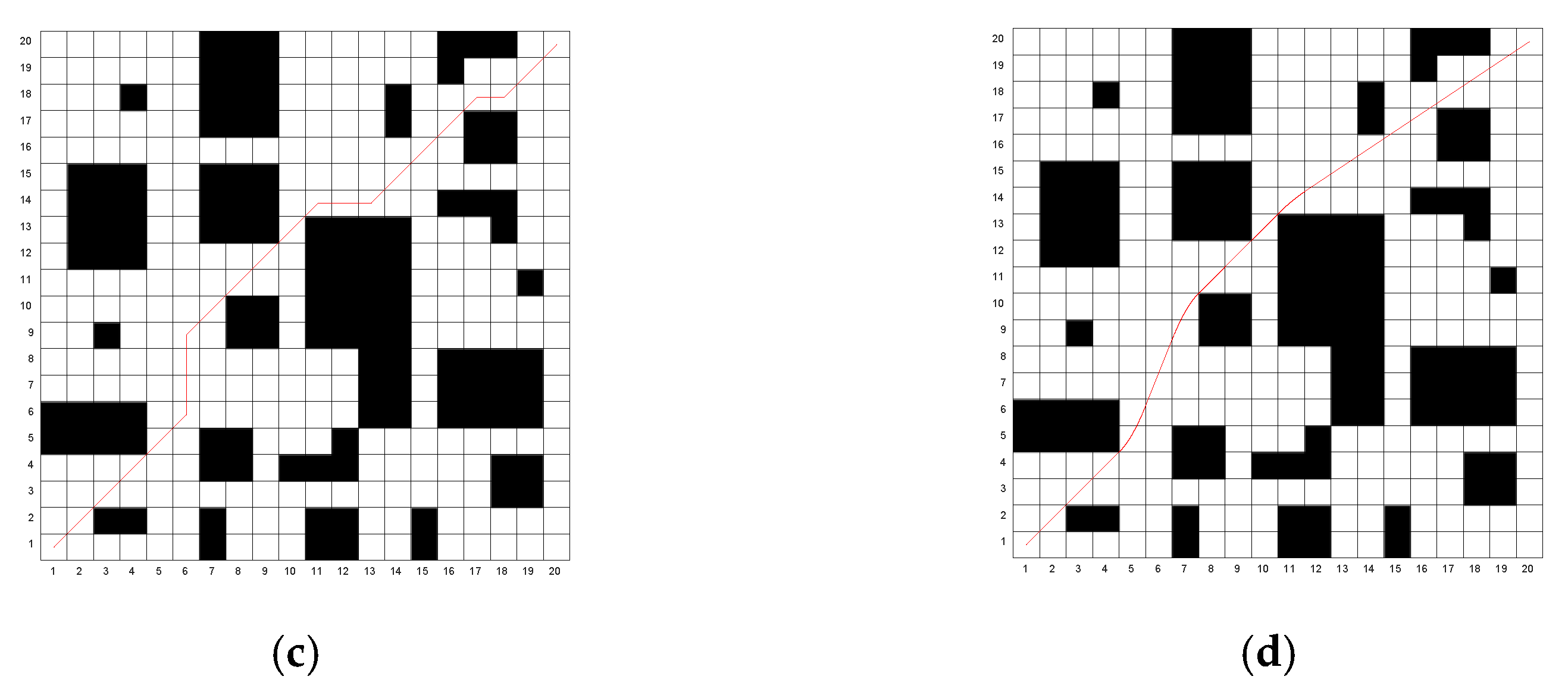
Figure 9.
The optimal paths obtained by the four algorithms on Map 2. (a) Traditional genetic algorithm; (b) A* algorithm; (c) The algorithm in reference [26]; (d) The algorithm in this paper.
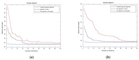
Figure 10.
The iterative process of the optimal path for the three algorithms on Map 1 and Map 2. (a) Map 1; (b) Map 2. Ref. a refers to reference [26].
Table 2.
Comparison of the three algorithms on the data of Map 1 and Map 2.
Through simulation experiments, it can be observed that the traditional algorithm exhibits numerous turning points and lacks smoothness. The algorithm proposed in [26] reduces the number of turning points to some extent. However, the proposed algorithm in this study achieves only three turning points in both Map 1 and Map 2, significantly improving path smoothness. The traditional genetic algorithm converges slowly, while the algorithm in [26] improves the convergence speed. Nevertheless, the proposed algorithm identifies a near-optimal path during the population initialization phase and rapidly converges to the optimal path as iterations proceed, resulting in a shorter average computational time. Although the A* algorithm does not require iteration and has the shortest computation time, the quality of the resulting path is relatively poor. The optimal path lengths obtained using the proposed algorithm are 28.312 m for Map 1 and 27.516 m for Map 2. Compared to the traditional genetic algorithm, A* algorithm and the algorithm in [26], the path length in Map 1 is reduced by 6.5%, 5.2% and 1.9%, respectively, while in Map 2, the reductions are 6.3%, 6.2% and 4%, respectively. The proposed algorithm outperforms all other algorithms in terms of path optimization.
The simulation results show that the dichotomy method and multi-step population initialization significantly improve the path planning performance. Compared with the traditional genetic algorithm, the A* algorithm and the algorithms from references [26], the improved genetic algorithm in this paper demonstrates significant advantages in terms of path length, smoothness, iteration speed, and computational efficiency, with high practical application value.
4.2. Mobile-Robot Navigation Experiment
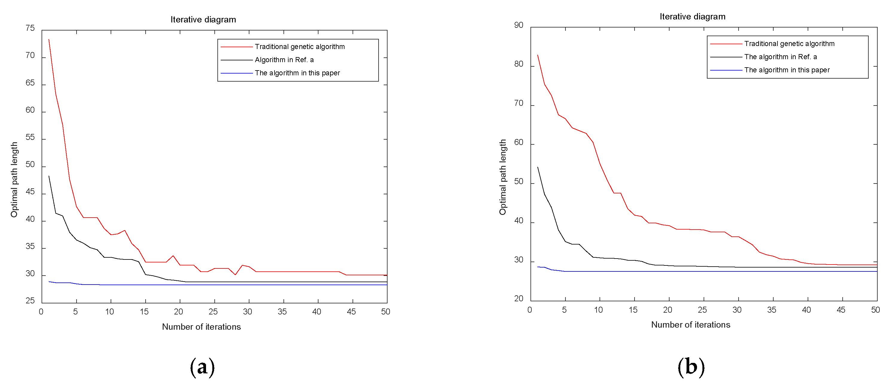
To further validate the performance of the improved algorithm in real-world scenarios, this paper conducts a real-world navigation experiment using the mobile-robot platform shown in Figure 11.
Figure 11.
Mobile-robot platform.
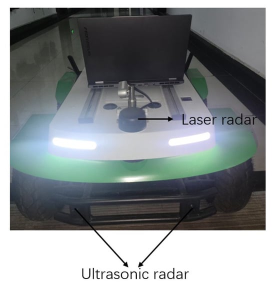
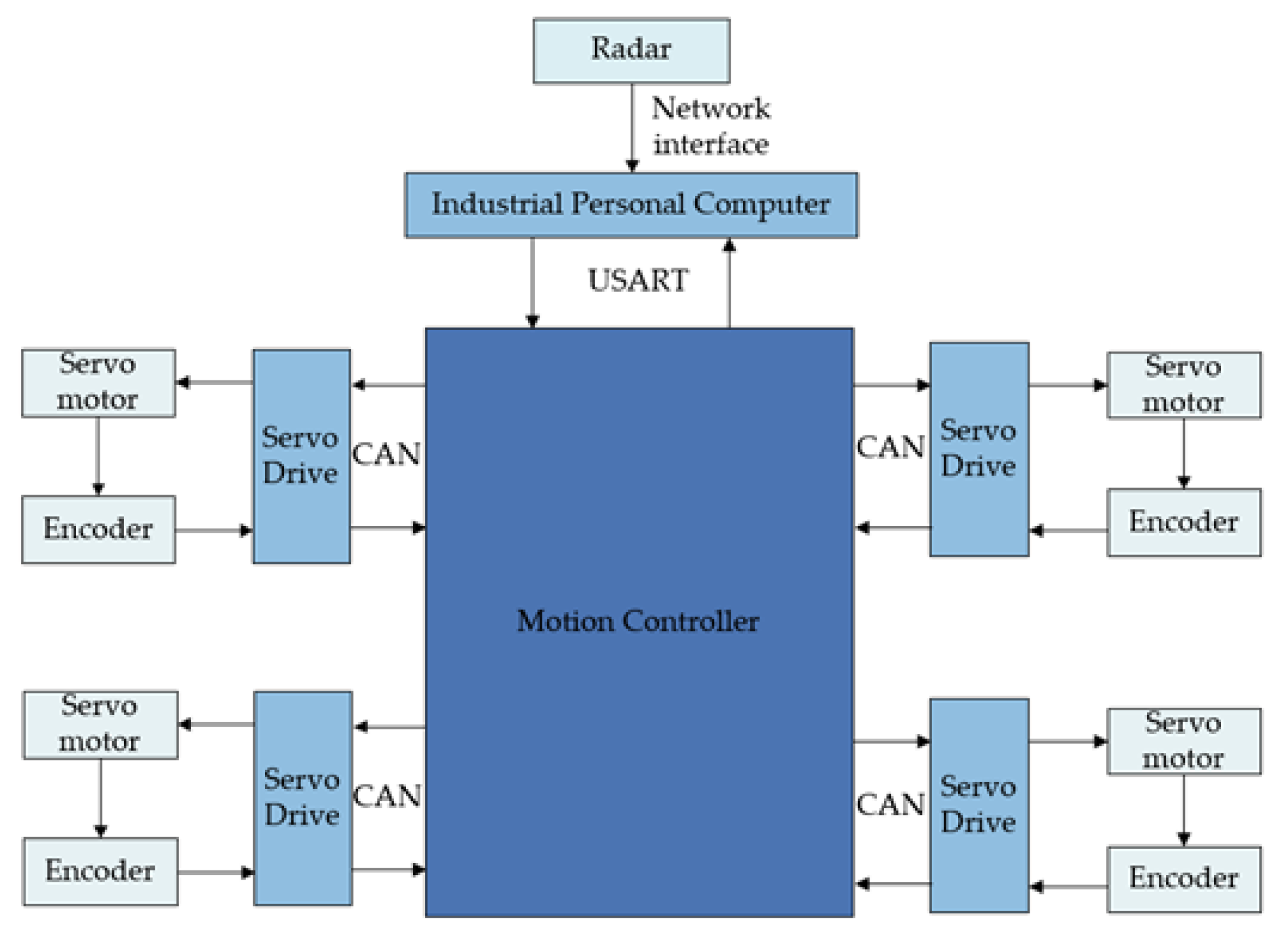
The mobile robot is equipped with an Intel Core i7 series processor, running Ubuntu 18.04 and an ROS1 system. It uses CAN bus communication for driver communication. The robot obtains surrounding information through laser and ultrasonic radar, with a maximum measurement range of 8 unitand a blind spot of 0.2 unit. The radar is connected to the industrial computer via Ethernet for communication. The power system consists of a stable and reliable servo driver, a servo motor, and a 1:40 reducer. The power management system consists of an onboard control board, which manages the power supply to the vehicle. The hardware communication of the mobile robot is shown in Figure 12.
Figure 12.
Schematic diagram of mobile-robot hardware communication.
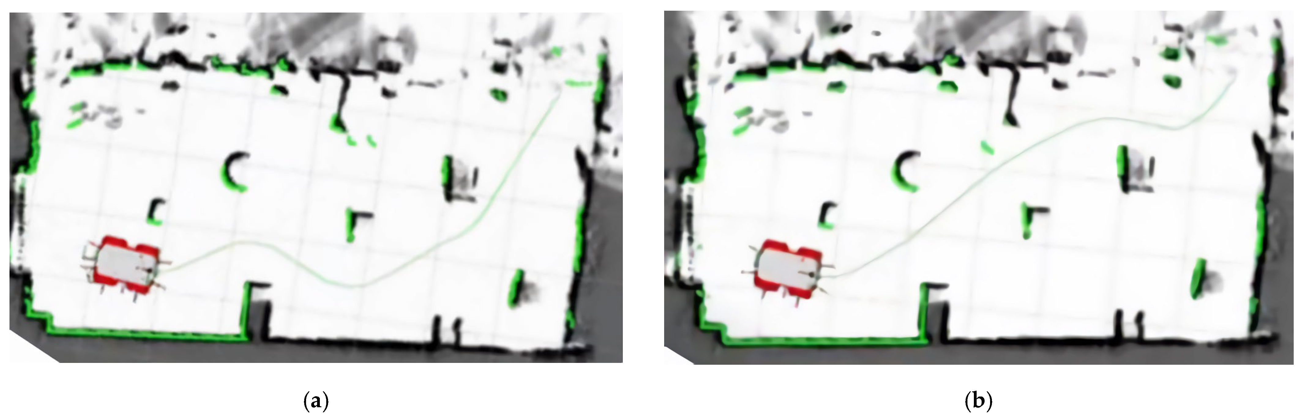
To ensure consistency between the experimental tests and simulation results, we implemented several matching measures: using physical walls to simulate the simulation environment; unifying the test starting and ending points; ensuring the simulation parameters match the actual navigation algorithm; and making the obstacles, terrain, and complexity of the test environment consistent with the simulation. This ensures the reliability and consistency of the experimental results. Under identical experimental conditions (as shown in Figure 13), this paper conducts comparative path planning experiments. The maps are created in an environment built with Gazebo using the Gmapping algorithm and visualized via the Rviz visualization tool. The driving path lengths and smoothness of the mobile robot’s trajectories, planned using the algorithm from reference [26] and the algorithm proposed in this paper, are tested, respectively. The experimental results are compared and illustrated in Figure 14 and Table 3.
Figure 13.
Experimental scenario diagram.
Figure 14.
Paths obtained from navigation using the two algorithms. (a) The algorithm in reference [26]; (b) The algorithm in this paper.
Table 3.
Data comparison of the two algorithms.
Experiments on mobile-robot navigation demonstrate that the improved genetic algorithm proposed in this paper exhibits significant advantages in terms of path length, number of turning points, and the iterations required to achieve the optimal path, further validating the effectiveness of the improved algorithm presented in this paper.
5. Conclusions
This paper addresses the limitations of traditional genetic algorithms in mobile-robot path planning and proposes a path planning method based on an improved genetic algorithm. By using a dichotomy-based multi-step method for population initialization, a tournament selection strategy, an adaptive crossover strategy, a dual-layer encoding mutation strategy, and Bezier curve optimization for the optimal path, the method significantly improves path length, smoothness, iteration speed, and computational efficiency. Experimental results show that the path planning performance of the improved algorithm outperforms traditional genetic algorithms and existing improvement methods, demonstrating high practical value.
However, the improved genetic algorithm proposed in this paper still has certain limitations. Although the improved strategies effectively enhance path quality in static environments, the current experiments mainly focus on static obstacle environments, and the adaptability to moving obstacles has not been fully validated. While the algorithm has been preliminarily validated for feasibility in navigation experiments on a mobile-robot hardware platform (Figure 11 and Table 3), it has not yet been applied in extreme resource-constrained environments, such as low-power microcontrollers. Future research should focus on lightweight algorithm design to reduce high hardware demands and integrate the dynamic window method into the genetic algorithm to achieve dynamic obstacle avoidance.
Author Contributions
Methodology, Z.Z. and H.Y.; Software, S.Z.; Validation, C.X.; Formal analysis, X.B. All authors have read and agreed to the published version of the manuscript.
Funding
This research was funded by Youth Science and Technology Innovation Talent Plan of Hubei Province grant number 2023DJC006.
Institutional Review Board Statement
Not applicable.
Informed Consent Statement
Not applicable.
Data Availability Statement
The original contributions presented in this study are included in the article. Further inquiries can be directed to the corresponding author.
Conflicts of Interest
The authors declare no conflict of interest.
References
- Karur, K.; Sharma, N.; Dharmatti, C.; Siegel, J.E. A Survey of Path Planning Algorithms for Mobile Robots. Vehicles 2021, 3, 448–468. [Google Scholar] [CrossRef]
- Lee, J.; Kim, D.W. An Effective Initialization Method for Genetic Algorithm-Based Robot Path Planning Using a Directed Acyclic Graph. Inf. Sci. 2016, 332, 1–18. [Google Scholar] [CrossRef]
- He, X.; Guo, C. Research on Multi-Strategy Fusion of the Chimpanzee Optimization Algorithm and Its Application in Path Planning. Appl. Sci. 2025, 15, 608. [Google Scholar] [CrossRef]
- Shi, Y.; Huang, S.; Li, M. An Improved Global and Local Fusion Path-Planning Algorithm for Mobile Robots. Sensors 2024, 24, 7950. [Google Scholar] [CrossRef]
- Luo, Z.; Xu, H.; Dai, T. An Ant Colony Path Planning Algorithm Based on Genetic Algorithm Optimized for Logistics Robot. In Proceedings of the 2024 IEEE 4th International Conference on Electronic Technology, Communication and Information, ICETCI 2024, Changchun, China, 24–26 May 2024; Institute of Electrical and Electronics Engineers Inc.: New York, NY, USA, 2024; pp. 711–716. [Google Scholar]
- Han, Y.; Li, C.; An, Z. Based on the Integration of the Improved A* Algorithm with the Dynamic Window Approach for Multi-Robot Path Planning. Appl. Sci. 2025, 15, 406. [Google Scholar] [CrossRef]
- Zhou, X.; Yan, J.; Yan, M.; Mao, K.; Yang, R.; Liu, W. Path Planning of Rail-Mounted Logistics Robots Based on the Improved Dijkstra Algorithm. Appl. Sci. 2023, 13, 9955. [Google Scholar] [CrossRef]
- Dakulovi, M.; Petrovi, I. Two-Way D* Algorithm for Path Planning and Replanning. Rob. Auton. Syst. 2011, 59, 329–342. [Google Scholar] [CrossRef]
- Yang, W.; Wu, P.; Zhou, X.; Lv, H.; Liu, X.; Zhang, G.; Hou, Z.; Wang, W. Improved Artificial Potential Field and Dynamic Window Method for Amphibious Robot Fish Path Planning. Appl. Sci. 2021, 11, 2114. [Google Scholar] [CrossRef]
- Chen, S.; Yang, G.; Cui, G.; Yi, S.; Wu, L. Improved Path Planning and Controller Design Based on PRM. IEEE Access 2025, 13, 44156–44168. [Google Scholar] [CrossRef]
- Zhang, L.; Shi, X.; Yi, Y.; Tang, L.; Peng, J.; Zou, J. Mobile Robot Path Planning Algorithm Based on RRT_Connect. Electronics 2023, 12, 2456. [Google Scholar] [CrossRef]
- Teng, Y.; Feng, T.; Li, J.; Chen, S.; Tang, X. A Dual-Layer Symmetric Multi-Robot Path Planning System Based on an Improved Neural Network-DWA Algorithm. Symmetry 2025, 17, 85. [Google Scholar] [CrossRef]
- Yuan, Q.; Sun, R.; Du, X. Path Planning of Mobile Robots Based on an Improved Particle Swarm Optimization Algorithm. Processes 2023, 11, 26. [Google Scholar] [CrossRef]
- Sun, H.; Zhu, K.; Zhang, W.; Ke, Z.; Hu, H.; Wu, K.; Zhang, T. Emergency Path Planning Based on Improved Ant Colony Algorithm. J. Build. Eng. 2025, 100, 111725. [Google Scholar] [CrossRef]
- Liu, B.; Jin, S.; Li, Y.; Wang, Z.; Zhao, D.; Ge, W. An Asynchronous Genetic Algorithm for Multi-Agent Path Planning Inspired by Biomimicry. J. Bionic Eng. 2025, 22, 851–865. [Google Scholar] [CrossRef]
- Xu, S.; Bi, W.; Zhang, A.; Wang, Y. A Deep Reinforcement Learning Approach Incorporating Genetic Algorithm for Missile Path Planning. Int. J. Mach. Learn. Cybern. 2024, 15, 1795–1814. [Google Scholar] [CrossRef]
- Xu, H.; Niu, Z.; Jiang, B.; Zhang, Y.; Chen, S.; Li, Z.; Gao, M.; Zhu, M. ERRT-GA: Expert Genetic Algorithm with Rapidly Exploring Random Tree Initialization for Multi-UAV Path Planning. Drones 2024, 8, 367. [Google Scholar] [CrossRef]
- Feng, T.; Li, J.; Jiang, H.; Yang, S.X.; Wang, P.; Teng, Y.; Chen, S.; Fu, Q.; Luo, B. The Optimal Global Path Planning of Mobile Robot Based on Improved Hybrid Adaptive Genetic Algorithm in Different Tasks and Complex Road Environments. IEEE Access 2024, 12, 18400–18415. [Google Scholar] [CrossRef]
- Niu, Q.; Fu, Y.; Dong, X. Omnidirectional AGV Path Planning Based on Improved Genetic Algorithm. World Electr. Veh. J. 2024, 15, 166. [Google Scholar] [CrossRef]
- Ning, Y.; Zhang, F.; Jin, B.; Wang, M. Three-Dimensional Path Planning for a Novel Sediment Sampler in Ocean Environment Based on an Improved Mutation Operator Genetic Algorithm. Ocean Eng. 2023, 289, 116142. [Google Scholar] [CrossRef]
- Ab Wahab, M.N.; Nazir, A.; Khalil, A.; Ho, W.J.; Akbar, M.F.; Noor, M.H.M.; Mohamed, A.S.A. Improved Genetic Algorithm for Mobile Robot Path Planning in Static Environments. Expert Syst. Appl. 2024, 249, 123762. [Google Scholar] [CrossRef]
- Lamini, C.; Benhlima, S.; Elbekri, A. Genetic Algorithm Based Approach for Autonomous Mobile Robot Path Planning. Procedia Comput. Sci. 2018, 127, 180–189. [Google Scholar] [CrossRef]
- Cai, Y.; Liu, H.; Li, M.; Ren, F. A Method of Dual-AGV-Ganged Path Planning Based on the Genetic Algo-rithm. Appl. Sci. 2024, 14, 7482. [Google Scholar] [CrossRef]
- Han, J.; Li, W.; Xia, W.; Wang, F. Research on Complete Coverage Path Planning of Agricultural Robots Based on Markov Chain Improved Genetic Algorithm. Appl. Sci. 2024, 14, 9868. [Google Scholar] [CrossRef]
- Sarkar, R.; Barman, D.; Chowdhury, N. Domain Knowledge Based Genetic Algorithms for Mobile Robot Path Planning Having Single and Multiple Targets. J. King Saud. Univ.-Comput. Inf. Sci. 2022, 34, 4269–4283. [Google Scholar] [CrossRef]
- Wang, L.; Wang, Y.; Li, D.; Wang, T. Research on Path Planning of Mobile Robot Based on Improved Genetic Algorithm. Huazhong Keji Daxue Xuebao (Ziran Kexue Ban)/J. Huazhong Univ. Sci. Technol. (Nat. Sci. Ed.) 2024, 52, 158–164. [Google Scholar] [CrossRef]


Disclaimer/Publisher’s Note: The statements, opinions and data contained in all publications are solely those of the individual author(s) and contributor(s) and not of MDPI and/or the editor(s). MDPI and/or the editor(s) disclaim responsibility for any injury to people or property resulting from any ideas, methods, instructions or products referred to in the content. |
© 2025 by the authors. Licensee MDPI, Basel, Switzerland. This article is an open access article distributed under the terms and conditions of the Creative Commons Attribution (CC BY) license (https://creativecommons.org/licenses/by/4.0/).