
Wind Field Simulation and Its Impacts on Athletes’ Performance, Based on the Computational Fluid Dynamics Method: A Case Study of the National Sliding Centre of the Beijing 2022 Winter Olympics


Abstract
1. Introduction
2. Materials and Methods
2.1. Study Area and Meteorological Dataset
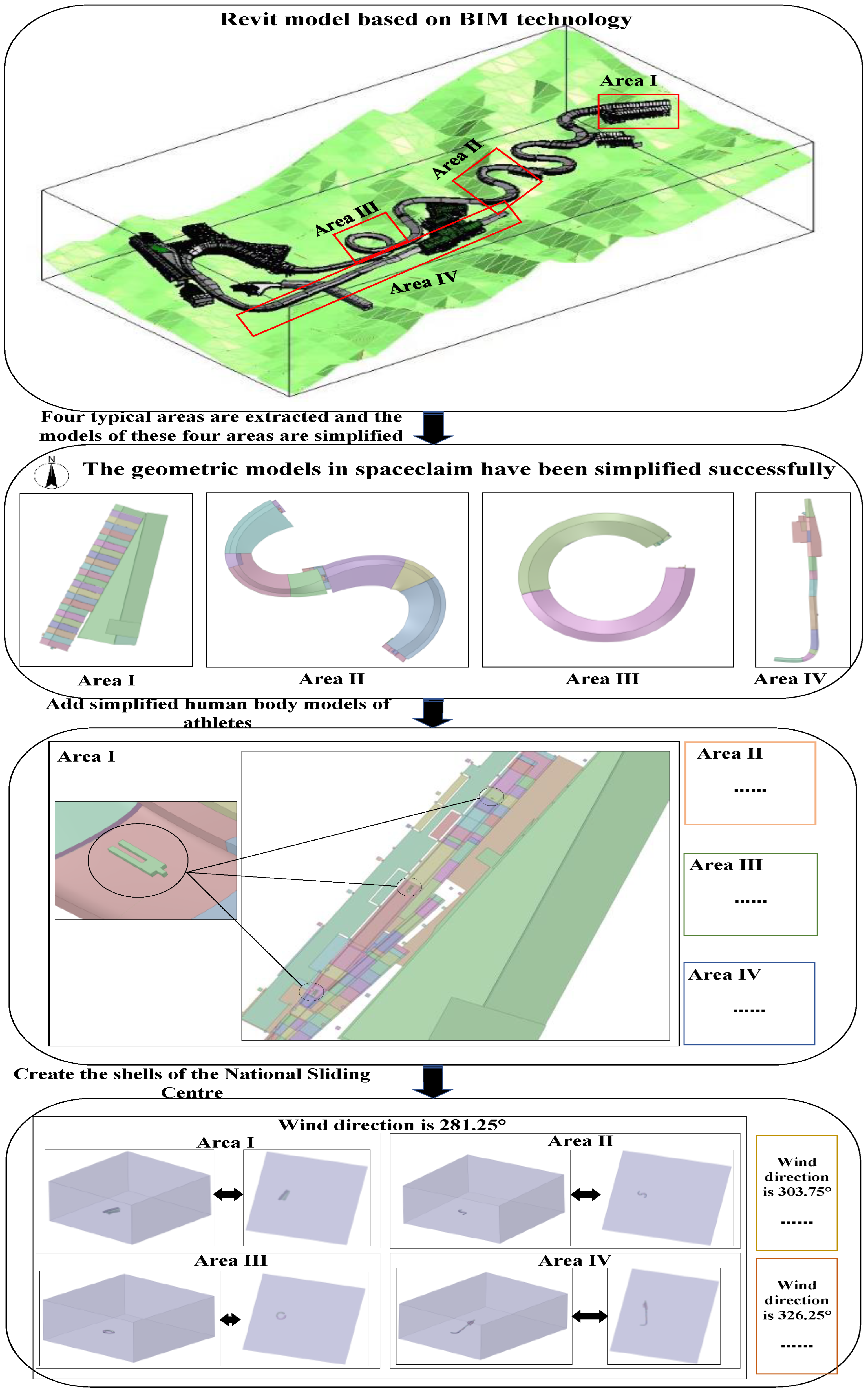
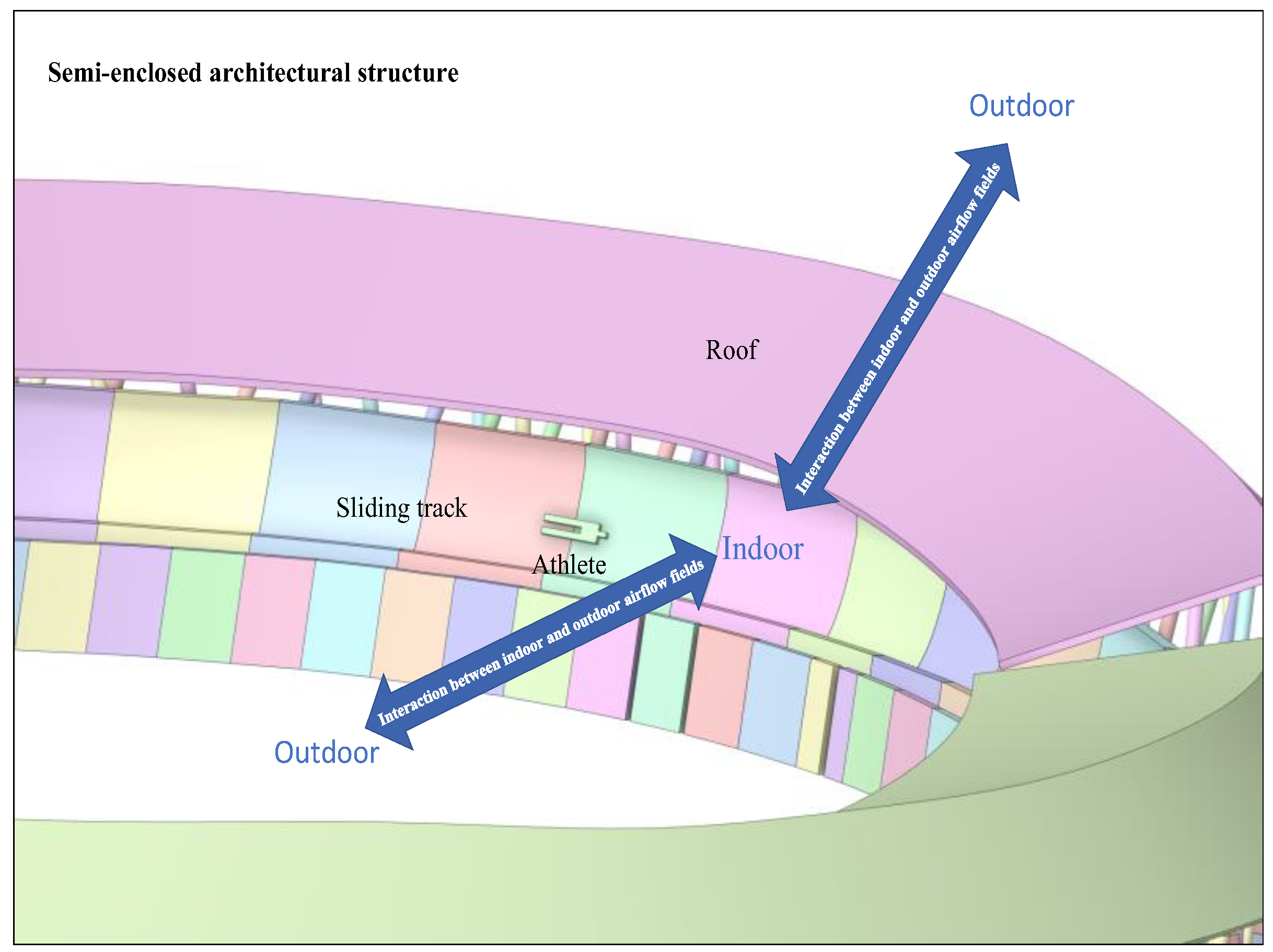
2.2. Establishment of Geometric Model
2.3. CFD Simulation Method and Parameter Setting
2.3.1. CFD Simulation Principle
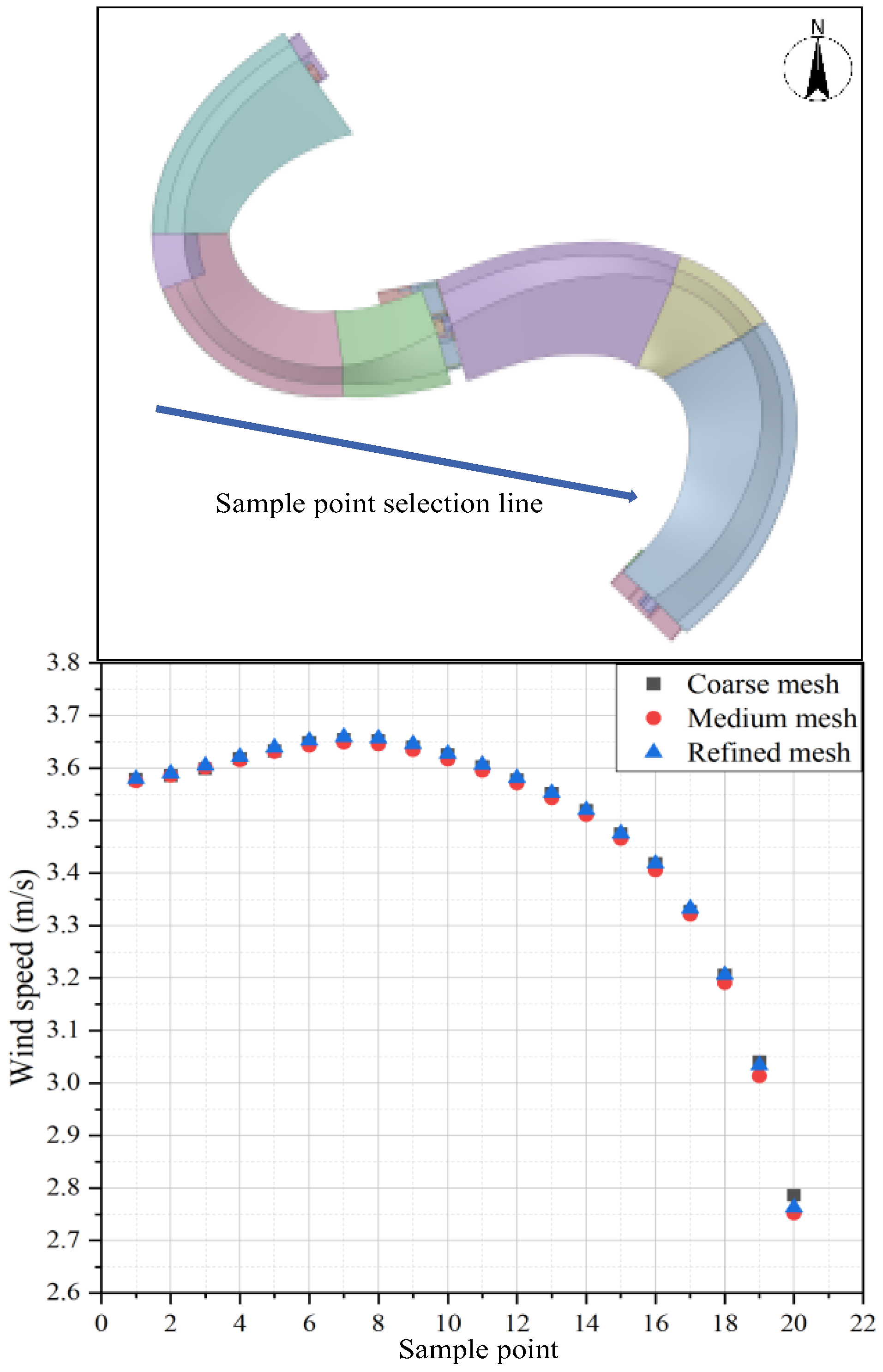
2.3.2. Meshing and Independence Verification
2.3.3. CFD Boundary and Input Parameter Setting
3. Construction of Parameter Indicators for Analysis of Wind Field Characteristics
3.1. Wind Speed Dispersion Index
3.1.1. Global Wind Speed Dispersion
3.1.2. Local Wind Speed Dispersion
3.2. Construction and Quantification of Main Influencing Parameters on Athletes’ Competition Performance
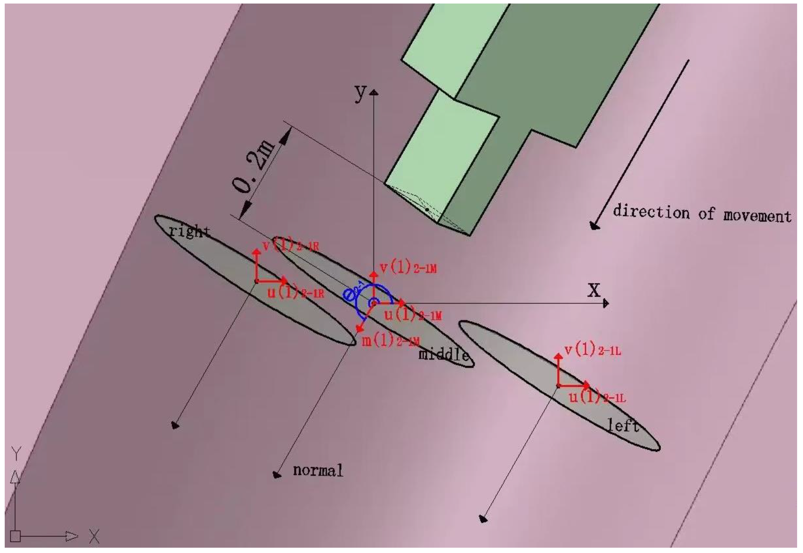
3.2.1. Athletes’ Normal Average Headwind Resistance
3.2.2. Average Wind Resistance over Entire Journey
3.2.3. Wind Resistance Reduction Indicators of Optimized Sliding Route
4. Characteristics of Outdoor Wind Field at National Sliding Centre
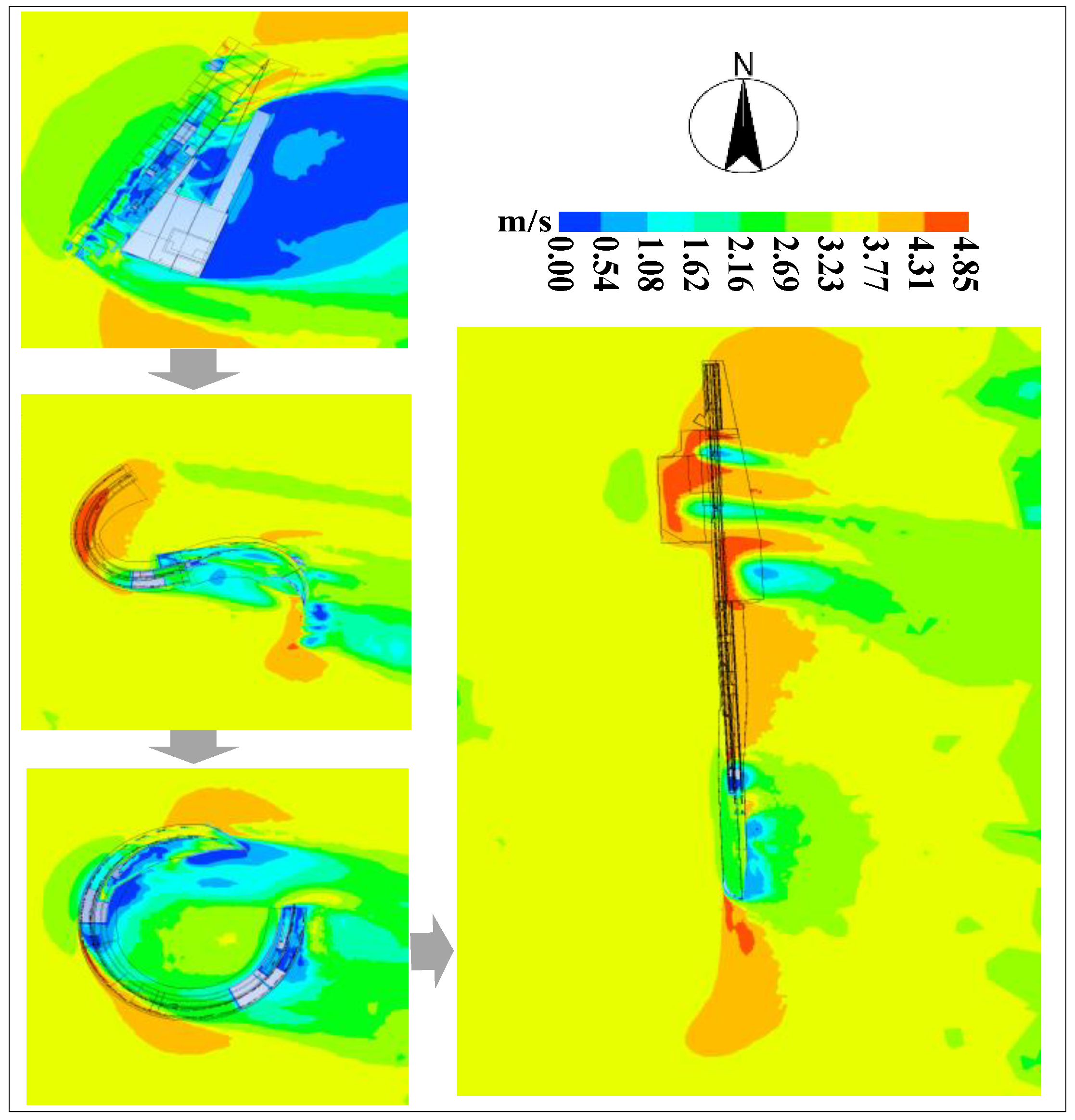
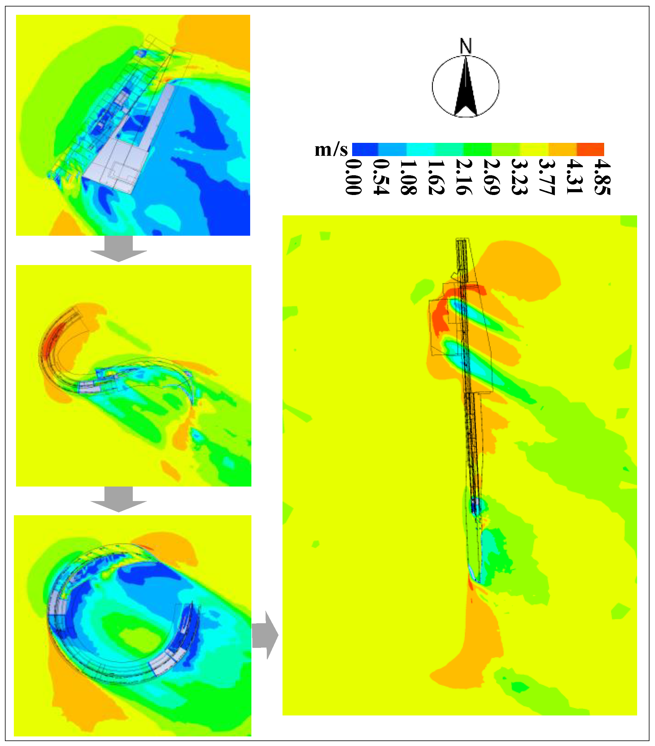
4.1. Analysis of Outdoor Wind Field Distribution Characteristics
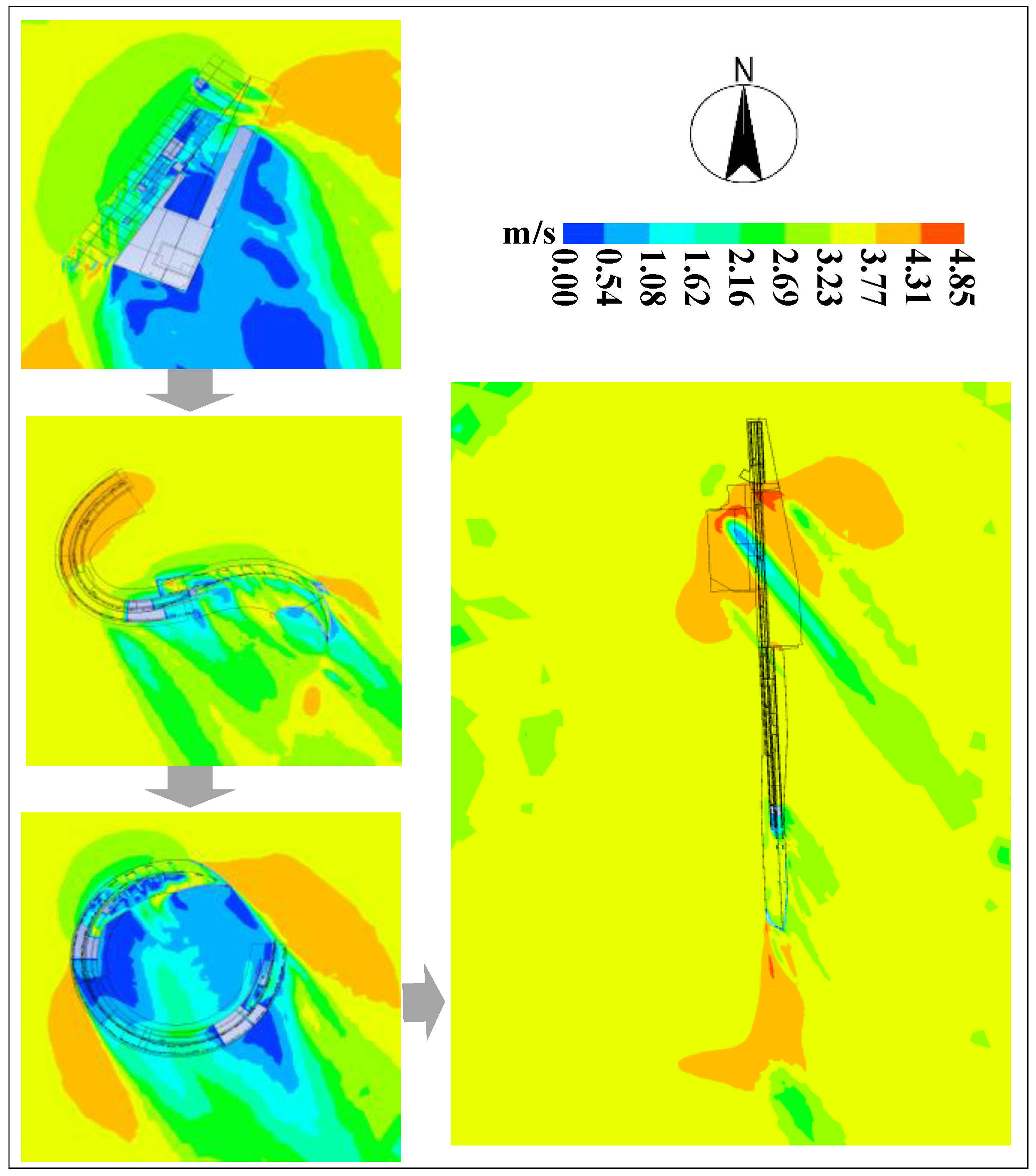
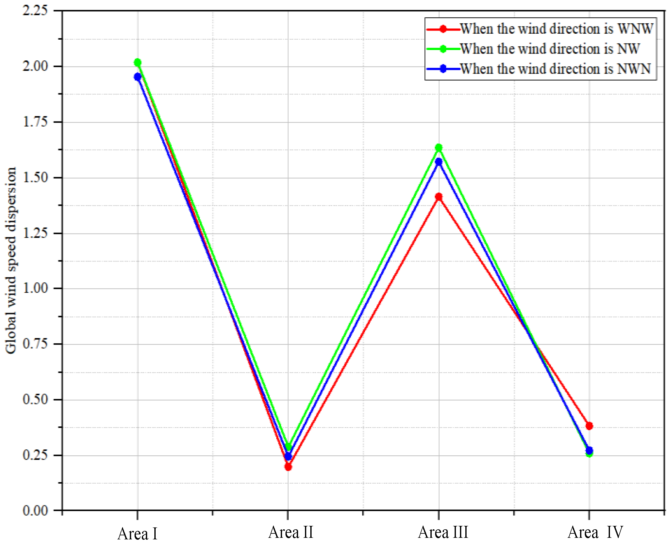
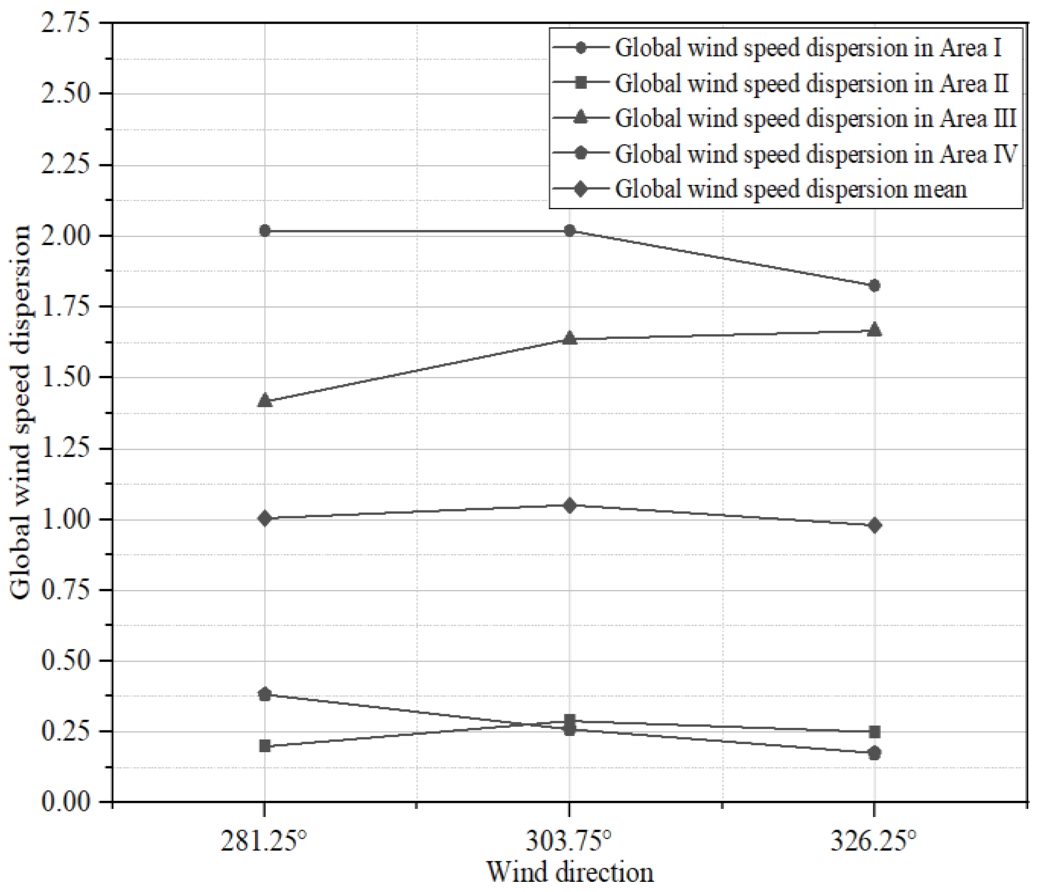
4.2. Comparative Analysis of Outdoor Wind Field Characteristics
5. Analysis and Discussion of Influence of Wind Resistance on Athletes
5.1. Calculation and Analysis of Average Wind Resistance over Entire Journey
5.2. Optimization of Athletes’ Sliding Routes
5.3. Analysis of Wind Resistance Reduction of Optimized Sliding Route
6. Conclusions
Supplementary Materials
Author Contributions
Funding
Institutional Review Board Statement
Informed Consent Statement
Data Availability Statement
Conflicts of Interest
Abbreviations
| NAHR | Normal average headwind resistance |
| RNAHR | Relative value of normal average headwind resistance |
| AWREJ | Average wind resistance over entire journey |
| WRDUI | Wind resistance reduction index of optimized sliding route |
| TS | Time saved of optimized sliding route |
| AWRDU | Average wind resistance reduction of optimized sliding route |
Appendix A

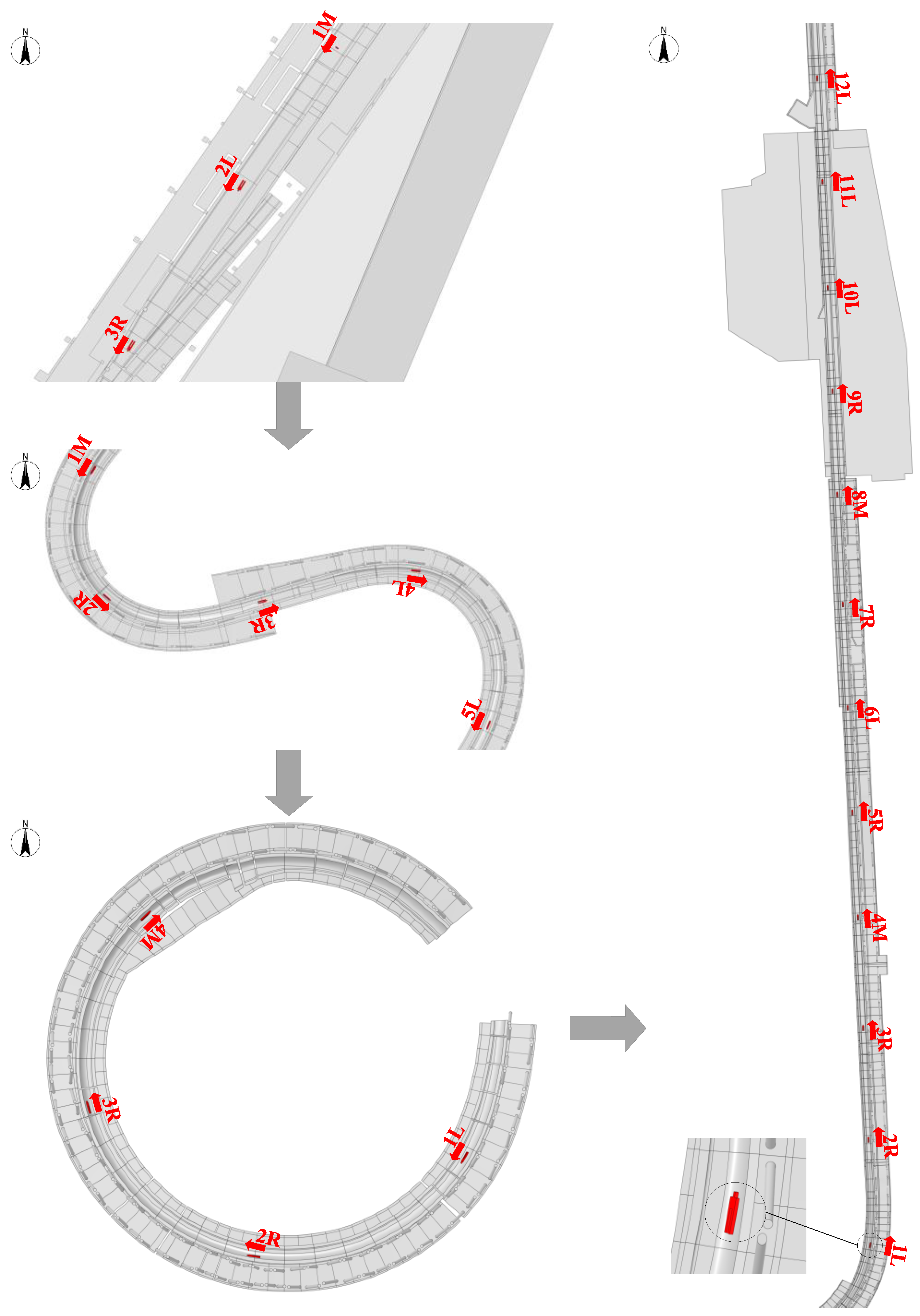
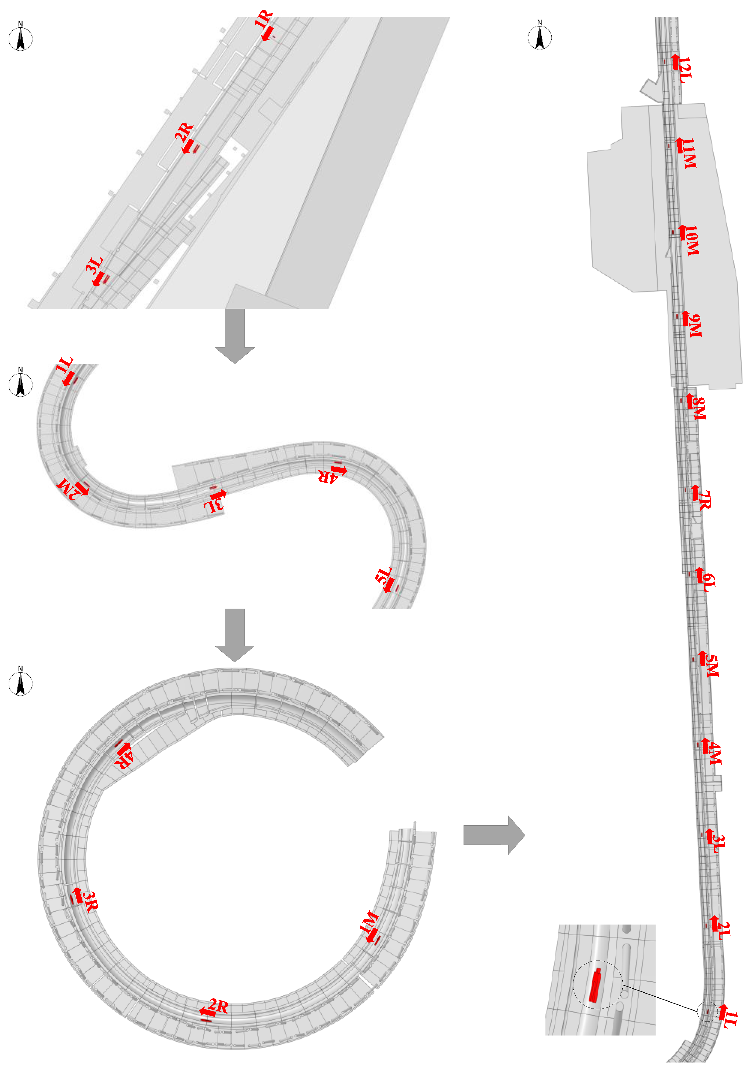
| Wind Direction | Area | Sliding Route Suggestion |
|---|---|---|
| WNW | Area I | 1M−2M-3R |
| Area II | 1R-2R-3M-4R-5R | |
| Area III | 1M-2R-3L-4L | |
| Area IV | 1L-2L-3M-4M-5M-6M-7R-8L-9L-10R -11L-12R | |
| NW | Area I | 1M-2L-3R |
| Area II | 1M-2R-3R-4L-5L | |
| Area III | 1L-2R-3R-4M | |
| Area IV | 1L-2R-3R-4M-5R-6L-7R-8M-9R-10L -11L-12L | |
| NWN | Area I | 1R-2R-3L |
| Area II | 1L-2M-3L-4R-5L | |
| Area III | 1M-2R-3R-4R | |
| Area IV | 1L-2L-3L-4M-5M-6L-7R-8M-9M-10M -11M-12L |
| Wind Level | Wind Direction | Suggestion of Athletes’ Sliding Routes |
|---|---|---|
| 3.5 | WNW | Area I (1M-2R-3R), Area II (1R-2R-3M-4R-5R), Area III (1M-2R-3R-4L), Area IV (1L-2L-3M-4M-5M-6M-7R-8L-9L-10R-11L-12R) |
| NW | Area I (1M-2L-3R), Area II (1R-2R-3R-4L-5L), Area III (1L-2R-3R-4M), Area IV (1L-2R-3R-4M-5R-6L-7R-8M-9R-10L-11L-12L) | |
| NWN | Area I (1R-2R-3L), Area II (1M-2R-3R-4R-5L), Area III (1M-2R-3R-4R), Area IV (1L-2L-3L-4M-5M-6L-7R-8M-9M-10M-11M-12L) | |
| 4.5 | WNW | Area I (1M-2R-3R), Area II (1L-2R-3M-4R-5R), Area III (1L-2R-3R-4L), Area IV (1L-2L-3M-4M-5M-6M-7R-8L-9L-10R-11L-12R) |
| NW | Area I (1M-2L-3R), Area II (1R-2R-3R-4L-5L), Area III (1L-2R-3R-4M), Area IV (1L-2R-3R-4M-5R-6L-7M-8M-9R-10L-11L-12R) | |
| NWN | Area I (1R-2R-3L), Area II (1M-2M-3R-4R-5L), Area III (1M-2R-3R-4R), Area IV (1L-2L-3L-4M-5M-6L-7R-8M-9M-10M-11M-12L) | |
| 5.5 | WNW | Area I (1M-2R-3R), Area II (1M-2R-3M-4R-5R), Area III (1L-2R-3M-4L), Area IV (1L-2L-3M-4M-5M-6M-7R-8L-9L-10R-11L-12R) |
| NW | Area I (1M-2L-3R), Area II (1M-2R-3R-4L-5L), Area III (1L-2R-3L-4M), Area IV (1L-2R-3R-4M-5R-6L-7M-8M-9R-10R-11L-12R) | |
| NWN | Area I (1R-2R-3L), Area II (1R-2M-3R-4L-5L), Area III (1M-2R-3R-4R), Area IV (1L-2L-3L-4M-5M-6L-7R-8M-9M-10M-11M-12L) | |
| 6.5 | WNW | Area I (1M-2M-3R), Area II (1L-2R-3M-4R-5R), Area III (1M-2R-3R), Area IV (1L-2L-3M-4M-5M-6M-7R-8L-9L-10R-11L-12R) |
| NW | Area I (1M-2L-3R), Area II (1L-2R-3R-4L-5L), Area III (1L-2R-3R-4L), Area IV (1L-2R-3R-4M-5R-6L-7M-8M-9R-10L-11L-12R) | |
| NWN | Area I (1R-2R-3L), Area II (1R-2M-3L-4R-5L), Area III (1M-2R-3R-4R), Area IV (1L-2L-3L-4M-5M-6L-7R-8M-9M-10M-11M-12L) | |
| 7.5 | WNW | Area I (1M-2R-3R), Area II (1R-2R-3M-4R-5R), Area III (1M-2R-3R-4L), Area IV (1L-2L-3M-4M-5M-6M-7R-8L-9L-10R-11L-12R) |
| NW | Area I (1M-2L-3R), Area II (1L-2R-3R-4L-5L), Area III (1L-2R-3R-4L), Area IV (1L-2R-3R-4M-5R-6L-7M-8M-9R-10R-11L-12M) | |
| NWN | Area I (1R-2R-3L), Area II (1L-2M-3R-4R-5L), Area III (1M-2R-3R-4R), Area IV (1L-2L-3L-4M-5M-6L-7R-8M-9M-10M-11M-12L) | |
| 8.229 | WNW | Area I (1M-2M-3R), Area II (1R-2R-3M-4R-5R), Area III (1L-2R-3L-4L), Area IV (1L-2L-3M-4M-5M-6M-7R-8L-9L-10R-11R-12R) |
| NW | Area I (1M-2L-3R), Area II (1L-2R-3R-4L-5L), Area III (1L-2R-3R-4M), Area IV(1L-2R-3R-4M-5R-6L-7M-8M-9R-10R-11L-12R) | |
| NWN | Area I (1R-2R-3L), Area II (1M-2M-3R-4R-5L), Area III (1M-2M-3R-4R-5L), Area IV(1L-2L-3L-4M-5M-6L-7R-8M-9M-10M-11M-12L) |
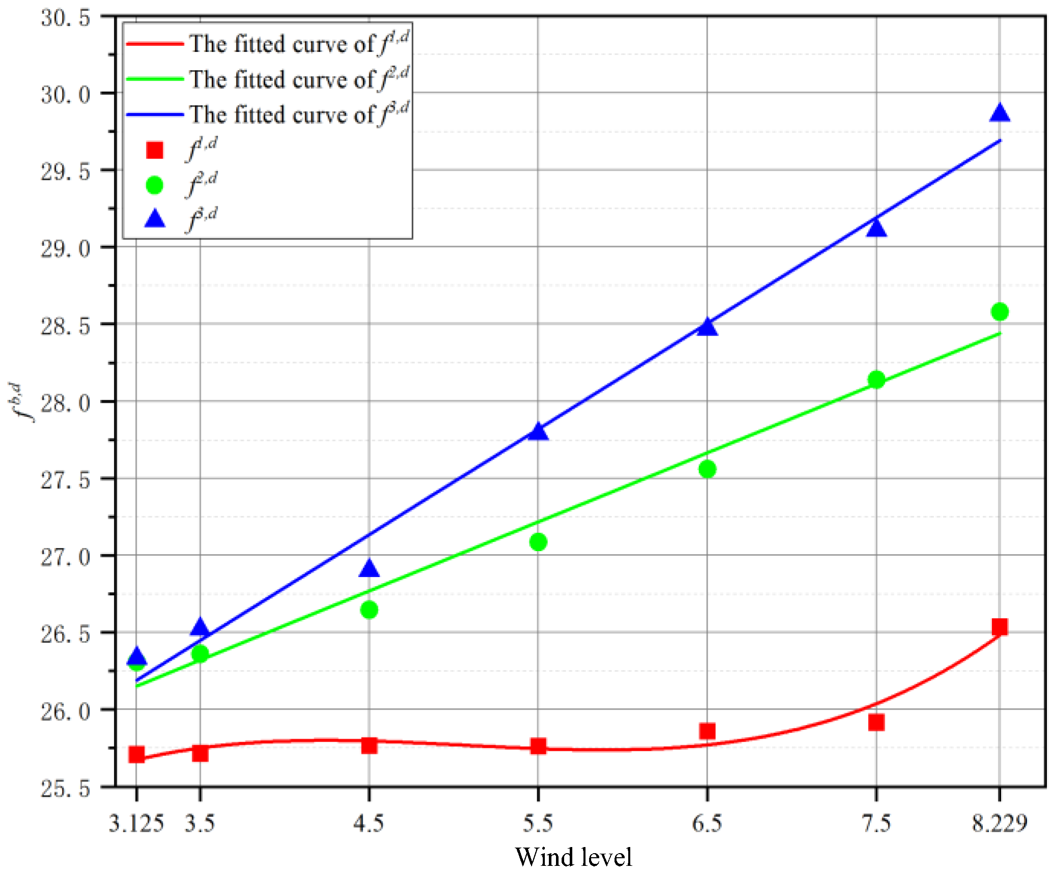
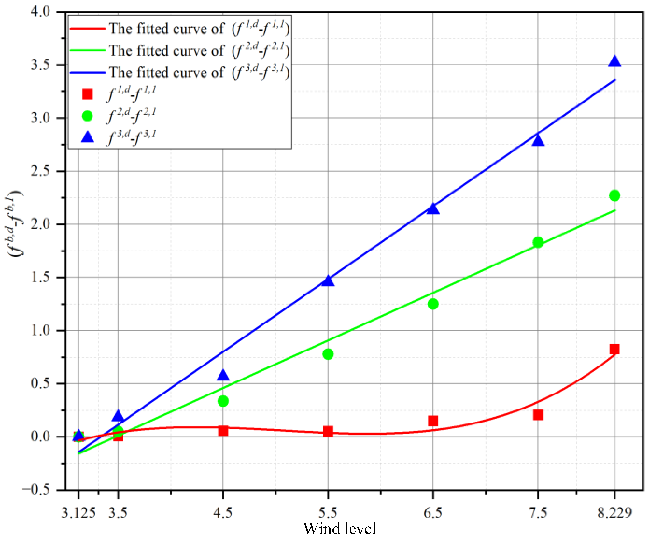
| Wind Direction | WNW | NW | NWN |
|---|---|---|---|
| (N) | 25.7153 | 26.3604 | 26.5214 |
| - (N) | 0.0070 | 0.0517 | 0.1880 |
| (N) | 25.7662 | 26.6459 | 26.6459 |
| - (N) | 0.0579 | 0.3371 | 0.5687 |
| (N) | 25.7609 | 27.0870 | 27.7898 |
| - (N) | 0.0525 | 0.7782 | 1.4563 |
| (N) | 25.8585 | 27.5592 | 28.4683 |
| - (N) | 0.1502 | 1.2504 | 2.1349 |
| (N) | 25.9155 | 28.1387 | 29.1085 |
| - (N) | 0.2072 | 1.8300 | 2.7751 |
| (N) | 26.5345 | 28.5795 | 29.8574 |
| - (N) | 0.8262 | 2.2707 | 3.5240 |
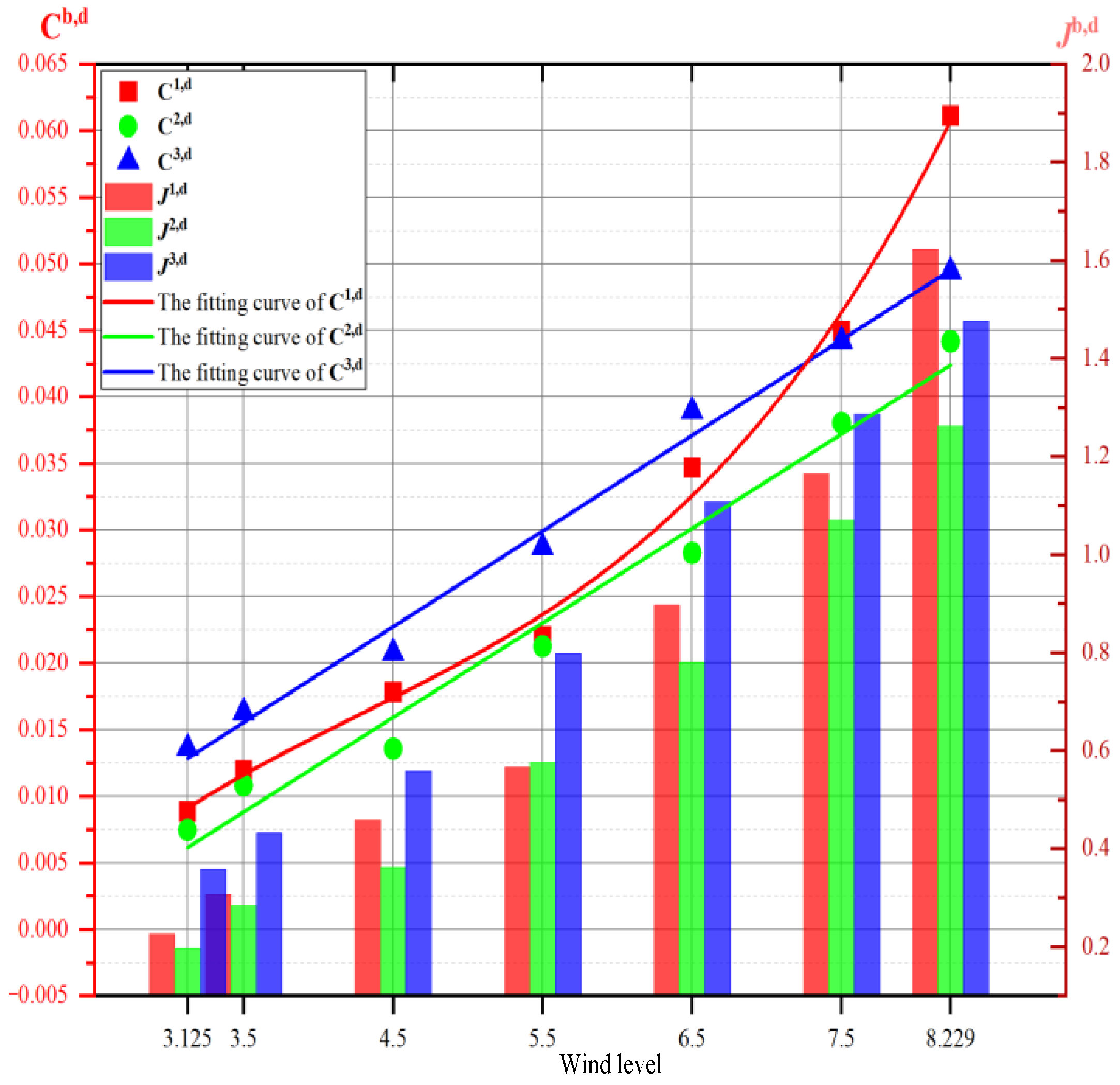
| Jb,d(N) | Wind Direction | ||||
|---|---|---|---|---|---|
| WNW | NW | NWN | Mean Value | ||
| Wind level | 3.125 | 0.2274 | 0.1962 | 0.3586 | 0.2607 |
| 3.5 | 0.3074 | 0.2847 | 0.4325 | 0.3415 | |
| 4.5 | 0.4593 | 0.362 | 0.5588 | 0.4600 | |
| 5.5 | 0.5668 | 0.5759 | 0.798 | 0.6469 | |
| 6.5 | 0.8971 | 0.7795 | 1.1083 | 0.9283 | |
| 7.5 | 1.165 | 1.0706 | 1.2866 | 1.1741 | |
| 8.229 | 1.6224 | 1.2624 | 1.4756 | 1.4535 | |
References
- Zhang, X.; Weerasuriya, A.; Tse, K.T. CFD Simulation of Natural Ventilation of a Generic Building in Various Incident Wind Directions: Comparison of Turbulence Modelling, Evaluation Methods, and Ventilation Mechanisms. Energy Build. 2020, 229, 110516. [Google Scholar]
- Tavakol, M.M.; Yaghoubi, M.; Ahmadi, G. Experimental and numerical analysis of airflow around a building model with an array of domes. J. Build. Eng. 2020, 34, 101901. [Google Scholar]
- Kareem, A. Emerging frontiers in wind engineering: Computing, stochastics, machine learning and beyond. J. Wind Eng. Ind. Aerodyn. 2020, 206, 104320. [Google Scholar]
- Chen, G.; Rong, L.; Zhang, G. Unsteady-state CFD simulations on the impacts of urban geometry on outdoor thermal comfort within idealized building arrays. Sustain. Cities Soc. 2021, 74, 103187. [Google Scholar]
- Hu, X.; Zhang, S.; Xie, Z. Effects of corner recession on the aerodynamic characteristics of tall buildings with various side ratios: Experimental and numerical study. J. Build. Eng. 2024, 109832. [Google Scholar]
- Xu, Y.; Wang, W.; Chen, B.; Chang, M.; Wang, X. Identification of ventilation corridors using backward trajectory simulations in Beijing. Sustain. Cities Soc. 2021, 70, 102889. [Google Scholar]
- Heusinkveld, B.G.; Steeneveld, G.V.; Van Hove, L.W.A.; Jacobs, C.M.J.; Holtslag, A.A.M. Spatial variability of the Rotterdam urban heat island as influenced by urban land use. J. Geophys. Res. Atmos. 2014, 119, 677–692. [Google Scholar]
- Zhang, H.; Gao, Z.; Ding, W.; Zhang, W. Numerical study of the impact of green space layout on microclimate. Procedia Eng. 2017, 205, 1762–1768. [Google Scholar]
- Sabrin, S.; Karimi, S.; Nazari, R. The cooling potential of various vegetation covers in a heat-stressed underserved community in the deep south: Birmingham. Alabama. Urban Clim. 2023, 51, 101623. [Google Scholar]
- Guo, W.; Liu, W.; Yuan, X. Study on natural ventilation design optimization based on CFD simulation for green buildings. Procedia Eng. 2015, 121, 573–581. [Google Scholar] [CrossRef]
- Węgrzyński, W.; Krajewski, G.; Kimbar, G.; Lipecki, T. Fire smoke dispersion inside and outside of a warehouse building in moderate and strong wind conditions. Fire Saf. J. 2023, 136, 103760. [Google Scholar]
- Zhou, R.; Seong, R.; Liu, J. Review of the development of hydrological data quality control in Typhoon Committee Members. Trop. Cyclone Res. Rev. 2024, 13, 113–124. [Google Scholar]
- Skamarock, W.C.; Klemp, J.B.; Dudhia, J.; Gill, D.O.; Liu, Z.; Berner, J.; Wang, W.; Powers, J.G.; Duda, M.G.; Barker, D.M. A Description of the Advanced Research WRF, version 4; NCAR tech. note ncar/tn-556+ str; National Center for Atmospheric Research: Boulder, CO, USA, 2019; p. 145. [Google Scholar]
- Kopp, G.A.; Khezeli, M.; Srebric, J. A review of CFD simulations of wind effects on outdoor thermal comfort. Build. Environ. 2015, 91, 3–15. [Google Scholar]
- Wilke, U. Computational fluid dynamics for urban physics: Importance, scales, possibilities, limitations and ten tips and tricks towards accurate and reliable simulations. Build. Simul. 2018, 11, 703–723. [Google Scholar]
- Lim, J.; Ooka, R. A CFD-Based optimization of building configuration for urban ventilation potential. Energies 2021, 14, 1447. [Google Scholar] [CrossRef]
- Iqbal, Q.M.Z.; Chan, A.L.S. Pedestrian level wind environment assessment around group of high-rise cross-shaped buildings: Effect of building shape, separation and orientation. Build. Environ. 2016, 101, 45–63. [Google Scholar] [CrossRef]
- Verma, S.K.; Roy, A.K.; Lather, S.; Sood, M. CFD simulation for wind load on octagonal tall buildings. Int. J. Eng. Trends Technol. 2015, 24, 211–216. [Google Scholar] [CrossRef]
- Dong, X.; Qi, Y.; Wang, W.; Fu, P.; Peng, T.; Qi, Q.Y. Simulation study on emergency evacuation of fire personnel in high-rise building: A case study of hospital. China Emerg. Rescue Rescue 2024, 30–37. (In Chinese) [Google Scholar]
- Tan, Z.C.; Fang, Z.; Jiang, Y.X. Analysis of air flow organization in a sports stadium. Green Build. 2020, 12, 57–59. (In Chinese) [Google Scholar]
- Koopmann, T.; Faber, I.; Baker, J.; Schorer, J. Assessing technical skills in talented youth athletes: A systematic review. Sports Med. 2020, 50, 1593–1611. [Google Scholar]
- Wilson, N.; Thomson, A.; Riches, P. Development and presentation of the first design process model for sports equipment design. Res. Eng. Des. 2017, 28, 495–509. [Google Scholar]
- Santi, G.; Williams, G.; Mellalieu, S.D.; Wadey, R.; Carraro, A. The athlete psychological well-being inventory: Factor equivalence with the sport injury-related growth inventory. Psychol. Sport Exerc. 2024, 74, 102656. [Google Scholar] [PubMed]
- Tang, D. Systematic training of table tennis players’ physical performance based on artificial intelligence technology and data fusion of sensing devices. SLAS Technol. 2024, 29, 100151. [Google Scholar]
- Dunnhofer, M.; Micheloni, C. Visual tracking in camera-switching outdoor sport videos: Benchmark and baselines for skiing. Comput. Vis. Image Underst. 2024, 243, 103978. [Google Scholar]
- Jia, X.T. The Games Sports Steel Snowmobiles Aerodynamic Characteristics and Drag Reduction Analysis; Beijing Architectural University: Beijing, China, 2022. (In Chinese) [Google Scholar]
- Li, B.; Zhang, Y.Z.; Shen, M.; Xu, J.C.; Hu, Q.; Hong, P. Characterization of wind resistance in the sledding phase of a bobsled event. J. Aerodyn. 2022, 38–44. (In Chinese) [Google Scholar]
- Barry, N.; Sheridan, J.; Burton, D.; Brown, N.A. The Effect of Spatial Position on the Aerodynamic Interactions between Cyclists. Procedia Eng. C 2014, 6, 131. [Google Scholar]
- Belloli, M.; Cheli, F.; Bayati, I.; Giappino, S.; Robustelli, F. Handbike aerodynamics: Wind tunnel versus track tests. Procedia Eng. 2014, 72, 750–755. [Google Scholar]
- Biagini, P.; Borri, P.; Facchini, L. Wind response of large roofs of stadions and arena. J. Wind Eng. Ind. Aerodyn. 2007, 95, 871–887. [Google Scholar]
- Liu, Y.J.; Huang, Q.Q.; Zhang, H.B.; Mioa, S. Refined assessment of the wind environment in the Winter Olympic Games area based on large eddy simulation. J. Appl. Meteorol. 2022, 33, 129–141. (In Chinese) [Google Scholar]
- Li, X.G.; Liu, Z.Q. Road—Pavilion—Scenery—Environment—Four Levels of the Design of National Snowmobile and Sledding Center. Archit. Tech. 2021, 27, 13–26. (In Chinese) [Google Scholar]
- Sands, W.A.; Smith, S.L.; Kivi, D.M.; Mcneal, J.R.; Dorman, J.C.; Stone, M.H.; Cormie, P. Skeleton: Anthropometric and physical abilities profiles: US national skeleton team. Sports Biomech. 2015, 4, 197–214. [Google Scholar] [CrossRef] [PubMed]
- Zanoletti, C.; La Torre, A.; Merati, G.; Rampinini, E.; Impellizzeri, F.M. Relationship between push phase and final race time in skeleton performance. J. Strength Cond. Res. 2006, 20, 579–583. [Google Scholar] [PubMed]
- Zhi, Z.; Yuanbo, Y.; Hai, Y. Research status of CFD simulation technology of building outdoor wind environment. Archit. Sci. 2014, 30, 108–114. (In Chinese) [Google Scholar]
- Tominaga, Y.; Mochida, Y.; Yoshie, Y.; Kataoka, H.; Nozu, T.; Yoshikawa, M.; Shirasawa, T. AIJ guidelines for practical applications of CFD to pedestrian wind environment around buildings. J. Wind Eng. Ind. Aerodyn. 2008, 96, 1749–1761. [Google Scholar] [CrossRef]
- Li, Q.; Holding, T.D.; Meng, Q.L.; Zhao, L. Comparison of turbulence models for numerical simulation of building outdoor wind environment. J. South China Univ. Technol. (Nat. Sci. Ed.) 2011, 39, 121–127. (In Chinese) [Google Scholar]
- Zhang, T. Research on the Coupling of Wind Environment and Spatial Form in Urban Center Area; Southeast University: Nanjing, China, 2015. (In Chinese) [Google Scholar]
- Li, Z.; Li, Q. Feature Analysis of snowmobile and sleigh events. Sports Sci. 2019, 39, 81–87. (In Chinese) [Google Scholar]
| Grid Type | Elements | Nodes | Growth Rate |
|---|---|---|---|
| Coarse grid | 16,950,209 | 3,123,716 | 1.2 |
| Medium grid | 20,832,355 | 3,775,180 | 1.15 |
| Refined grid | 28,427,397 | 5,049,341 | 1.1 |
| Area | Element Size (m) | Building Surface Defeature Size (m) | Growth Rate |
|---|---|---|---|
| Area I | 0.2 | 0.1 | 1.2 |
| Area II | 0.15 | 0.075 | 1.2 |
| Area III | 0.15 | 0.075 | 1.2 |
| Area IV | 0.2 | 0.1 | 1.2 |
| Area | Area I | Area II | Area III | Area IV | |
|---|---|---|---|---|---|
| Windward region | Wind speed | 1.62~3.52 m/s | 2.25~3.64 m/s | 1.94~3.63 m/s | 2.09~4.07 m/s |
| Wind pressure | 1.06~7.07 Pa | 0.01~5.06 Pa | 0.21~5.98 Pa | −1.91~5.50 Pa | |
| Average wind pressure | 2.21 Pa | 0.56 Pa | 0.58 Pa | 0.25 Pa | |
| Venue region | Wind speed | 0.0007~6.56 m/s | 0.0029~7.57 m/s | 0.0012~6.04 m/s | 0.0018~8.90 m/s |
| Maximum wind speed | 6.56 m/s | 7.57 m/s | 6.04 m/s | 8.90 m/s | |
| Global wind speed dispersion | = 2.0187 | = 0.2879 | = 1.6350 | = 0.2590 | |
| Leeward region | Wind pressure | −7.99~−0.54 Pa | −4.34~0.77 Pa | −2.02~0.41 Pa | −5.74~0.64 Pa |
| Average wind pressure | −2.33 Pa | −0.25 Pa | −0.10 Pa | 0.00 Pa | |
| Pressure difference between windward region and leeward region | 15.06 Pa | 9.39 Pa | 7.99 Pa | 11.25 Pa | |
| Area | Area I | Area II | Area III | Area IV | |
|---|---|---|---|---|---|
| Windward region | Wind speed | 1.58~3.56 m/s | 2.28~3.65 m/s | 1.99~3.63 m/s | 0.32~4.74 m/s |
| Wind pressure | 0.79~6.19 Pa | 0.21~5.05 Pa | 0.23~5.79 Pa | −13.30~5.80 Pa | |
| Average wind pressure | 1.73 Pa | 0.49 Pa | 0.60 Pa | 0.13 Pa | |
| Venue region | Wind speed | 0.0020~5.94 m/s | 0.0011~8.38 m/s | 0.0021~7.33 m/s | 0.0011~6.82 m/s |
| Maximum wind speed | 5.94 m/s | 8.38 m/s | 7.33 m/s | 6.82 m/s | |
| Global wind speed dispersion | = 1.8248 | = 0.2498 | = 1.6657 | = 0.1749 | |
| Leeward region | Wind pressure | −4.28~−0.58 Pa | −2.69~0.56 Pa | −2.53~0.26 Pa | −3.39~0.64 Pa |
| Average wind pressure | −2.16 Pa | −0.15 Pa | −0.31 Pa | 0.04 Pa | |
| Pressure difference between windward region and leeward region | 10.47 Pa | 7.74 Pa | 8.32 Pa | 9.19 Pa | |
| Cb,d | Wind Direction | |||
|---|---|---|---|---|
| WNW | NW | NWN | ||
| Wind level | 3.125 | 0.89% | 0.75% | 1.36% |
| 3.5 | 1.20% | 1.08% | 1.63% | |
| 4.5 | 1.78% | 1.36% | 2.08% | |
| 5.5 | 2.20% | 2.13% | 2.87% | |
| 6.5 | 3.47% | 2.83% | 3.89% | |
| 7.5 | 4.50% | 3.81% | 4.42% | |
| 8.229 | 6.11% | 4.42% | 4.94% | |
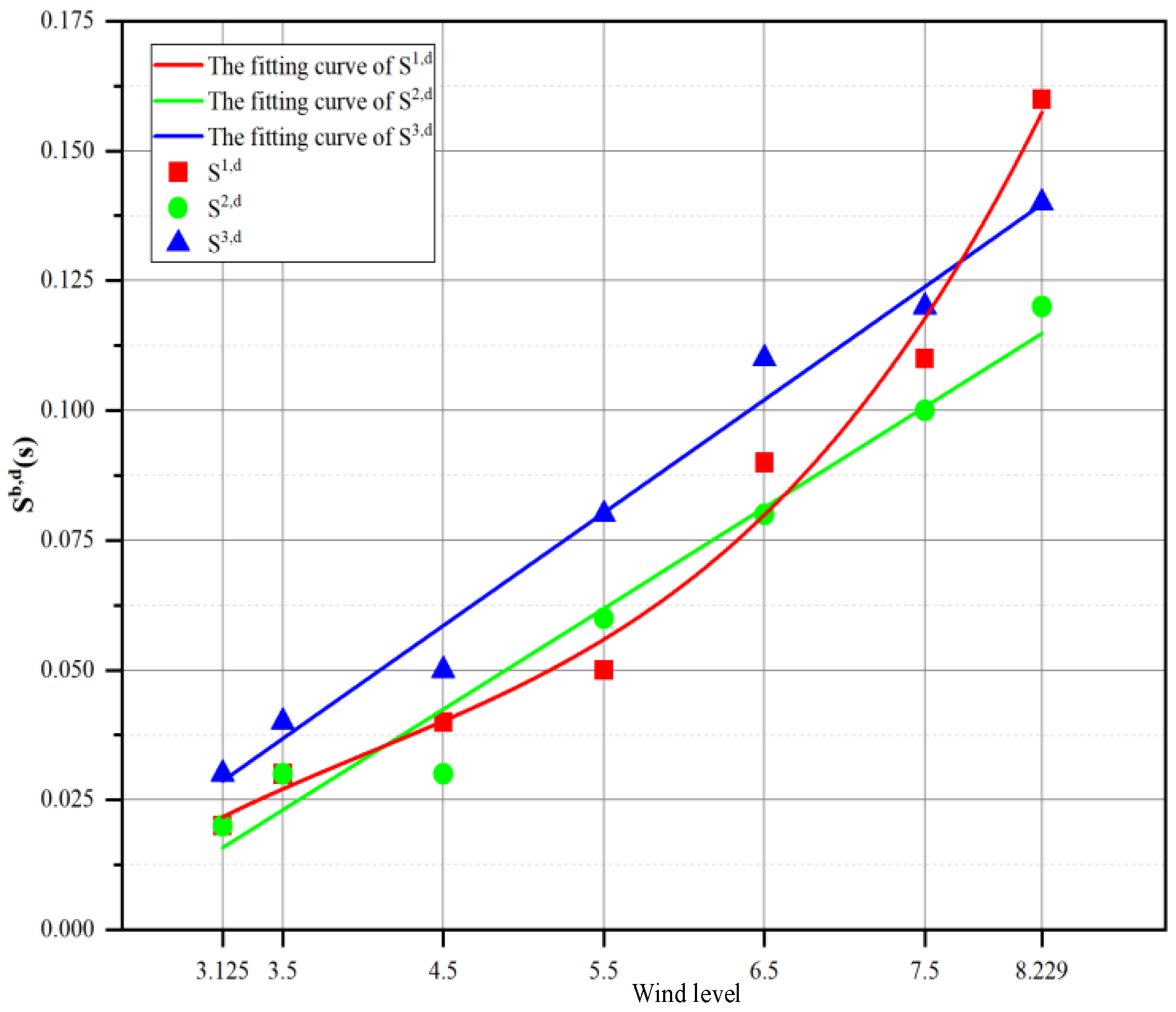
| Sb,d(s) | Wind Direction | ||||
|---|---|---|---|---|---|
| WNW | NW | NWN | Mean Value | ||
| Wind level | 3.125 | 0.02 | 0.02 | 0.03 | 0.02 |
| 3.5 | 0.03 | 0.03 | 0.04 | 0.03 | |
| 4.5 | 0.04 | 0.03 | 0.05 | 0.04 | |
| 5.5 | 0.05 | 0.06 | 0.08 | 0.06 | |
| 6.5 | 0.09 | 0.08 | 0.11 | 0.09 | |
| 7.5 | 0.11 | 0.10 | 0.12 | 0.11 | |
| 8.229 | 0.16 | 0.12 | 0.14 | 0.14 | |
Disclaimer/Publisher’s Note: The statements, opinions and data contained in all publications are solely those of the individual author(s) and contributor(s) and not of MDPI and/or the editor(s). MDPI and/or the editor(s) disclaim responsibility for any injury to people or property resulting from any ideas, methods, instructions or products referred to in the content. |
© 2025 by the authors. Licensee MDPI, Basel, Switzerland. This article is an open access article distributed under the terms and conditions of the Creative Commons Attribution (CC BY) license (https://creativecommons.org/licenses/by/4.0/).
Share and Cite
Huo, H.; Wang, Z.; Zhou, L.; Liu, Z.; Tu, M. Wind Field Simulation and Its Impacts on Athletes’ Performance, Based on the Computational Fluid Dynamics Method: A Case Study of the National Sliding Centre of the Beijing 2022 Winter Olympics. Appl. Sci. 2025, 15, 3685. https://doi.org/10.3390/app15073685
Huo H, Wang Z, Zhou L, Liu Z, Tu M. Wind Field Simulation and Its Impacts on Athletes’ Performance, Based on the Computational Fluid Dynamics Method: A Case Study of the National Sliding Centre of the Beijing 2022 Winter Olympics. Applied Sciences. 2025; 15(7):3685. https://doi.org/10.3390/app15073685
Chicago/Turabian StyleHuo, Hongyuan, Zhaofang Wang, Lingying Zhou, Zhansheng Liu, and Mincheng Tu. 2025. "Wind Field Simulation and Its Impacts on Athletes’ Performance, Based on the Computational Fluid Dynamics Method: A Case Study of the National Sliding Centre of the Beijing 2022 Winter Olympics" Applied Sciences 15, no. 7: 3685. https://doi.org/10.3390/app15073685
APA StyleHuo, H., Wang, Z., Zhou, L., Liu, Z., & Tu, M. (2025). Wind Field Simulation and Its Impacts on Athletes’ Performance, Based on the Computational Fluid Dynamics Method: A Case Study of the National Sliding Centre of the Beijing 2022 Winter Olympics. Applied Sciences, 15(7), 3685. https://doi.org/10.3390/app15073685