Assessing Voided Reinforced Concrete by Numerical Modelling of Impact-Generated Rayleigh Waves

Featured Application

This study highlights the potential of elastic wave-based testing, particularly Rayleigh wave (R-wave) methods, for the non-destructive evaluation of concrete structures. The developed computational approach can be applied to detect, localise, and characterise internal defects, such as voids, in concrete elements with only one-sided access. These findings can inform advanced methodologies in structural health monitoring, quality assurance during construction, and maintenance strategies for ageing infrastructure.

Abstract

Concrete structures require routine inspections. Within elastic wave-based non-destructive testing methods, the Rayleigh wave (R-wave)-based method shows great potential in defect characterisation with only one-side access required. This paper aims to investigate the effect of different locations and densities of voids on R-waves using a 2D finite element model. The numerical model was validated and calibrated with experimental results to increase the reliability and representativeness of the model developed. The difference between the R-wave velocity obtained from the numerical model and theory was within 5%, while the correlation between the R-wave waveform collected from the numerical and experimental data was 0.975. The developed numerical model was used to carry out a series of parametric studies investigating the relationship between different R-wave properties and void characteristics. The results revealed that the 5 kHz velocity index was the most sensitive for distributed void identification, with solid correlations up to 0.9879 reported. The correlations obtained from the data analysis suggest good feasibility of the demonstrated computational approach in evaluating the effect of defects in concrete on R-wave behaviour. This approach also offers useful insights into developing an alternative assessment methodology for internal damage localisation and characterisation utilising elastic wave measurements.

1. Introduction

It is of general interest to develop non-destructive inspection techniques, especially in Europe, where the building stock is relatively old. For example, across Europe, 60% of the non-residential buildings were built before 1980. In the UK specifically, over 50% of the residential building stock was built before 1960, while less than 15% was built between 1991 and 2010 (Artola, et al., 2016) [1]. Consequently, the development of non-destructive testing (NDT) methods and equipment have been accelerated to address the urgent need for either short-term or long-term inspections since NDT methods allow the inspection to be carried out without immobilising or damaging the structure (Lee, et al., 2014) [2], which makes them ideal for routine inspections.

Among the many NDT methods developed, elastic wave-based methods have great potential in detecting surface and subsurface defects. Other NDT methods, such as X-ray radiography and tomography, have limited practicability due to health and safety issues (Dwivedi, et al., 2018) [3]. Elastic wave-based methods are highly suitable for on-site inspections. Elastic waves are generated by an impact force striking onto a surface. Body waves (i.e., compression and shear waves) and surface waves (i.e., Rayleigh waves) are generated. Rayleigh waves (R-wave) make up the highest energy portion (67%) (Miller and Pursey, 1955) [4], which means that R-waves are easily excited and recorded at the surface. Also, an R-wave travels radially with a circular waveform. Compared to other waves (with spherical waveforms), the attenuation of the R-wave amplitude due to geometric spreading is much less than for body waves, making R-waves suitable for long-distance inspections (Hevin, et al., 1998) [5]. Surface waves are also preferred when structural members with restricted access need to be inspected, as only one-side access is required for surface wave-based methods.

The point-source/point-receiver pulse–echo technique was first proposed by Carino et al. (Carino, et al., 1986) [6] for flaw detection in concrete. This innovation initiated the development of impact–echo methods (Carino and Sansalone, 1992) [7]. At that time, only the detection of simple defects in concrete was demonstrated. Since then, many efforts have been made to evaluate the elastic wave-based methods for more complex conditions and more realistic scenarios, for example, the evaluation of concrete’s properties at early stages (Lefever, et al., 2020) [8], examination of concrete compressive strength (Ivanchev, 2018) [9], and characterisation of defects such as sub-surface cracks (Eraky, et al., 2018) [10] and honeycomb (Chai et al., 2016) [11]. Defect location, size, orientation and other characteristics can be determined from the information carried by the signal received.

During the early stages of development, wave propagation problems were studied either analytically or experimentally. The experimental approach is time-consuming and labour-intensive, which only allows limited cases to be studied. This is unfavourable due to the rapid increase in demand for the development of NDT methods. With the increase in computational ability and commercial software availability, numerical simulations with experimental model validation have become a popular combination. For example, in the evaluation of near-surface discontinuities, experiments monitor wave propagation on the surface, while numerical simulations provide details of vibration at any point within the body (Zerwer, et al., 2003) [12]. Understanding how a wave interacts with the defects is enhanced by the unparalleled insight provided by experiments and numerical simulations. Such understanding can later be utilised in the development of instrumentation design, experimental methodologies, and signal analysis schemes. Finite element modelling has been utilised to study various wave propagation problems in different materials. However, there is a limited number of papers addressing the heterogeneity inside concrete structures. For example, a wave propagates faster in high-density materials, and steel reinforcement will guide the wave. Different defects, such as cracks and voids, reflect, refract and scatter the propagating wave, which results in more complex wave behaviour.

R-wave-based detection methods are effective in the characterisation of near-surface defects. For defects located deeper under the surface, the method is limited by the R-wave propagation depth. This limitation of the method can be addressed by analysing the penetration depth of the R-wave. Numerical models help to simulate numerous combinations of parameters, such as wave frequency and defect properties. Thus, numerical models are helpful for investigating changes in R-wave properties against different defect characteristics. Correlations can be established by investigating the interaction between the wave and the defect, providing practical guidance on defect characterisation and further assessing the suitability of R-wave-based detection methods.

Current approaches to inspecting concrete structures through non-destructive methods struggle to identify internal voids correctly because these defects detrimentally affect structural stability. The existing ultrasonic testing technique for void characterisation requires specialised instrumentation because it fails to detect subtle void variations properly. This investigation fills the current research gap by studying the appropriate use of R-wave properties to characterise voided concrete in the form of low-density honeycombs. Specifically, the novelty of the work presented in this paper lies in the development of a simple yet practical 2D finite element model to simulate the propagation of R-waves in reinforced concrete that contains internal honeycombs, which are not often visible from the exterior. The numerical model was calibrated and validated with physical measurement data before being employed to study the influence of different honeycomb configurations on the propagation behaviour of R-waves derived from different excitation frequencies. An analysis of simulated wave data was carried out in the time and frequency domains, and simple correlations between R-wave velocity were developed to quantify changes with the density of honeycomb.

2. Simulation Model

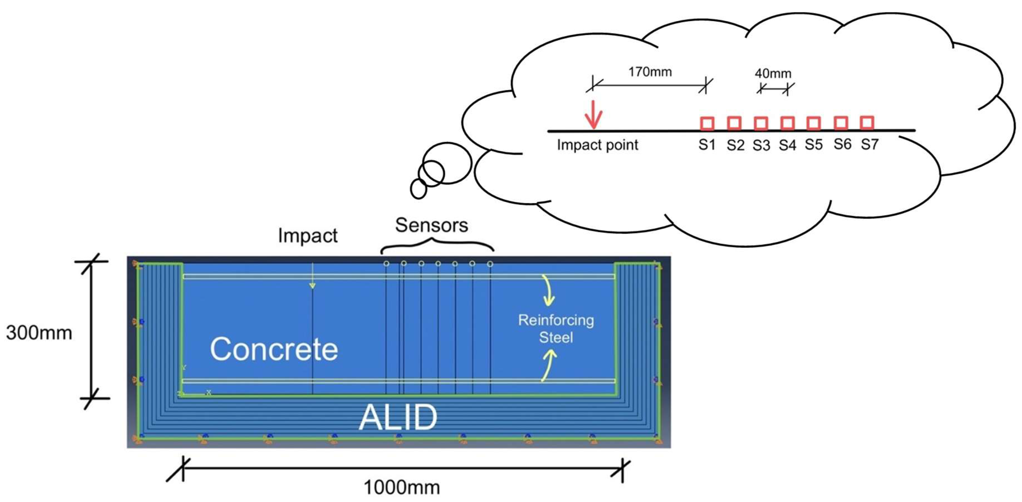
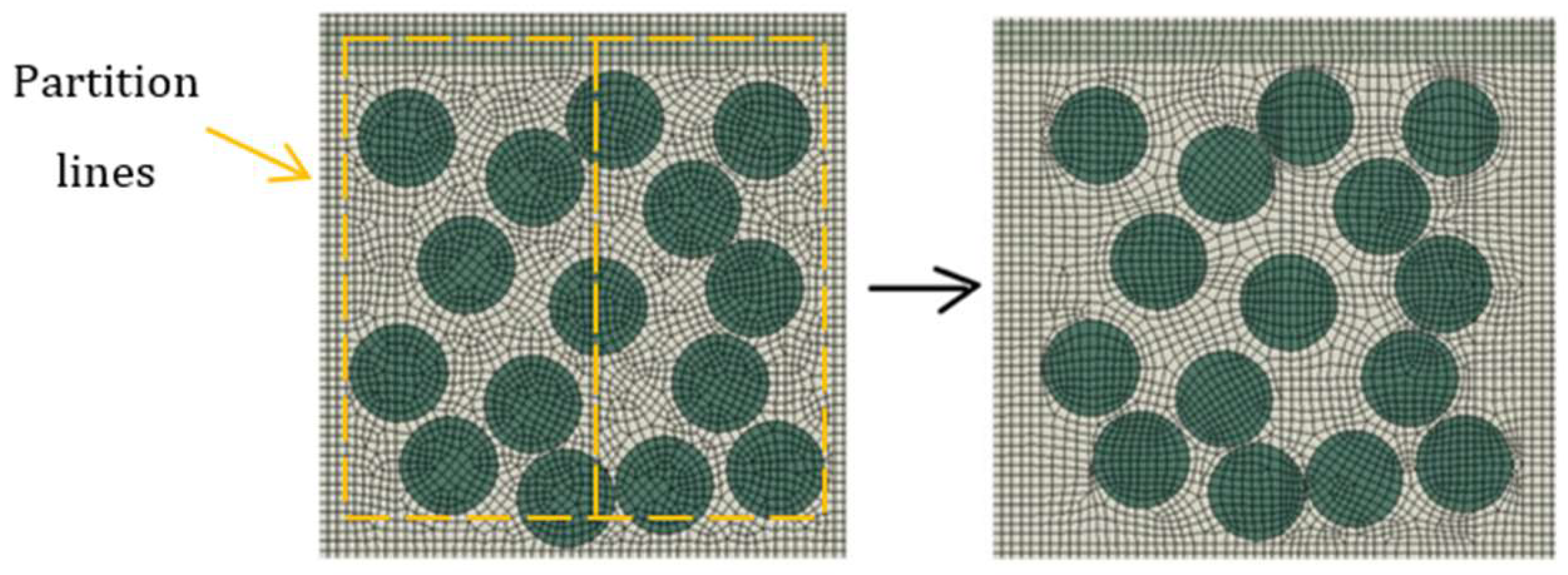
2.1. Reinforced Concrete Model

A 2D model was developed in this study. The model consisted of three parts: concrete, steel reinforcement, and boundary reflection absorbing layers for the reinforced concrete (RC) model. The dimensions of the reinforced/plain concrete region were 1000 mm × 300 mm (length × width). The steel reinforcement had a length of 1000 mm and a diameter of 10 mm. The concrete cover thickness was 30 mm. The mechanical properties of the concrete and steel reinforcement were configured as uniform throughout the whole study and produced longitudinal wave velocities of approximately 4300 m/s and 6099 m/s, for concrete and steel reinforcement, respectively, as reported in Lee et al., 2017 [13] for normal grade concrete. There were 10 layers of boundary reflection absorbing regions with increasing damping. The layers had a consistent thicknesses of 10 mm. The impact was defined by tabular amplitudes, in which the y coordinate is the amplitude of the impact wave, and the x coordinate is the time. The impact load was applied to a single node on the surface of the concrete. The sensors were arranged according to the experimental data acquisition layout to simplify the process of experimental validation (Lee, et al., 2017) [13]. There was a total of seven sensors. The distance between the first sensor and the impact point was 170 mm. There was a uniform spacing of 40 mm for the rest of the sensors. The impact sensor was placed at the centre of the concrete medium to reduce the contamination of the waveform by the boundary reflections. Due to the difference from the frequency range used in previous research (Lee, et al., 2017) [13], the sensor arrangement was checked against the ‘near-field’ effect in later stages. The configuration is shown in Figure 1.

This study used distributed voids in a concrete block to resemble honeycombs inside RC. The size and shape of honeycombs are highly variable in reality. The distributed voids were packed within a square block with dimensions of 100 × 100 mm. Then, the block was placed under the top reinforcement centre, and aligned with the very left, the middle or the very right sensor, as shown in Figure 2. The voids were randomly packed within the block with different densities using a MATLAB (R2020a) code (Semechko, 2018) [14]. The diameter of the voids was chosen for efficient packing, so the required modelling effort was minimised.

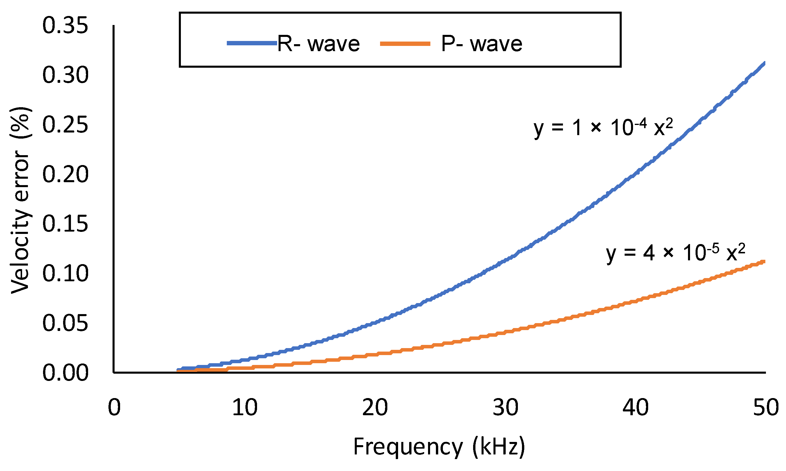
2.2. Element Type, Size and Wave Velocity

Both the concrete and steel were modelled as a 2D planar deformable shell structure. The selected element type was a 4-node, bi-linear plain strain element with reduced integration. There is a lesser number of integration points in an element with reduced integration. Thus, the element is more computationally economical to apply. However, a common problem with reducing integrated elements is the susceptibility to zero-energy mode, which produces unrealistic deformation (i.e., hourglassing) (SIMULIA, 2008) [15]. The ‘hourglass’ effect can be eliminated by either using very fine meshes or ABAQUS’s built-in hourglass control. In this study, ABAQUS’s built-in control was used.

The size of the mesh elements is directly linked to the accuracy of the model (Petyt, 1990) [16]. The size of the elements L_e is limited by the shortest wavelength λ_min of the waves applied to the model. The model is susceptible to spurious oscillations if the meshes are not fine enough (Bathe, 1996) [17]. Also, studies have shown that the velocity obtained from the numerical model will differ significantly from the actual velocity due to period elongation and amplitude decay (Bathe & Wilson, 1972) [18]. Therefore, very fine meshes are required to accommodate rapid spatial variation with high-frequency waves. The number of elements per wavelength N (i.e., mesh density) is suggested to be 20 to achieve good spatial resolution (Swanson Analysis Systems, 1992) [19], as shown in Equation (1).

$$L_e={\displaystyle \frac{{\lambda }_{min}}{\mathrm{N}}}={\displaystyle \frac{{\lambda }_{min}}{20}}$$

(1)

After several trials, the element size of the model was limited to 0.002 m to achieve optimised computing performance. The highest frequency f_max of the impact source adopted in this study was 50 kHz. The velocity of the R-wave, V_R, and P-wave components, VP, was taken as 2400 m/s and 4000 m/s. The values chosen fall within the range of typical velocities, i.e., between 1800 and 2500 m/s, and 3500 and 4500 m/s for R-wave and P-wave, respectively (Oh, 2007) [20].

Table 1. Calculated wavelengths and modal mesh densities and wavelengths.

fmax (kHz)	${\mathit{\lambda }}_{\mathit{R}}$(m)	NR	${\mathit{\lambda }}_{\mathit{P}}$(m)	NP
50	0.048	24	0.080	40

presents the calculated wavelengths (${\lambda }_R$ and ${\lambda }_P$) and mesh densities (N_R and N_P) for R-wave and P-wave, respectively.

The velocity error V_Err is related to the mesh density N by Equation (2) (Drozdz, 2008) [21], which is a function of the element size L_e, wave frequency f and wave velocity v. Figure 3 shows that adopting a wave frequency of 50 kHz, the velocity errors for the R-wave and P-wave components could reach a maximum of 0.313%, which is considered insignificant.

$$V_{Err}={\displaystyle \frac{180}{N^2}}={\displaystyle \frac{180}{{\left(\frac{\lambda }{L_e}\right)}^2}}={\displaystyle \frac{180{L_e}^2{\mathrm{f}}^2}{{\mathrm{v}}^2}}$$

(2)

The element’s aspect ratio is also critical. Quadrilateral elements were chosen in the modelling. The quadrilateral elements have better accuracies with the same node point arrangement as a triangular mesh (Petyt, 1990) [16]. The irregular meshing was avoided whenever possible in the modelling since any element distortion could possibly deteriorate the accuracy (Petyt, 1990) [16]. In this study, areas that required meshing were partitioned into regions with regular shapes to produce the best consistency in element sizing and distribution.

On the other hand, voids were modelled as “acoustic media” using a four-node linear 2D acoustic quadrilateral element with reduced integration. Distributed voids took the shape of circles and were randomly packed within the block, which created much distortion in the mesh. The elements around the voids were extremely irregular, which would drastically deteriorate the accuracy of the model if left unmodified. This study first tried partitioning the faces around the voids and applied a medial algorithm with the mesh control. An improvement in the mesh can be observed in Figure 4.

2.3. Explicit Simulation Time Control Parameters

In this study, a total wave simulation period of 0.001 s with a time step increment of 5 × 10⁻⁷ s was used. Demolding the explicit scheme is merely conditionally stable. The stability condition of the explicit modelling scheme was established by determining a suitable critical integration time step ${∆t}_{cr}$, known as the Courant–Friedrichs–Levy stability condition (Courant, et al., 1928) [22]. Using the simulated maximum wave frequency f_max of 50 kHz, ${∆t}_{cr}$ was obtained as 1 × 10⁻⁶ s using Equation (3) (Swanson Analysis Systems, 1992) [19].

$${∆t}_{cr}={\displaystyle \frac{1}{20f_{max}}}$$

(3)

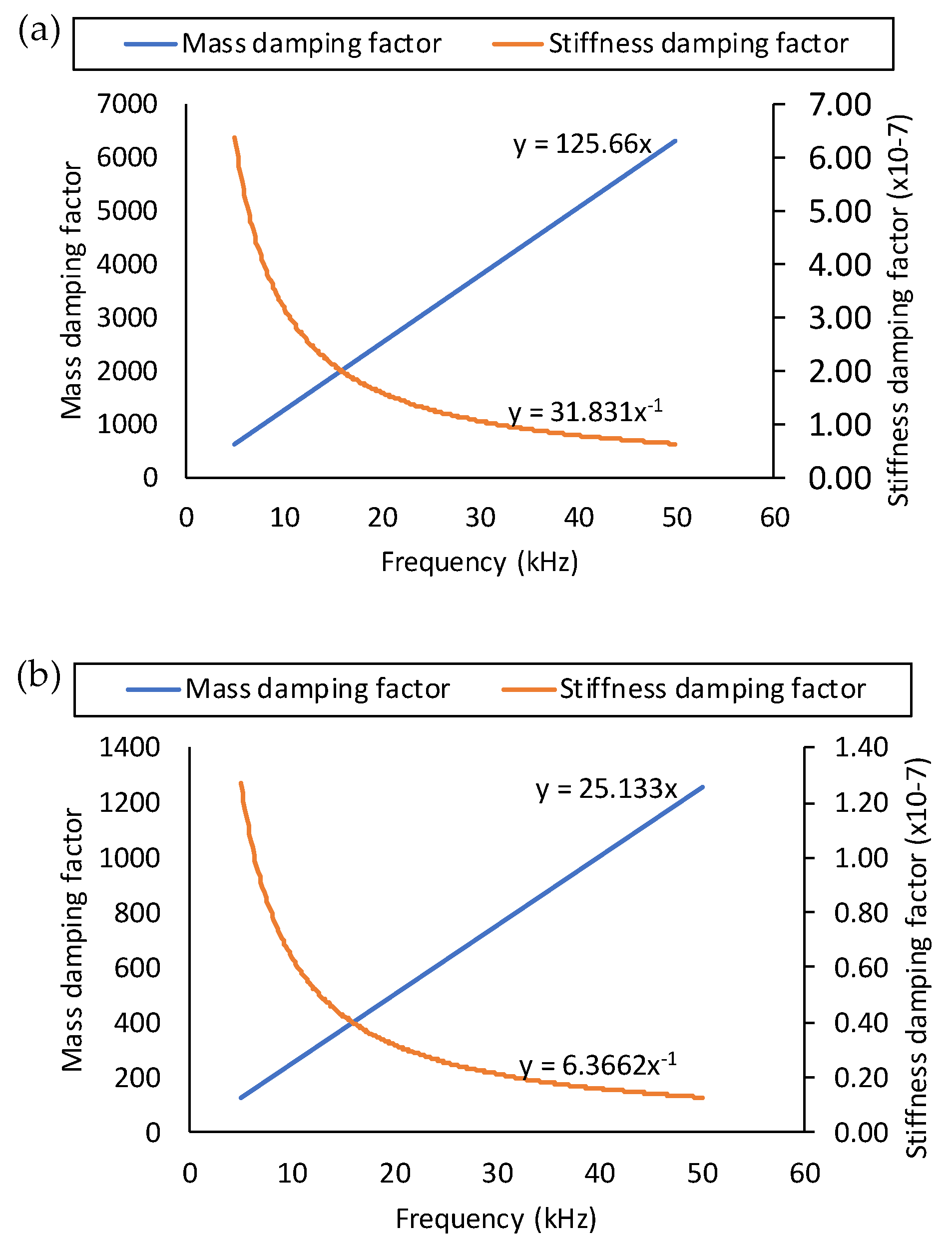
2.4. Material Properties and Damping Coefficients

The material properties needed to define a medium in wave propagation problems are the density, Young’s modulus, Poisson’s ratio and damping-related coefficients. The material properties are shown in

Table 2. Material properties.

Concrete Properties
Density (kg m−3)	2313
Young’s modulus (Pa)	28 × 109
Poisson’s ratio	0.2
Steel properties
Density (kg m−3)	7850
Young’s modulus (Pa)	200 × 109
Poisson’s ratio	0.3
Air properties
Density (kg m−3)	1.225
Bulk modulus (Pa)	142,000

.

For RC with small stress intensity (no void), the damping ratio for concrete, ξconcrete, is between 0.007 and 0.010. For steel reinforcement, the damping ratio, ξsteel, is between 0.001 and 0.002 (Mahrenholtz & Bachmann, 1995) [23]. Based on the values suggested, the initial damping ratios were assumed. Through further calibration with the experimental data, the final damping ratios used by the model were 0.010 for the concrete and 0.002 for the reinforcing steel. The mass and stiffness damping coefficients were calculated using Equations (4) and (5). The presence of angular frequency, ω, in the equations suggests that the damping depends on the wave frequency. The variations in the damping coefficients for concrete and steel are shown in Figure 5.

ξ = 1/2ω α → α = 2ωξ

(4)

ξ = 1/2 ωβ → β = 2ξ/ω

(5)

where α and β are the mass and stiffness damping coefficients, respectively.

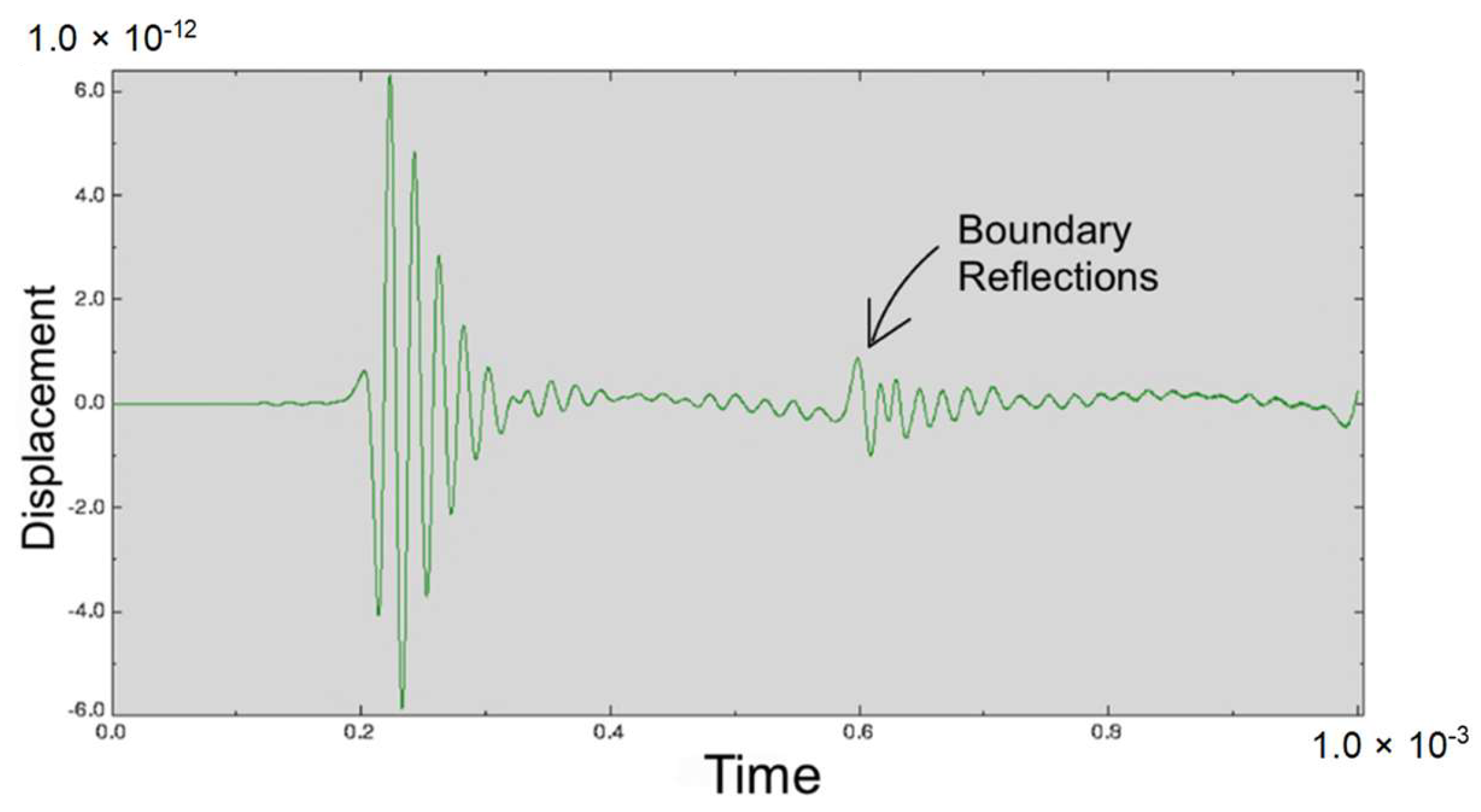
2.5. Model Boundary Conditions

The absorbing layer with increasing damping (ALID) method is employed in this paper to mitigate boundary reflections in numerical simulations of wave propagation. The presence of boundary reflections is confirmed to decrease the quality of a wavefield through significant wave energy scattering, making detection of a wave front and the subsequent wave components difficult and inaccurate. ALID restores the outgoing waves as they are in contact with the model boundaries through gradual absorption of wave energy. This helps to prevent waves from being reflected, scattered and “contaminating” the first arrivals of wave energies, which all lead to complications when extracting components of R-waves from simulated data. Within the context of this study, it is considered necessary to apply the ALID for optimising the modelling conditions so that direct wave propagation behaviour could be observed and evaluated effectively.

In terms of boundary condition setting, the numerical model was fixed at three edges: bottom face and the two side faces, leaving only the top face free to deform in the vertical direction. The ALID was applied to the three fixed edges of the concrete using 10 successive layers. The main parameter in ALID functions through the advancing mass damping coefficient α as it moves between the absorbing layers. The stiffness damping coefficient β receives a value of zero during damping layers to prevent efficiency reduction. The use of non-zero stiffness damping in absorption definition techniques leads to better results, as it enhances wave absorption and minimises artificial reflections at the interface between the absorbing layers and the concrete. However, this approach requires extremely short time increments, substantially increasing computational expenses. The damping layers share all the same attributes related to materials and mesh element characteristics and dimensions as the concrete model. This uniformity between the concrete and absorbing layers ensures that the material properties, mesh characteristics, and dimensions remain consistent, minimising impedance discrepancies. As a result, unwanted wave reflections at their interface are weakened, strengthening reflection attenuation. The gradual increase in the damping coefficient, α, can be obtained by Equation (6), as proposed by Rajagopal et al. (2012) [24], which was used in this study to define the smooth transition of wave propagation behaviour from the concrete model to the damping layers.

$$\alpha \left(x\right)={\alpha }_{max}X{\left(x\right)}^P$$

(6)

The value of X(x) varied from 0 to 1 (innermost layer to outermost layer). The value of P was set to be 3, as suggested by Mohseni & Ng (2018) [25]. In the calculation, the value of the maximum mass-damping coefficient ${\alpha }_{max}$ was taken as 2.5 × 10⁴.

On the other hand, the stiffness damping coefficients of the damping layers were all taken as zero. This was proposed by Drozdz (2008) [21] to avoid drastic losses in computational efficiency. Because the stiffness damping coefficients are much larger than the average value for general structures, especially towards the outer layers, very fine time increments are required, leading to an increase in computational time, making the method less economical. Except for the damping coefficients, all other properties of the damping layers were defined in the same way as those defined for the concrete model, including the material properties, mesh element type, and sizes. As exemplified by Figure 6, by replacing the infinite element with an absorbing boundary with increasing damping layers, boundary reflections have been effectively reduced to such an extent that they cause no significant contamination to the first-arriving wave groups.

3. Experimental Validation

3.1. Waveform Calibration

R-waves travel radially with a spherical waveform. They have been known to carry more energy than the body waves (primary and secondary waves), and the majority of the energy is concentrated near the surface of the medium that they propagate. This characteristic makes R-waves relatively easy to detect at the medium surface (Sansalone, et al., 1987) [26], and the change in their velocity and amplitudes are useful indicators that can be quantified against the change in the physical state of the medium through which they propagate. For transient waves, the R-wave arrival is often identified by locating either the first positive or negative waveform peak of the first-arriving wave packet. Therefore, a calibration of the waveform was carried out to obtain the best match between the first positive and negative peak amplitudes of the waves collected from experimental measurements and the numerical simulation, in which the elastic waves were generated on a plain concrete surface at a point 170 mm from the sensor. Details of the experimental measurements are reported elsewhere by the authors (Lee, et al., 2016) [27]. In the results analysis, the collected waveforms were normalised for amplitude against the highest positive peak for ease of comparison. Regression analysis and correlation analysis were then carried out to compare the experimental and the numerical waveforms. The superposed waveforms are shown in Figure 7. The coefficients obtained from the regression and correlation analyses are 0.950 and 0.975, indicating satisfactory calibration, which also validated the suitability of the afore-described waveform simulation configurations.

3.2. Wave Velocity

The theoretical velocities of the P-wave $V_P$ and R-wave components $V_R$ were calculated using Equations (7) and (8) (Jones, 1962) [28].

$$V_P=\sqrt{{\displaystyle \frac{\mathit{E}(1-\mathit{\upsilon })}{\mathit{\rho }(1+\mathit{\upsilon })(1-2\mathit{\upsilon })}}}$$

(7)

$$V_R={\displaystyle \frac{0.87+1.12\mathit{\upsilon }}{1+\mathit{\upsilon }}}\sqrt{{\displaystyle \frac{\mathit{E}}{\mathit{\rho }}}{\displaystyle \frac{1}{2(1+\mathit{\upsilon })}}}$$

(8)

The properties of the material used for the numerical model were substituted into the equations to compute the velocities.

Table 3. Comparisons of P- and R-wave velocities.

Theoretical	Concrete	Reinforcing Steel
$V_P(\mathrm{m}/\mathrm{s})$	3667	5856
$V_R$(m/s)	2047	2904
Experimental
$V_P(\mathrm{m}/\mathrm{s})$	4286	6099
$V_R(\mathrm{m}/\mathrm{s})$	2308	3220
Numerical
$V_P(\mathrm{m}/\mathrm{s})$	3940	5707
$V_R(\mathrm{m}/\mathrm{s})$	2000	2778

indicates the differences between the theoretical, experimental and numerical values.

The values obtained from the numerical model are closer to the theoretical predictions than to the experimental results, except for the P-wave velocity obtained from the plain concrete model. The differences in numerical results are within 10% when compared with the theoretical predictions and within 15% when compared with the experimental results. The main contributors to the discrepancies are considered to include limitations and variabilities associated with measuring the physical and mechanical properties of the materials in the laboratory. These influence the predictions of Young’s modulus, density and Poisson’s ratio of the materials modelled for the numerical simulations. In addition, there are potential uncertainties in the methods by which wave velocities were obtained experimentally. For example, these may include the existence of background noise that affects the signal-to-noise ratio and thus the accuracy of detected waveformsdamping and distortion of waves. Furthermore, the boundary reflection absorption layer applied in the numerical model may have also imposed unidentified computational uncertainties in simulating the propagation of waves.

4. Results of Simulations and Discussion

The numerical simulations were carried out considering cases with different combinations of wave frequency, distributed void density and defect location, as detailed in

Table 4. Simulation parameters.

Model	Defect Type	Wave Frequency (kHz)	Defective Area Density (% of Void)	Defect Depth from Surface (mm)	Defect Location
Sound RC	/	5, 25 and 50	/	/	/
Voided RC	Distributed Voids		10, 20, 40, 50, 100%	84	Between S1 and S3; S3 and S5; S5 and S7

. Altogether, there were 48 cases modelled and simulated, with results collected and analysed in the time and frequency domains to allow evaluation of elastic wave–void interactions and changes in R-wave velocity. This involves establishing the R-wave velocity index as an indicator used in the evaluation. Details of this are discussed in Section 4.4 below.

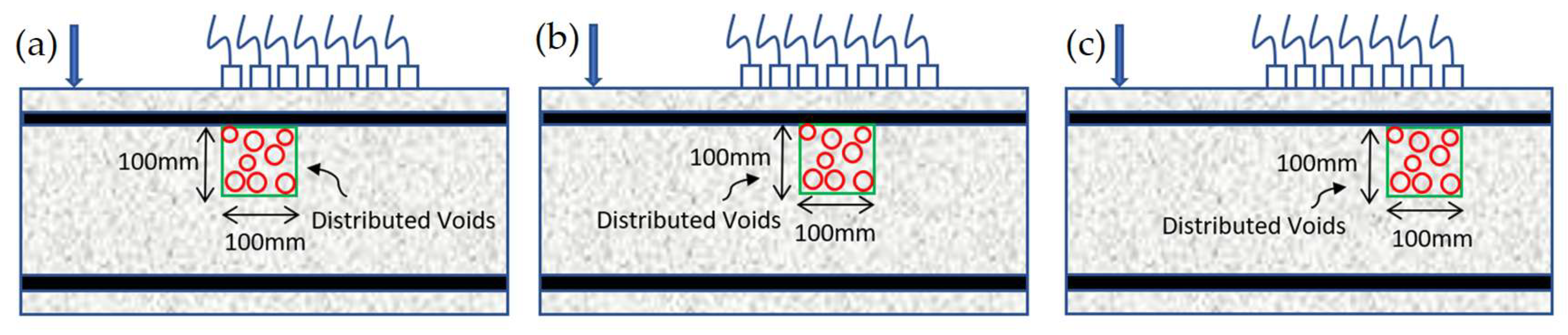
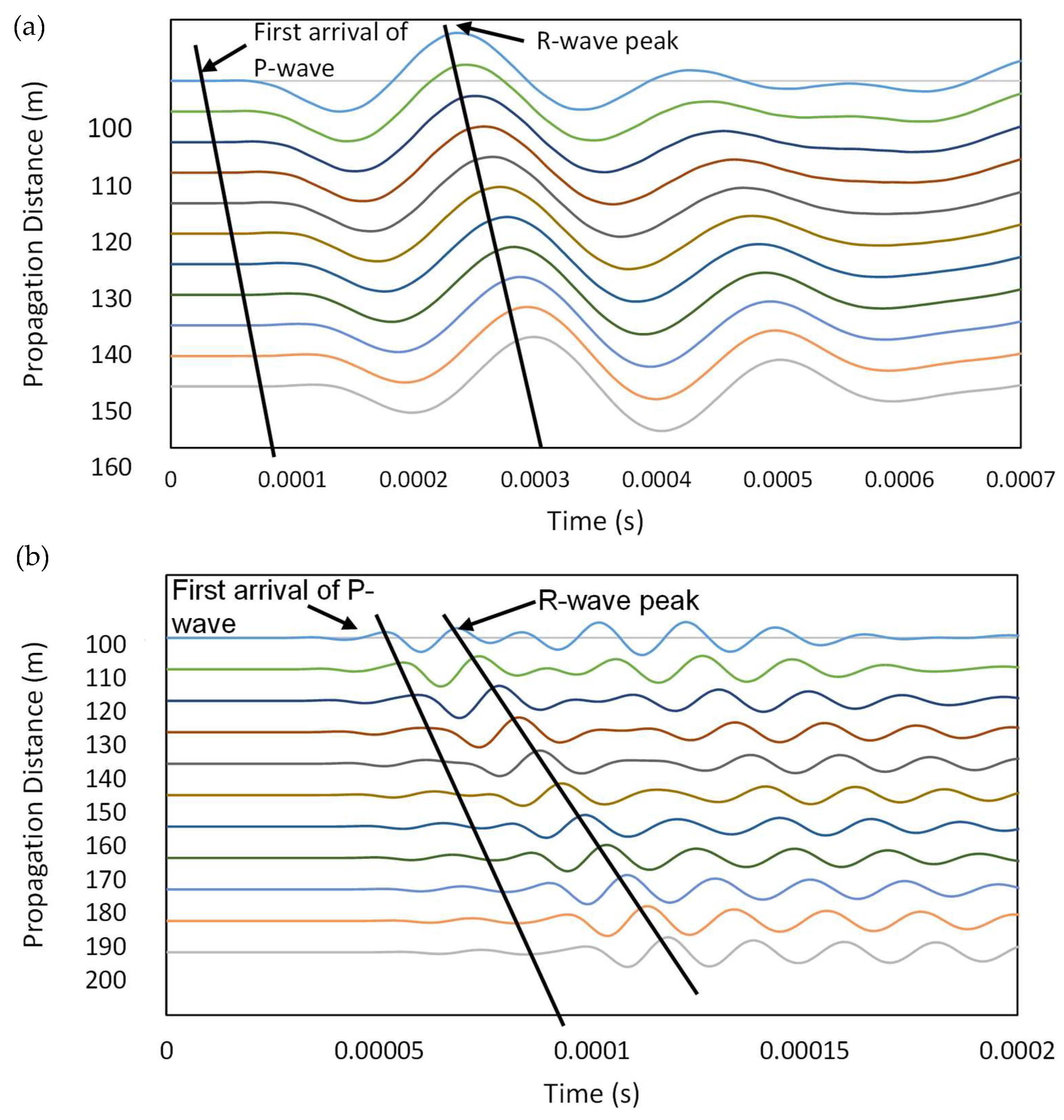
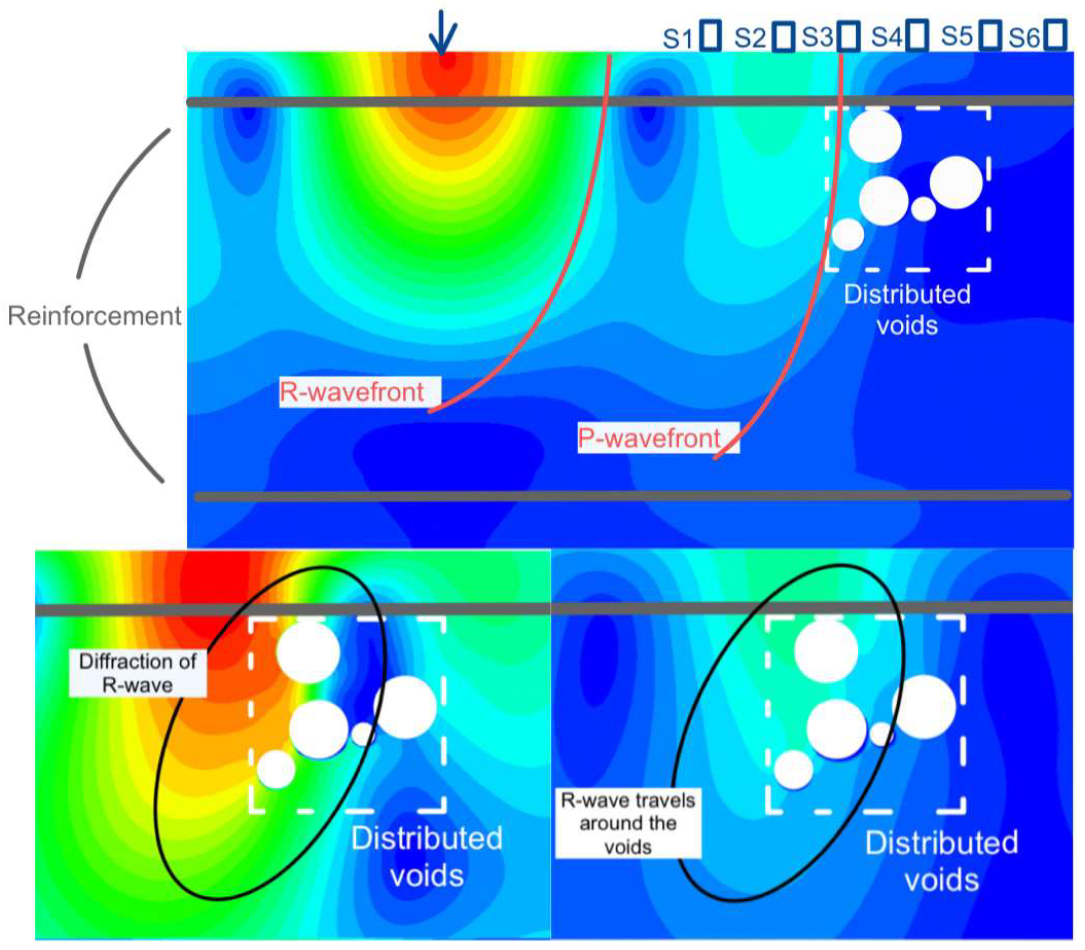
4.1. Near-Field Effect Study

When elastic wave excitation is located very close to the sensor position, there is a possibility that the R-wave component cannot be completely distinguished from the P- and S-waves in the detected waveform (Park, 2001) [29]. This phenomenon is widely termed the “near-field” effect. This can result in inaccurate velocity measurements of R-waves. To avoid erroneous measurements, a sufficient travel distance for R-waves must be allowed in the measurement. The recommended minimum spacing is 150 mm, as stated in Sansalone & Streett (1997) [30], which should work well with general types of impact elastic waves. Compiled from the results of the simulations conducted for this current study, Figure 8 shows some examples of waveform data collected at incremental propagation distances for 5 kHz and 50 kHz excitations. At 170 mm of wave travel distance, a clear separation between the first-arriving R-waves and the P-waves can be observed.

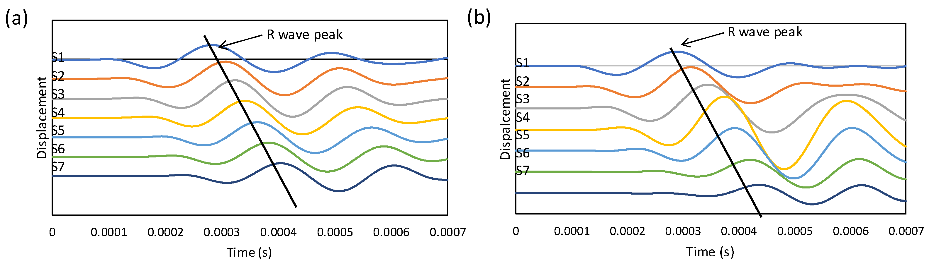
4.2. Time-Domain Data

Typical waveforms collected for 5 kHz and 50 kHz are shown in Figure 9. The first positive peak was identified as the R-wave. At 5 kHz, the wave amplitude decreased slightly from Sensor 4 to Sensor 7. With a 100% void, the amplitude was amplified at Sensor 4 and decreased afterwards. Delays in the R-wave peak became more pronounced with increasing void density.

When a wave passes through distributed voids, the voids act like obstacles, which increases the wave’s travel distance inside the voided block, resulting in delays in the wave. Also, the voids absorb and reflect portions of the wave energy. With distributed voids, the reflected waves are scattered within the voided block, whereas with a 100% void, the reflected wave travels back to the surface and converges with the propagating wave, resulting in the amplitude increase observed at Sensor 4. At Sensor 7, the wave energy is dissipated by different mechanisms, such as damping by the concrete, absorption, and scattering by the voids.

The wavefront of an R-wave is distorted when it encounters voids in its path. This distortion occurs due to diffraction, which occurs when the wave interacts with the boundaries (edges) of the void, particularly when the void size is comparable to the R-wave’s wavelength. In such cases, the wave bends around the void, rather than simply being blocked. Additionally, as the R-wave propagates through or around the void, scattering occurs, producing a complex wavefield behind it. This wavefield consists of multiple zones with varying amplitude strengths and phase relationships due to interference patterns. When multiple voids are present, dispersion takes place as the wave energy is redistributed in two ways: partial transmission through or around the empty space and reflection (which depend on the void’s size, shape, material properties), and the R-wave’s incidence angle.

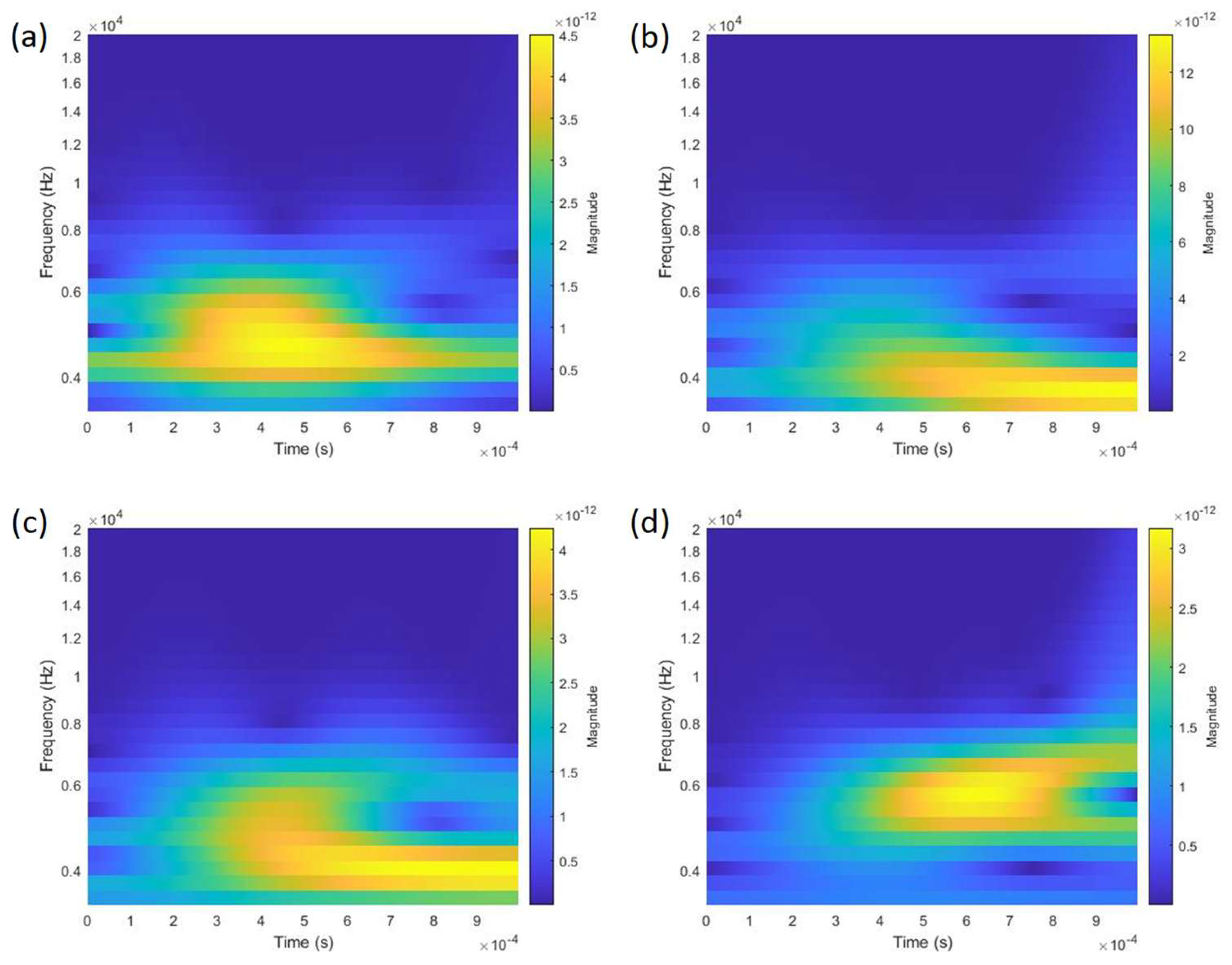
4.3. Frequency Domain Analysis

Continuous wavelet transform (CWT) was used to obtain the contour plots given in Figure 10. From the plots, the arrival of an R-wave peak is indicative of the occurrence of wave peak energy. Information on the frequency to which the peak wave energy belongs, as well as its magnitude and time of occurrence, can be extracted from the plots. From the findings, it is suggested that when void density increases (from 10% to 100%), a higher peak enethe data obtained by Sensor 7, which shows a lower peak energy magnitude. In addition, for Sensor 4, the recorded data indicate that the frequency corresponding to the peak energy (3.8 kHz) is lower than the dominant frequency of excitation (5 kHz). For Sensor 7, however, the recorded frequency becomes higher, approximately 5.9 kHz. It is also found that the delay in the arrival of peak wave energy is more pronounced at Sensor 4 when the void density increases. Multiple voids in the concrete create stronger wave scattering, which redistributes wave energy between the instrumented sensors. This leads to a further decrease in wave amplitude beyond the normal attenuation caused by propagation distance. The void boundaries also reflect waves, which interfere with incident waves and specifically increase amplitude readings at Sensor 4 when voids have a 100% density. The overall energy decay is influenced by changes in the energy dissipation mechanism, primarily due to material damping, scattering, and reflections—each varying based on wave frequency and void density. The frequency changes detected by Sensor 7 suggest modifications in the wave waveform patterns and associated resonant frequency behaviour. To better understand sensor–amplitude–frequency behaviour, future studies should provide precise descriptions of sensor positions relative to impact points and voids, as well as the effects of void density on wave paths.

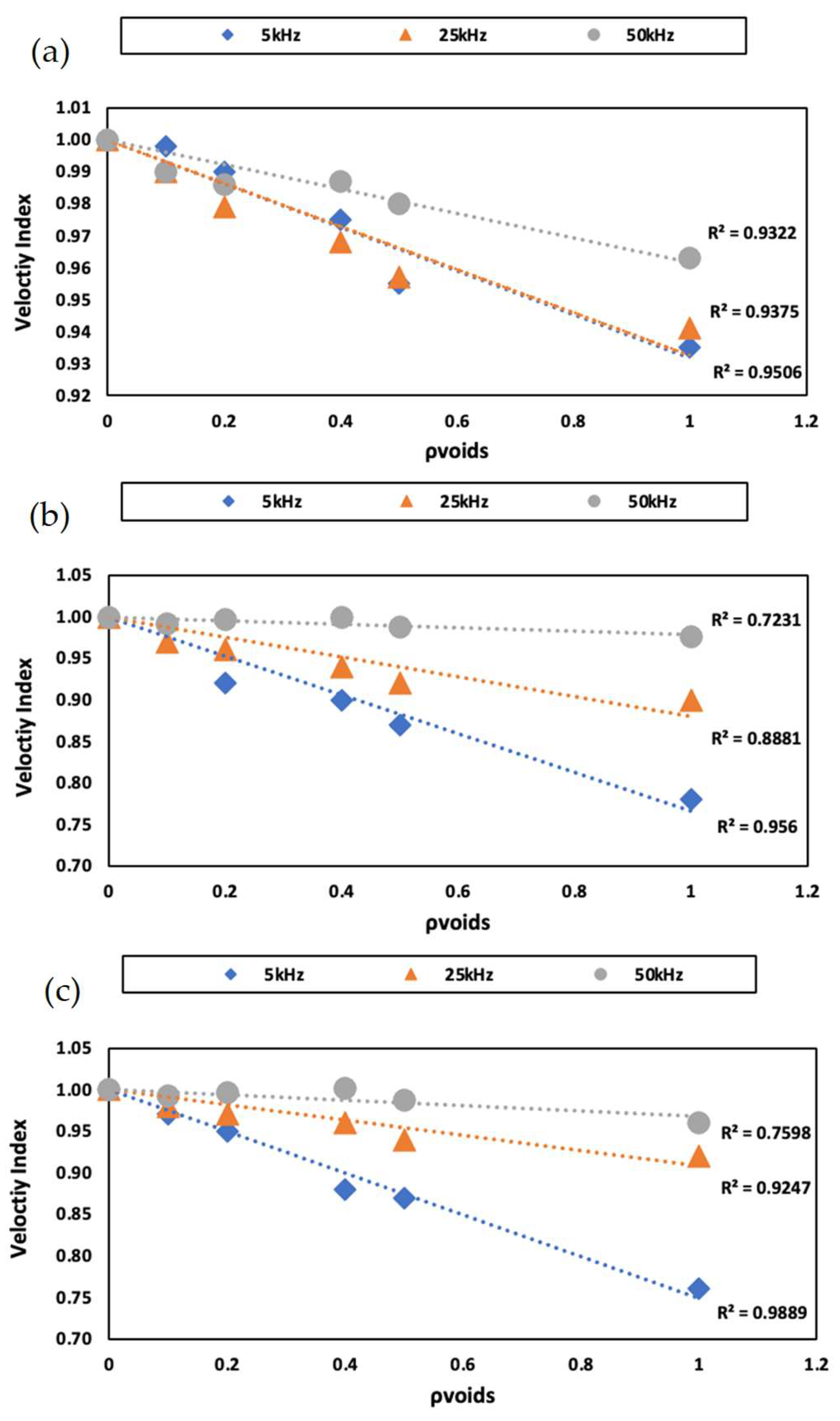
4.4. Correlation with Velocity Index

The velocity index, I_V is plotted against the density of voids in the concrete model, as shown in Figure 11, using the proposed formula given below.

$$I_V={\displaystyle \frac{V_{Defected}}{V_{Sound}}}$$

(9)

where V_Defected and V_Sound are the velocities of R-waves in the voided (defect) and unvoided (sound) models, respectively. Both V_Defected and V_Sound were obtained by calculating the gradient value of the linear regression for wave propagating distance versus propagation time plots, which is obtained by extracting the data acquired from each of the sensors for all the cases modelled and simulated. In general, the velocity index is found to decrease with void density, giving a good linear correlation in all cases covered in this study. For the cases of 5 kHz excitation frequency, the change in velocity index against void density is found to be more significant than that of the 50 kHz cases. This is most likely due to the longer wavelength given by the 5 kHz excitations, resulting in higher penetration depths of the R-waves and the waves being more easily distorted by voids.

In general, from the analysis of the numerical results, it can be confirmed that defects in concrete in the form of internal voids increase R-wave propagation time because of the resulting distortion. The analysis also revealed that waves excited with a dominant frequency of 50 kHz do not seem to be highly sensitive to the change in void density; this is evidenced by the velocity index results for all three void location cases, which barely change against void density, as opposed to those from the 5 kHz and 25 kHz cases, which show much more significant drops. Whilst it is widely agreed that the sensitivity of elastic waves against defects increases with their frequency, it is also commonly known that the R-wave penetration depth in any material is governed by wavelength in a positive correlation. This means that the penetration depth of R-waves normally decreases with an increase in their frequency. As confirmed from the simulation and analysis in this study, R-waves generated with a dominant frequency of 50 kHz could not propagate to the depth where the waves would be significantly distorted by a void. Additionally, it is known that R-wave amplitude decays exponentially with depth (Leiber, 2003) [31]. At the depth of the void block in the models studied herein, the simulated R-waves did not seem to possess sufficient energy to “interact” with the voids, and the sensors still detected them at the concrete surface.

As R-waves propagate in the concrete model, wave diffraction occurs as the waves reach the voided area. Energy is dissipated due to wave scattering and absorption by the medium, as visualised in the simulation exemplified in Figure 12. Reduced wave energy is apparent due to distortion generally, which also causes a delay in wave travel time. The key observations obtained from simulations, supported by the data analysis, confirm the contribution of the voided area to the reduction in R-wave velocity. The data analysis also suggests that the R-wave velocity index is a good indicator for estimating void density. The analysis suggests a promising potential for the velocity index to serve as an effective estimator for voided areas; however, in order to fully validate this assertion, it becomes necessary to delve deeper into understanding the various mechanisms contributing to the reduction in the R-wave velocity index. This would entail scrutinising potential correlations beyond linear relationships and exploring the influence of various environmental and structural factors on the velocity index. Such investigations are the basis of our next stage of study and are beyond the scope of the current paper. Furthermore, a meticulous study of disrupted waveforms obtained from different locations is required to gain a comprehensive understanding of the intricate interaction between R-waves and the void under a diverse range of configurations. Such in-depth analysis will offer valuable insights into quantifying the complex relationships and shed light on the multifaceted nature of the R-wave propagation phenomenon. Overall, the methodology for R-wave measurement and the related data analysis can be regarded as a feasible alternative approach for non-destructive assessment, enabling simple and quick concrete surface scanning with relatively straightforward instrumentation and data generation processes.

5. Feasibility of Modelling Framework

The testing method ensures a non-destructive approach, allowing multiple inspections of concrete structures without causing physical harm. A key advantage of this method is its ability to safely evaluate concrete structures in place. The examination reveals a correlation between void characteristics and Rayleigh wave property measurements at the 5 kHz velocity index. These correlations indicate that the method can both identify voids in concrete structures and determine their fundamental characteristics. The experimental system utilises basic equipment, enhancing its accessibility for field assessments compared to more complex testing methods. Additionally, the procedure relies on surface-based measurements, enabling rapid inspection of large concrete surfaces. The use of two-dimensional modelling improves computational efficiency, particularly during initial assessments or variable examination processes, compared to the complexity of full three-dimensional modelling.

6. Conclusions

This study demonstrated the feasibility of using a 2D finite element model to simulate impact-generated Rayleigh wave propagation in voided concrete. The model, calibrated and validated against experimental data, achieved strong agreement in waveform correlation (0.975 for plain concrete) and velocity (within 5% of theoretical values). While the correlation for reinforced concrete (0.567) was lower, it remains acceptable considering the model’s simplifications and ease of application for quick investigation. More crucially, we have identified the 5 kHz velocity index as a sensitive parameter for evaluating effects of void density on R-wave propagation, demonstrating a strong linear correlation. This insight signifies the potential of realising a simple in situ non-invasive measurement methodology for quantification and characterisation of concrete honeycomb. The suggested numerical modelling framework is relatively simple and easily applied, and does not require significant computation resources or highly specialised modelling skills. This framework could be adopted for rapid inspection for defects in reinforced concrete. Future work will focus on refining the model to improve the accuracy and effectiveness of damage detection in reinforced concrete and composite materials, aiming to achieve 3D simulations of materials with complex material configurations that are not fully isotropic. The data analysis scheme to be developed would also benefit from the incorporation of suitable machine learning algorithms for analysing the complex features of elastic waves. Machine learning could also assist with automating R-wave component extraction and wave property quantification and thus identifying the correlations of these properties with damage/defect characteristics.

References

1. Artola, I.; Rademaekers, K.; Williams, R.; Yearwood, J. Boosting Building Renovation: What Potential and Value for Europe; European Parliament: Brussels, Belgium, 2016. [Google Scholar]
2. Lee, F.W.; Chai, H.K.; Tan, T.H. Feasibility Study on Evaluating Surface Opening Cracks in Concrete by Multi-Channel Instrumented Surface Rayleigh Wave Propagation. Adv. Struct. Eng. 2014, 17, 785–799. [Google Scholar]
3. Dwivedi, S.K.; Vishwakarma, M.; Soni, A. Advances and researches on non destructive testing: A review. Mater. Today Proc. 2018, 5, 3690–3698. [Google Scholar] [CrossRef]
4. Miller, G.F.; Pursey, H. On the partition of energy between elastic waves in a semi-infinite solid. Proceeding R. Soc. 1955, 233, 55–69. [Google Scholar]
5. Hevin, G.; Abraham, O.; Pedersen, H.A.; Campillo, M. Characterisation of surface cracks with Rayleigh waves: A numerical model. NDT E Int. 1998, 31, 289–297. [Google Scholar]
6. Carino, N.J.; Sansalone, M.; Hsu, N.N. A point source point receiver pulse-echo technique for flaw detection in concrete. ACI J. Proc. 1986, 83, 199–208. [Google Scholar]
7. Carino, N.J.; Sansalone, M. Detection of voids in grouted ducts using the impact-echo method. ACI Mater. J. 1992, 89, 296–303. [Google Scholar]
8. Lefever, G.; Snoeck, D.; De Belie, N.; Van Vlierberghe, S.; Van Hemelrijck, D.; Aggelis, D.G. The contribution of elastic wave NDT to the characterisation of modern cementitious media. Sensors 2020, 20, 2959. [Google Scholar] [CrossRef] [PubMed]
9. Ivanchev, I. Experimental determination of concrete compressive strength by non-destructive ultrasonic pulse velocity method. Int. J. Res. Appl. Sci. Eng. Technol. 2018, 6, 2647–2651. [Google Scholar]
10. Eraky, A.; Samir, R.; El-Deeb, W.S.; Salama, A. Determination of Surface and Sub-Surface Cracks Location in Beams Using Rayleigh-Waves. Prog. Electromagn. Res. C 2018, 80, 233–247. [Google Scholar]
11. Chai, H.K.; Liu, K.F.; Behnia, A.; Yoshikazu, K.; Shiotani, T. Development of a tomography technique for assessment of the material condition of concrete using optimised elastic wave parameters. Materials 2016, 9, 291. [Google Scholar] [CrossRef] [PubMed]
12. Zerwer, A.; Polak, M.A.; Santamarina, J.C. Rayleigh Wave Propagation for the Detection of Near Surface Discontinuities: Finite Element Modeling. J. Non-Destr. Eval. 2003, 22, 39–52. [Google Scholar]
13. Lee, F.W.; Chai, H.K.; Lim, K.S. Characterising concrete surface notch using Rayleigh wave phase velocity and wavelet parametric analyses. Constr. Build. Mater. 2017, 136, 627–642. [Google Scholar]
14. Semechko, A. Fill Area with Random Circles Having Different Diameters. 2018. Available online: https://uk.mathworks.com/matlabcentral/answers/405186-fill-area-with-random-circles-having-different-diameters (accessed on 14 April 2021).
15. SIMULIA. Getting Started with Abaqus Intetactive Edition Version 6.8, s.l.; Dassault Systemes: Johnston, RI, USA, 2008. [Google Scholar]
16. Petyt, M. Forced response, I. In Introduction to Finite Element Vibration Analysis; Cambridge University Press: New York, NY, USA, 1990; pp. 386–449. [Google Scholar]
17. Bathe, K. Finite Element Procedures; Prentice Hall: Saddle River, NJ, USA, 1996. [Google Scholar]
18. Bathe, K.J.; Wilson, E.L. Stability and accuracy analysis of direct integration methods. Earthq. Eng. Struct. Dyn. 1972, 1, 283–291. [Google Scholar]
19. Swanson Analysis Systems. ANSYS User’s Manual for Revision 5.0; Swanson Analysis Systems: Houston, TX, USA, 1992. [Google Scholar]
20. Oh, T. Numerical Models Are Helpful in Simulating a Large Number of Combination of Parameters, Such as Wave Frequency and Defect Properties, to Aid the Process of Investigating the Change of Rayleigh Wave Properties Against Different Defect Characteristics; University of Illinois: Champaign, IL, USA, 2007. [Google Scholar]
21. Drozdz, M.B. Efficient Finite Element Modelling of Ultrasound Waves in Elastic Media; Imperial College London: London, UK, 2008. [Google Scholar]
22. Courant RFriedrichs, K.; Lewy, H. Über die partiellen Differenzengleichungen der mathematischen Physik. Math. Ann. 1928, 100, 32–74. [Google Scholar] [CrossRef]
23. Mahrenholtz, O.; Bachmann, H. Overall damping of a structure. In Vibration Problems in Structures Practical Guidelines Practical Guidelines; Birkäuser: Basel, Switzerland, 1995; pp. 166–168. [Google Scholar]
24. Rajagopal, P.; Drozdz, M.; Skelton, E.A.; Lowe, M.J.; Craster, R.V. On the use of absorbing layers to simulate the propagation of elastic waves in unbounded isotropic media using commercially available Finite Element packages. NDT E Int. 2012, 51, 30–40. [Google Scholar] [CrossRef]
25. Mohseni, H.; Ng, C.-T. Rayleigh wave propagation and scattering characteristics at debondings in fibre-reinforced polymer-retrofitted concrete structures. Struct. Health Monit. 2018, 18, 303–317. [Google Scholar]
26. Sansalone, M.; Carino, N.J.; Hsu, N.N. A Finite Element Study Transient Wave Propagation in Plates. J. Res. Natl. Bur. Stand. 1987, 92, 267–278. [Google Scholar]
27. Lee FW Lim, K.S.; Chai, H.K. Determination and extraction of Rayleigh-waves for concrete cracks characterisation based on matched filtering of center of energy. J. Sound Vib. 2016, 363, 303–315. [Google Scholar]
28. Jones, R. Non-Destructive Testing of Concrete; Cambridge University Press: London, UK, 1962. [Google Scholar]
29. Park, H.C. Development of a Microfluidic Mixer and Applications to Rapid Kinetic Studies of Calmodulin. Ph.D. Thesis, Korea Advanced Institute of Science and Technology, Daejeon, Republic of Kores, 2001. [Google Scholar]
30. Sansalone, M.J.; Streett, W.B. Impact-Echo; Bullbrier Press: Ithaca, NY, USA, 1997. [Google Scholar]
31. Leiber, C.-O.; Dobratz, B. Assessment of Safety and Risk with a Microscopic Model of Detonation; Elsevier: Amsterdam, The Netherlands, 2003; pp. 41–78. [Google Scholar]
Figure 1. Model configuration schematic.
Applsci 15 03635 g001
Figure 2. Distributed voids located below the sensor array at (a) left edge, (b) middle and (c) right edge of the latter.
Applsci 15 03635 g002
Figure 3. Velocity error caused by changing wave frequency.
Applsci 15 03635 g003
Figure 4. The meshing of distributed voids.
Applsci 15 03635 g004
Figure 5. Rayleigh damping coefficients, (a) concrete and (b) reinforced steel.
Applsci 15 03635 g005
Figure 6. Example of waveform data “recorded” by Sensor 7 with ALID implemented.
Applsci 15 03635 g006
Figure 7. Superposed waveforms (blue: experimental waveform; yellow: simulated waveform).
Applsci 15 03635 g007
Figure 8. Waveforms were collected for different propagation distances, with excitation frequencies of (a) 5 kHz and (b) 50 kHz.
Applsci 15 03635 g008
Figure 9. Stacked waterfall plots with an excitation frequency of 5 kHz for (a) 10% void and (b) 100% void models. Displacement is a normalised value.
Applsci 15 03635 g009
Figure 10. CWT plots for wave data with dominant excitation frequency of 5 kHz for (a) 10% and (b) 100% voided cases acquired at Sensor 4; and (c) 10% and (d) 100% voided cases acquired at Sensor 7.
Applsci 15 03635 g010
Figure 11. Velocity index versus void density for (a) left, (b) middle and (c) right cases.
Applsci 15 03635 g011
Figure 12. Simulation screenshots: wave propagation (top), diffraction of R-wave (bottom left), travel path of R-wave (bottom right).
Applsci 15 03635 g012