Abstract
Few-shot segmentation (FSS) aims to segment a query image with a few support images. However, there can be large differences between images from the same category, and similarities between different categories, making it a challenging task. In addition, most FSS methods use powerful encoders to extract features from the training class, which makes the model pay more attention to the features of the ‘seen’ class, and perform poorly on the segmentation task of ‘unseen’ classes. In this work, we propose a novel end-to-end model, called GFormer. GFormer has four components: encoder, prototype extractor, adversarial prototype generator, and decoder. Our encoder makes simple modifications to VIT to reduce the focus on image content, using a prototype extractor to extract prototype features from a range of support images. We further introduce different classes that are similar to the support image categories as negative examples, taking the support image categories as positive examples. We use the adversarial prototype generator to extract the adversarial prototypes from the positive and negative examples. The decoder segments the query images under the guidance of the prototypes. We conduct extensive experiments on a variety of unknown classes. The results verify the feasibility of the proposed model and prove that the proposed model has strong generalization performance for new classes.
1. Introduction
The traditional image semantic segmentation model needs a large number of samples with pixel-level annotation to train the model to obtain sufficient segmentation accuracy. However, due to the large labor cost of pixel-level annotation, the required samples are insufficient, which limits the scalability of image semantic segmentation. With the significant achievements in few-shot image classification, few-shot learning is gradually applied to semantic segmentation [1,2,3]. Few-shot learning uses a small amount of training data, and eliminates the need for labeling a large set of training images.
The fundamental idea of few-shot is how to effectively use the information provided by the labeled samples (called support) to segment the test (referred to as the query) image. The existing few-shot image segmentation methods usually adopt a double-branch structure—a support branch and a query branch—in which the support branch is used to realize the extraction of segmentation priors, and the query branch is used to complete the propagation of segmentation priors and obtain the segmentation results of query images. Early works used pretrained encoders as feature extractors, first obtaining the features of the support image and the query image, then extracting the semantic prototype from the features of the support images. Finally, pixels in the query feature map were matched by the support prototypes to obtain the segmentation results. However, the number of support prototypes was typically much less than the number of pixels in a query feature map, and there was information loss in extracting prototypes, which led to the limitation of segmentation performance. In order to solve these problems, Wang et al. [4] used the query image to reverse segment the support image with its prediction results to improve the semantic consistency of the prototype in the deep space. Liu and Qin [5] used the most significant category information in the query image to optimize the coarse initial prototype, improving the category perception ability of the prototype. MMFormer [6] used a class-agnostic segmenter to decompose the query image into multiple segment proposals, then merged the related segment proposals into the final mask guided by the support images. AAFormer [7] designed masked cross-attention to support pixel extraction of proxy tokens for foreground areas. Segmenter [8] captured the global image context and mapped it to pixel-level annotations by training learnable class embeddings. Inspired by Segmenter and AAFormer, we propose a prototype extractor, and consider directly training a learnable embedding to continuously acquire prototype features of specific regions in the image through cross-attention.
The differences between images from the same category and the similarities between different categories are the key obstacles to few-shot semantic segmentation, as shown in Figure 1. In order to solve the problem of differences between images from the same category, we generalize the proposed prototype extractor to a k-shot scene, which simultaneously obtains the prototype features of different images in the same category, and learns common features from them for containing more discriminative information. For the research to solve the similarities between different categories, most of the current methods use contrastive learning, which enhances the consistency and compactness of features through pixel-level contrastive learning. However, the comparison between pixels brings a huge amount of computation, and most of these methods rely on a large feature space, which requires prior information from the training samples to obtain better performance, and it is difficult to generalize to new classes that the model has not seen. Inspired by the idea of generative adversarial networks (GANs) [9], we believe that classes that have similarities to the target class can be regarded as fake samples generated by the generator, and we only need to implement the function of the discriminator to enable the model to distinguish between real/fake samples. In this paper, we propose an adversarial prototype generator, which refers to the support images as positive examples, and introduces different categories with similarities as negative examples. The module obtains the respective prototype features from the feature maps of positive and negative examples, and conducts a confrontation between positive and negative prototypes to make the final generated adversarial prototype focus on the positive features but not the negative examples, and obtains the feature differences between the positive and negative examples from the perspective of the prototype features. Inspired by SAM [10], we design a corresponding decoder, use cross-attention between feature prototypes and query image embedding, guide the segmentation of the query image through the interaction between them, and obtain more accurate segmentation results under the guidance of the adversarial prototype.
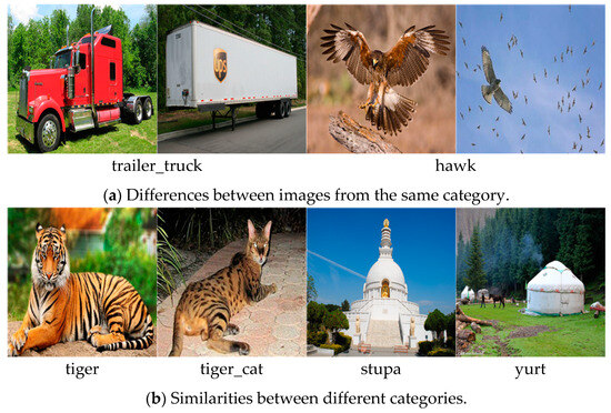
Figure 1.
Example of (a) differences between images from the same category and (b) similarities between different categories.
In addition, we note that, in most of the methods, the encoders used are complex and pretrained, and we assume that the encoder can capture features of any class. But, in fact, in the supervised learning settings, the pretrained encoder will focus more on the training class, will be less effective at extracting features from unknown classes, and may lead to overfitting. One solution to this problem is to make the model not memorize the semantic information learned during training, which is difficult to achieve with pretrained encoders. In our work, we reduce the emphasis on the feature extraction capabilities of the encoder, we make simple modifications to the encoder of Vision Transformer (ViT) [11], we remove some learnable parameters to reduce the encoder’s attention to the image content, and we make the model have better generalization performance for the new classes that are not trained.
Our main contributions are as follows:
- (1)
- We propose a novel few-shot semantic segmentation model. Specifically, we design a prototype extractor to obtain class-related prototype features, introduce positive and negative examples, design an adversarial prototype generator to learn the feature differences between positive and negative examples, and design a corresponding decoder to segment the query image under the guidance of prototype features.
- (2)
- We reduce the focus on feature extraction effects and make simple modifications to the encoder so that the model has better generalization performance for new classes.
- (3)
- A large number of experiments on the FSS-1000 dataset show that the proposed model has strong generalization ability for new classes, and the segmentation effect is not inferior to the FSS methods with the encoder.
2. Related Work
2.1. Semantic Segmentation
FCN was the first to use convolutional neural networks to realize semantic segmentation, and its encoder–decoder structure became the mainstream structure of semantic segmentation. In the follow-up work, for example, U-Net [12] uses skip connection to combine the encoded features and decoded features, which avoids the loss of information in the pooling process and enriches the spatial position information of the feature map. In order to expand the receptive field of convolution, the DeepLab series [13,14,15,16] proposed a dilated convolution to capture more complete contextual information, and proposed a dilated spatial pyramid pooling module to realize multiscale processing of images. Due to the restriction on local operations imposed by convolutions, it is difficult to establish dependencies over long distances. Some studies [17,18,19] applied transformer architecture for semantic segmentation, constructing global context relationships through attention mechanisms to achieve powerful segmentation performance. Since the transformer has global modeling capabilities, our work is carried out through the transformer architecture.
2.2. Few-Shot Semantic Segmentation
The task of few-shot semantic segmentation is to segment novel class query images with only a few labeled support images available. Existing FSS methods can be roughly categorized into two categories: prototype learning methods and meta-learning methods.
For prototypical learning, PL [20] is the first work introducing prototypical learning into few-shot segmentation, predicting foreground/background classes by comparing similarities with prototypes. PL constructed a prototype extractor based on the idea of classification, using global average pooling to extract discriminant semantic information. Wang et al. [4] further introduced a prototype alignment regularization to do bidirectional prototypical learning. Liu et al. [5] simultaneously captured segmentation cues from both support images and query images, and optimized the rough initial prototype with the most significant category information in the query image. MM-Former [6] added a feature alignment module before extracting prototypes to improve the effect of prototype matching.
For meta-learning, Shaban et al. [2] introduced meta-learning into few-shot semantic segmentation for the first time, using a weight hash layer to predict the weight of the query branch classifier. Amp [21] used multiscale information and normalized mask average pooling to generate guidance vectors, and fused historical guidance vectors through a smoothing adaptive scheme to construct the weights of the segmentation layer.
3. GFormer
3.1. Overview
Problem Definition. Widely used episodic meta-training [22] is adopted in few-shot segmentation. Specifically, we denote the training set as and testing set as , the categories of the two sets and are disjointed (). During training, we randomly select a set of sets from the training set; each set of images has the same category and is divided into a support set and a query set , where represents the number of support set images, and and are the images and their corresponding ground-truth binary mask. For each target category, we select an additional category from the training set that is similar to the target category, which is called the interference category. We name from the target category as the positive support set , and from the interference category as the negative support set . During testing, we perform the same for the test set. Note that both support masks and query masks are available for training, and only support mask is accessible during testing.
Model Architecture. As shown in Figure 2, the GFormer proposed in this paper has four components: encoder, prototype extractor, adversarial prototype generator, and decoder. Each module and training strategy will be described in detail next.
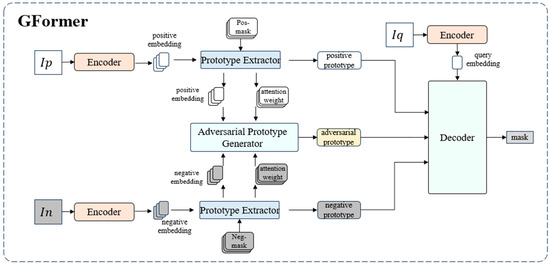
Figure 2.
The overview of the proposed GFormer. Each image goes through an encoder to obtain image embedding. The prototype extractor extracts the positive and negative prototypes from positive and negative image embeddings. The adversarial prototype generator generates the adversarial prototype. The decoder guides the segmentation of the query embedding through the joint action of multiple prototypes to obtain the final segmentation.
3.2. Encoder
Our encoders are built like VIT encoders, but there are two differences, as shown in Figure 3. (1) We do not use learnable positional embedding, rather we use sinusoidal positional embedding [23]. Compared with learnable positional embedding, sinusoidal positional coding does not need to be learned, which is suitable for the characteristics of small training data in few-shot semantic segmentation. Note that our position embedding is not directly added to the image embedding but is added to the query and key during the self-attention process, because the support image and the query image will go through the same encoder. If the position embedding is directly added, then the prototype feature will have position information in the process of prototype extraction, which will produce wrong guidance for the final segmentation. (2) At present, the mainstream relative position embedding adopts the contextual product method [24]. This kind of learnable relative position embedding is difficult to achieve the desired effect when the training sample is small. We propose a non-parameter relative position embedding , which is directly obtained according to the relative distance of image patches, calculated as:
where is the relative distance of image patches, is the relative distance between patch to image, and is the scale factor.
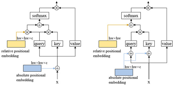
Figure 3.
The difference between the encoder of the original VIT (left) and the encoder in this paper (right).
The scale factor is used to control how much attention is paid to the surrounding patches.
3.3. Prototype Extractor
The module employs cross-attention in the transformer. The module has an inner learnable token, and receives the image and its corresponding binary mask as input.
Each layer performs three steps: (1) cross-attention from tokens (as queries) to masked image embedding, (2) cross-attention from the full image embedding (as queries) to tokens, and (3) MLP updates each token. Step (1): Inspiration is taken from AAFormer [7]. First, an attention weight matrix is calculated, and then the foreground part is preserved by masking. Formally:
Since there is no self-attention on the image, the module is able to ensure that only the information about the foreground of the image is obtained for each token update. The module uses the updated token as the prototype feature, denoted as . In addition, the attention matrix of step (1) and the updated image features of step (2) of each layer are retained for generating adversarial prototypes.
3.4. Adversarial Prototype Generator
The module design is shown in Figure 4. The module has an inner learnable token. After the positive and negative images pass through the prototype extractor, the updated image features and attention matrices are used as inputs for the adversarial prototype generator. Each layer has two branches: the enhancement branch and the suppression branch, which receive the positive and negative data, respectively. Different from the traditional method, we directly use the attention matrix from the prototype extractor to replace the query–key calculation, take the updated image features from the prototype extractor as the value, add the respective calculation results to the learnable token at the same time, and finally update the token with MLP. We take the updated token of the last layer as the adversarial prototype. After training, the adversarial prototype generated by the module can enhance the attention of the positive features and suppress the attention of the negative features.
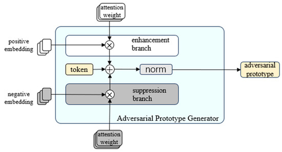
Figure 4.
Details of adversarial prototype generator.
3.5. Decoder
For the decoder, we take inspiration from SAM’s decoder and imitate its operation. We introduce learnable background class embedding to distinguish possible background regions. We concatenate the background class embedding and the positive prototype, naming them ‘tokens’. If negative support images are entered, the negative prototype and adversarial prototype are additionally inserted into the tokens. The decoder design is shown in Figure 5. Each decoder layer performs four steps: (1) self-attention on the tokens, (2) cross-attention from tokens (as queries) to the image embedding, (3) a point-wise MLP updates each token, and (4) cross-attention from the image embedding (as queries) to the tokens. After running the matcher, we follow the SAM [10] operation, upsample the updated image embedding, then pass the class prototype to the MLP, and finally predict the mask with a spatially pointwise product between the upscaled image embedding and the MLP’s output.
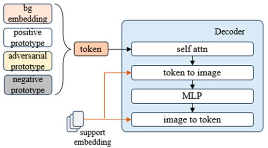
Figure 5.
Details of decoder.
3.6. Loss Function Definition
We calculate the losses for each module individually. We define as the predicted mask and as the ground truth. We supervise with focal loss. Formally:
where is the type of prototype, is image embeddings of image , is prototype.
Prototype Extractor. We use the same method as the prediction mask. We upsample the updated image embedding of the last layer of the module, pass the prototype to the MLP, and supervise the mask prediction for each image. The loss function can be formulated as:
where .
Adversarial Prototype Generator. For the adversarial prototype generator, we have two views: the enhancement view and the suppression view. In the enhancement view, we input positive and negative examples into the enhancement branch and suppression branch, respectively. Since the positive and query images are from the same category, the adversarial prototype obtained from this view can enhance the target category in the query image. In the suppression view, we input positive and negative examples into opposite branches; the resulting adversarial archetype will suppress the target category and treat it as the background. We use the adversarial prototypes from two views to calculate the masks at the same time. We concatenate the two masks and calculate the loss:
where is the enhancement view, is the suppression view, denotes the concatenate operation, is the background, and is the th support image.
Decoder. The final mask calculates the loss in the same way as the adversarial prototype generator; except, the final mask, for each layer, calculates the mask with the updated image embedding and positive prototype. The loss function can be formulated as:
3.7. Training Strategy
Due to the dependency between the inputs of the proposed prototype extractor, adversarial prototype generator, and decoder, we train the three components to a steady state in order, otherwise the model will not converge. Notice that, for the prototype extractor, we do not want the module to know any information related to the image content; therefore, in order to make it strictly follow the area instructions provided by the mask, we add the background mask to its training process, so that the prototype extractor can extract the background prototype under the guidance of the background mask.
4. Experiments
4.1. Dataset and Evaluation Metric
We conduct experiments on two popular few-shot segmentation benchmarks, FSS-1000 [25] and Pascal- [26]. FSS-1000 is a dataset dedicated to few-shot semantic segmentation that contains 1000 classes with 10 image–mask pairs for each class. Pascal-, with extra mask annotations SBD consisting of 20 classes, is separated into 4 splits. For each split, 15 classes are used for training and 5 classes for testing. We adopt mean intersection-over-union (mIoU) as the evaluation metrics for the experiments.
4.2. Implementation Details
We take the first 900 classes of the dataset as the training set and the last 100 classes as the test set. For the prototype extractor and the adversarial prototype generator, we randomly select 300 classes from the training set for training, 400 in decoder, and re-extract after the training of each module to ensure that the classes used by the 3 modules are not exactly the same; in this way, we ensure that the model will not be biased towards the training class, and will have a strong generalization ability for the new class. The input image size is 224 × 224, and the patch size is set to 8 × 8. All modules use the SGD optimizer and the Poly scheduler, whose power is 0.95, and use a Poly learning rate warmup for 5 epochs. For the prototype extractor, we train 100 epochs with a batch size of 1 and an initial learning rate of 5 × 10⁻⁴. For the adversarial prototype generator, we train 100 epochs, and, for each iteration, the batch size varies with a range of 3–9, with a cycle every 10 iterations, and an initial learning rate of 3 × 10⁻⁴. For the decoder, we train 300 epochs with a batch size of 1 and an initial learning rate of 3 × 10⁻⁴. The learning rate of the model is derived after many experiments. When greater than the set value, the model may not converge. Our method is implemented by PyTorch (version 1.13.1), and the graphics card used is an Nvidia GeForce 3060 (production location: China). Due to the limitation of experimental conditions, the number of layers of each module is reduced from 12 to 6.
4.3. Visualizations
In Figure 6, we compare the relative position coding effect of the proposed non-parameter relative position coding with the relative position coding in this paper by visualizing it, and the visualization diagram of the learnable coding is from the original image of this paper. The positional coding we propose implements a similar alternative to learnable positional encoding, where each patch focuses more on neighboring patches. The difference is that, as the number of layers increases, this phenomenon in this paper is attenuated by capturing enough local information, while the non-parameter positional encoding is constant, which may lead to reduced encoder performance. Although it is possible to achieve the same effect by adjusting the parameters, it is difficult, and our work is not focusing on this module.
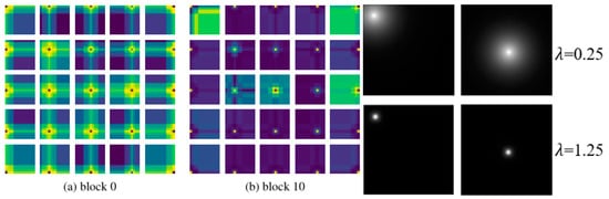
Figure 6.
The difference between relative position encoding in the contextual product method and non-parameter relative position encoding in this paper.
In Figure 7, we show the effect of the prototype extractor in the 1-shot and 5-shot scenes, respectively. They all belong to support images, and the token obtains the prototype features of the images under the guidance of the mask, and obtains the common prototype features of k support images at the same time in the k-shot scene.
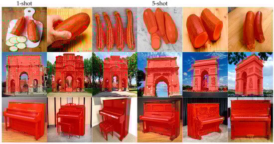
Figure 7.
The visualization of the activation effect of the prototype on the support images in 1-shot and 5-shot scenes.
In Figure 8a, we show the effects of the adversarial prototype generator. They all come from the support set, which means they do not go through the decoder. We put the positive example into the enhancement branch and the negative example into the suppression branch to obtain the positive adversarial prototype. We put the negative example into the enhancement branch and the positive example into the suppression branch to obtain the negative adversarial prototype. The positive adversarial archetype expands the distance between the foreground and the background to accurately find the pixels of the positive category, while the negative adversarial archetype suppresses the attention on the positive category and treats it as the background.
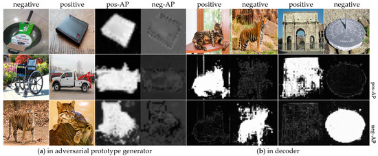
Figure 8.
The role of adversarial prototypes (APs) in helping the model distinguish between the two categories. We pick negative categories on the testing set based on the similarity of the prototypes, which may be completely different for humans but difficult for machines to distinguish.
Then, we show the effect of the decoder in Figure 8b. We stitch together the positive and negative query images, and use both the positive and negative adversarial prototypes to decode the stitched images. The results show that each adversarial prototype is able to find the category from the enhanced branch from the two images, and the category of the suppressed branch is regarded as the background. In Figure 9a, we show the final prediction for some of the unseen classes from FSS-1000. The results show that our model can correctly find the corresponding categories in the support images.
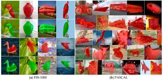
Figure 9.
Randomly sampled example 5-shot predictions on test images from FSS-1000 (a) and PASCAL- (b). Positive class prediction is overlaid in red; ground truth is overlaid in green.
4.4. Results
During the test, we found that the classes of some tiny objects could not be segmented correctly, especially the icon categories, and the prediction results were completely wrong. Therefore, we make the following analysis: for the icon categories in the image, they do not have much feature information in the channel dimension, and they can only be distinguished from the spatial dimension.
As can be seen in Figure 10, the pixels in the corresponding region of the truth value of this category are the same, the prototype features extracted from these images do not contain discriminative feature information, and the difference between different images in the channel dimension is only the color difference. Therefore, this type of category can only be discerned in terms of spatial dimensions. Since the feature extraction in the spatial dimension is not carried out in this work, it is difficult to correctly segment this type of category.
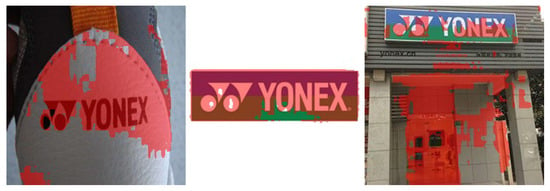
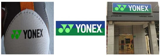
Figure 10.
Limitations on prototype extraction. Positive class prediction is overlaid in red. Ground truth is overlaid in green.
In Table 1, we present the experimental results of our method and other methods that test using FSS-1000.

Table 1.
mIoU scores on FSS-1000 test set of tasks for 1-shot and 5-learning.
According to the results, there is still a large gap between current performance and the method in FSS-1000. Since the focus of our work is on the generalization performance of the model rather than the accuracy of segmentation, we changed the learnable embedding in the original encoder to the non-parameter embedding. The reduction in segmentation accuracy brought by this operation was expected, which also indicates that our model has enormous potential for improvement.
For dataset FSS-1000, we used only 400 classes for training, while other papers used 760 classes. We did not use any data augmentation. In cases where the training data were significantly less than other works, we achieved similar segmentation performance. Therefore, our work has ‘strong’ generalization performance.
4.5. Result on Pascal-
We validated the generalization performance of the model on the Pascal- dataset. In order to make the results more convincing, we did not do any training on the Pascal- dataset but directly used the model trained on FSS-1000. In Table 2, we present the experimental results of our method and other methods that tested in Pascal-. We selected some images with large differences in shape and color from the Pascal- dataset for cross-validation, and the segmentation results are shown in Figure 9b. The results show that our model is able to extract prototypes from images with large intra-class differences, and can accurately identify the target class.
Table 2.
Comparison with other few-shot methods for 5-shot segmentation in Pascal-.
4.6. Ablation Study
In order to explore the impact of adversarial prototypes on model performance, we eliminated the adversarial prototype generator (APG) and retrained the model. In addition, we studied the effects of using only the positive adversarial prototype and using both positive and negative adversarial prototypes on segmentation performance. The results are shown in Table 3.
Table 3.
The effect of the adversarial prototype.
The experimental results show that the mIoU value obtained by the model with the adversarial prototype generator is about 4% higher than that of the model without the adversarial prototype generator. The performance improvement of adding a negative adversarial prototype to guide segmentation is not significant, the value has only increased by 0.35%. We make the following analysis: the positive adversarial archetype can increase the attention of positive examples, while the negative adversarial archetype inhibits the attention of positive examples. In the attention layer of the decoder, there is a huge gap between the attention of the foreground pixels in the query image to the two adversarial archetypes, and the negative adversarial archetypes play a small role in the attention weight. Therefore, the negative adversarial archetype will not have much effect on the segmentation of the positive example.
We performed ablation experiments on the encoder modifications, and the results are shown in Table 4.
Table 4.
The effect of our encoder.
The results show that the learnable position embedding will pay more attention to the training data, and the generalization performance of new classes will not be strong when the training data are less. The proposed encoder can effectively improve the generalization performance of new classes.
5. Discussion
This section discusses GFormer’s limitations.
- (1)
- The model is less effective at segmenting tiny objects. In this paper, the prototype feature extraction is only considered from the channel dimension. When the channel dimension of the image does not contain discriminative features, the model cannot achieve correct segmentation. One feasible approach is to extract the archetypal features of the image from the spatial dimension. However, in the course of the experiment, we found that the cross-attention convergence of the spatial dimension in the decoder is seriously difficult. In addition, it is difficult to extract adversarial archetypes in the spatial dimension. Therefore, prototype extraction technology in the spatial dimension is an important research direction for the future.
- (2)
- In this paper, the purpose of enhancing the generalization performance is achieved by using non-parametric positional encoding, but it sacrifices encoder performance. This also results in the final segmentation performance of the model being lower than some existing methods. How to achieve better generalization performance without reducing segmentation performance is the focus of future research work. In addition, due to experimental constraints, the number of layers of the model in this paper is less than that of other work, which may be one of the reasons for the poor segmentation performance. How to balance the number of model layers also needs to be studied.
6. Conclusions
In this paper, we propose a novel few-shot semantic segmentation model based on prototype learning. We design a prototype extractor to obtain prototype features, and introduce the concepts of positive and negative examples into the support images. We learn the adversarial prototype from them to enhance the target category in the image and suppress the interference category. We conduct extensive experiments on the new class, verifying the strong generalization ability of the proposed method for the new class. Our model has enormous potential for improvement, and provides a new idea for the study of few-shot semantic segmentation.
Author Contributions
Conceptualization, F.G.; methodology, F.G.; software, F.G.; validation, F.G.; formal analysis, F.G.; investigation, F.G. and D.Z.; resources, F.G. and D.Z.; data curation, F.G. and D.Z.; writing—original draft preparation, F.G.; writing—review and editing, F.G. and D.Z.; visualization, F.G.; supervision, F.G. and D.Z.; project administration, F.G. and D.Z.; funding acquisition, F.G. and D.Z. All authors have read and agreed to the published version of the manuscript.
Funding
This research received no external funding.
Institutional Review Board Statement
Not applicable.
Informed Consent Statement
Not applicable.
Data Availability Statement
The raw data supporting the conclusions of this article will be made available by the authors on request.
Conflicts of Interest
The authors declare no conflicts of interest.
References
- Nguyen, K.; Todorovic, S. Feature weighting and boosting for few-shot segmentation. In Proceedings of the IEEE/CVF International Conference on Computer Vision, Seoul, Republic of Korea, 27 October–2 November 2019; pp. 622–631. [Google Scholar]
- Shaban, A.; Bansal, S.; Liu, Z.; Essa, I.; Boots, B. One-shot learning for semantic segmentation. arXiv 2017, arXiv:1709.03410. [Google Scholar]
- Zhang, X.; Wei, Y.; Yang, Y.; Huang, T.S. Sg-one: Similarity guidance network for one-shot semantic segmentation. IEEE Trans. Cybern. 2020, 50, 3855–3865. [Google Scholar] [CrossRef] [PubMed]
- Wang, K.; Liew, J.H.; Zou, Y.; Zhou, D.; Feng, J. Panet: Few-shot image semantic segmentation with prototype alignment. In Proceedings of the IEEE/CVF International Conference on Computer Vision, Seoul, Republic of Korea, 27 October–2 November; pp. 9197–9206.
- Liu, J.; Qin, Y. Prototype refinement network for few-shot segmentation. arXiv 2020, arXiv:2002.03579. [Google Scholar]
- Zhang, G.; Navasardyan, S.; Chen, L.; Zhao, Y.; Wei, Y.; Shi, H. Mask matching transformer for few-shot segmentation. Adv. Neural Inf. Process. Syst. 2022, 35, 823–836. [Google Scholar]
- Wang, Y.; Sun, R.; Zhang, Z.; Zhang, T. Adaptive agent transformer for few-shot segmentation. In Proceedings of the European Conference on Computer Vision, Tel Aviv, Israel, 23–27 October 2022; Springer Nature: Cham, Switzerland; pp. 36–52. [Google Scholar]
- Strudel, R.; Garcia, R.; Laptev, I.; Schmid, C. Segmenter: Transformer for semantic segmentation. In Proceedings of the IEEE/CVF International Conference on Computer Vision, Montreal, BC, Canada, 11–17 October 2021; pp. 7262–7272. [Google Scholar]
- Goodfellow, I.; Pouget-Abadie, J.; Mirza, M.; Xu, B.; Warde-Farley, D.; Ozair, S.; Courville, A.; Bengio, Y. Generative adversarial networks. Commun. ACM 2020, 63, 139–144. [Google Scholar] [CrossRef]
- Kirillov, A.; Mintun, E.; Ravi, N.; Mao, H.; Rolland, C.; Gustafson, L.; Xiao, T.; Whitehead, S.; Berg, C.A.; Lo, W.-Y.; et al. Segment anything. In Proceedings of the IEEE/CVF International Conference on Computer Vision, Paris, France, 2–3 October 2023; pp. 4015–4026. [Google Scholar]
- Dosovitskiy, A.; Beyer, L.; Kolesnikov, A.; Weissenborn, D.; Zhai, X.; Unterthiner, T.; Dehghani, M.; Minderer, M.; Heigold, G.; Gelly, S.; et al. An image is worth 16x16 words: Transformers for image recognition at scale. In Proceedings of the 9th International Conference on Learning Representations, ICLR 2021, Virtual, 3–7 May 2021. [Google Scholar]
- Ronneberger, O.; Philipp, F.; Thomas, B. U-net: Convolutional networks for biomedical image segmentation. In Proceedings of the Medical Image Computing and Computer-Assisted Intervention–MICCAI 2015: 18th International Conference, Munich, Germany, 5–9 October 2015; Springer International Publishing: Cham, Switzerland, 2015. Part III 18. [Google Scholar]
- Chen, L.C.; Papandreou, G.; Kokkinos, I.; Murphy, K.; Yuille, A.L. Semantic image segmentation with deep convolutional nets and fully connected crfs. arXiv 2014, arXiv:1412.7062. [Google Scholar]
- Chen, L.C.; Papandreou, G.; Kokkinos, I.; Murphy, K.; Yuille, A.L. Deeplab: Semantic image segmentation with deep convolutional nets, atrous convolution, and fully connected crfs. IEEE Trans. Pattern Anal. Mach. Intell. 2017, 40, 834–848. [Google Scholar] [PubMed]
- Chen, L.C.; Papandreou, G.; Schroff, F.; Adam, H. Rethinking atrous convolution for semantic image segmentation. arXiv 2017, arXiv:1706.05587. [Google Scholar]
- Chen, L.C.; Zhu, Y.; Papandreou, G.; Schroff, F.; Adam, H. Encoder-decoder with atrous separable convolution for semantic image segmentation. In Proceedings of the European Conference on Computer Vision (ECCV), Munich, Germany, 8–14 September 2018; pp. 801–818. [Google Scholar]
- Cheng, B.; Schwing, A.; Kirillov, A. Per-pixel classification is not all you need for semantic segmentation. Adv. Neural Inf. Process. Syst. 2021, 34, 17864–17875. [Google Scholar]
- Cheng, B.; Misra, I.; Schwing, A.G.; Kirillov, A.; Girdhar, R. Masked-attention mask transformer for universal image segmentation. In Proceedings of the IEEE/CVF Conference on Computer Vision and Pattern Recognition, New Orleans, LA, USA, 18–24 June 2022; pp. 1290–1299. [Google Scholar]
- Xie, E.; Wang, W.; Yu, Z.; Anandkumar, A.; Alvarez, J.M.; Luo, P. SegFormer: Simple and efficient design for semantic segmentation with transformers. Adv. Neural Inf. Process. Syst. 2021, 34, 12077–12090. [Google Scholar]
- Dong, N.; Xing, E.P. Few-shot semantic segmentation with prototype learning. BMVC 2018, 3, 4. [Google Scholar]
- Siam, M.; Oreshkin, B.N.; Jagersand, M. Amp: Adaptive masked proxies for few-shot segmentation. In Proceedings of the IEEE/CVF International Conference on Computer Vision, Seoul, Republic of Korea, 27 October–2 November 2019; pp. 5249–5258. [Google Scholar]
- Vinyals, O.; Blundell, C.; Lillicrap, T.; Wierstra, D. Matching networks for one shot learning. Adv. Neural Inf. Process. Syst. 2016, 29. [Google Scholar]
- Vaswani, A. Attention is all you need. Adv. Neural Inf. Process. Syst. 2017, 30. [Google Scholar]
- Wu, K.; Peng, H.; Chen, M.; Fu, J.; Chao, H. Rethinking and improving relative position encoding for vision transformer. In Proceedings of the IEEE/CVF International Conference on Computer Vision, Montreal, BC, Canada, 11–17 October 2021. [Google Scholar]
- Li, X.; Wei, T.; Chen, Y.P.; Tai, Y.W.; Tang, C.K. Fss-1000: A 1000-class dataset for few-shot segmentation. In Proceedings of the IEEE/CVF Conference on Computer Vision and Pattern Recognition, Seattle, WA, USA, 14–19 June 2020; pp. 2869–2878. [Google Scholar]
- Everingham, M.; Gool, L.V.; Williams, C.K.I.; Winn, J.; Zisserman, A. The pascal visual object classes (voc) challenge. Int. J. Comput. Vis. 2010, 88, 303–338. [Google Scholar] [CrossRef]
- Rakelly, K.; Shelhamer, E.; Darrell, T.; Efros, A.A.; Levine, S. Few-shot segmentation propagation with guided networks. arXiv 2018, arXiv:1806.07373. [Google Scholar]
- Hendryx, S.M.; Leach, A.B.; Hein, P.D.; Morrison, C.T. Meta-learning initializations for image segmentation. arXiv 2019, arXiv:1912.06290. [Google Scholar]
- Zhang, C.; Lin, G.; Liu, F.; Yao, R.; Shen, C. Canet: Class-agnostic segmentation networks with iterative refinement and attentive few-shot learning. In Proceedings of the IEEE/CVF Conference on Computer Vision and Pattern Recognition, Long Beach, CA, USA, 15–20 June 2019; pp. 5217–5226. [Google Scholar]
- Lu, Z.; He, S.; Zhu, X.; Zhang, L.; Song, Y.Z.; Xiang, T. Simpler is better: Few-shot semantic segmentation with classifier weight transformer. In Proceedings of the IEEE/CVF International Conference on Computer Vision, Montreal, BC, Canada, 11–17 October; pp. 8741–8750.
Disclaimer/Publisher’s Note: The statements, opinions and data contained in all publications are solely those of the individual author(s) and contributor(s) and not of MDPI and/or the editor(s). MDPI and/or the editor(s) disclaim responsibility for any injury to people or property resulting from any ideas, methods, instructions or products referred to in the content. |
© 2025 by the authors. Licensee MDPI, Basel, Switzerland. This article is an open access article distributed under the terms and conditions of the Creative Commons Attribution (CC BY) license (https://creativecommons.org/licenses/by/4.0/).