Research on Offshore Vessel Trajectory Prediction Based on PSO-CNN-RGRU-Attention

Abstract

In busy offshore waters with high vessel density and intersecting shipping lanes, the risk of collisions and accidents is significantly increased. To address the problem of insufficient feature extraction capability of traditional recurrent neural networks (RNNs) in ship trajectory prediction in busy nearshore areas, this paper proposes a hybrid model based on Particle Swarm Optimization (PSO), Convolutional Neural Networks (CNN), Residual Networks, Attention Mechanism, and Gated Recurrent Units (GRU), named PSO-CNN-RGRU-Attention, for ship trajectory prediction. This study utilizes real Automatic Identification System (AIS) data and applies the PSO algorithm to optimize the model and determine the optimal parameters, using a sliding window method for input and output prediction. The effectiveness and practicality of the model have been fully verified. Experimental results show that, compared to the PSO-CNN-GRU model, the proposed model improves the longitude by 7.8%, 3.4%, and 1.7% in terms of Mean Absolute Error (MAE), Mean Squared Error (MSE), and Root Mean Squared Error (RMSE), respectively, and improves the latitude by 48.3%, 62.9%, and 39.2%, respectively. This has significantly contributed to enhancing the safety of ship navigation in the Bohai Strait.

1. Introduction

With the rapid rise of the offshore economy and the widespread application of the Automatic Identification System (AIS) in offshore areas, the offshore shipping industry has become an indispensable link in increased trade activities and regional economies, significantly promoting economic prosperity in offshore regions. The increasing number of vessels due to growing or unintentional trade has led to a sharp rise in navigation risks. Therefore, to enhance navigational safety, Tu et al. [1] focused on the development of intelligent collision avoidance technologies for vessels. The prerequisite for achieving this goal is a deep understanding of vessel movement trajectories. As a result, many scholars have shifted their research focus to the field of vessel trajectory prediction, aiming to accurately predict the future paths of vessels through scientific methods and models, thereby effectively avoiding collision risks.

Scholars from around the world have explored and proposed diverse vessel trajectory prediction methods based on traditional prediction algorithms. Specifically, an approach has innovatively combined the Grey Prediction Method with the Hidden Markov Model [2]. It first utilizes the Grey Prediction Method to fit the original vessel trajectory and weakens the randomness and time variability in the trajectory by calculating the absolute ratio sequence. Subsequently, the Hidden Markov Model is introduced for more accurate trajectory predictions. In contrast, Mazzarella et al. [3] designed a Bayesian prediction model based on a particle filter, grounded in traffic route knowledge. This model has demonstrated excellent performance in experiments conducted in specific strait areas. However, the application scope of this model has certain limitations; it is primarily suitable for inland waterways or fixed channel environments and may perform poorly under the complex navigation conditions of open waters.

To address the limitations of traditional prediction methods in handling nonlinear vessel trajectories—such as poor performance, large output fluctuations, and a lack of self-learning, organization, and adaptability—vessel trajectory prediction technologies based on deep learning models have gradually become a research hotspot. Researchers have innovatively combined the unique trajectory features of vessels with time series data and applied neural networks in deep learning, especially the Long Short-Term Memory (LSTM) [4,5,6,7] model, to predict the operating trajectories of vessels. The Gated Recurrent Unit (GRU) [8] model has been applied to vessel trajectory prediction. Compared with the LSTM model, the GRU model can quickly learn and process data without significantly sacrificing prediction accuracy, thus improving the training speed. This approach has significantly enhanced prediction accuracy. However, in some complex scenarios, a single model still faces the challenge of insufficient prediction accuracy. Bidirectional Long Short-Term Memory (Bi-LSTM) [9] and Bidirectional Gated Recurrent Unit (Bi-GRU) [10] neural networks have been respectively introduced into the field of vessel trajectory prediction. This innovative initiative has significantly enhanced the performance of prediction models. Through a bidirectional design, these two models can simultaneously capture features in time series data from both past and future directions, thereby achieving a more comprehensive understanding of the complex relationships between data points. Composite neural network models such as CNN-GRU [11], MP-LSTM [12], TCN-Bi-LSTM [13], and RNN-Bi-LSTM [14] have been proposed and applied in the field of vessel trajectory prediction. Compared to single neural networks, these composite models exhibit significant advantages in learning capability. By integrating the characteristics of different neural network architectures, they achieve a deeper and more comprehensive understanding and modelling of vessel trajectory data. While composite neural networks have stronger learning capabilities than single neural networks, they come with complex network structures, large computational demands, and the challenge of determining the hyperparameters of the network model.

Existing hyperparameter optimization methods, such as manual search, grid search, and random search, generally suffer from issues like high blindness and the tendency to fall into local optima. As a result, heuristic algorithms like Particle Swarm Optimization (PSO) have gradually become the preferred approach for optimizing network model hyperparameters for researchers both domestically and internationally. The PSO [15] algorithm has been used to optimize the LSTM neural network. By analyzing input data statistics and the performance of hidden units, the model predicted the closing price of the Indian Energy Exchange with minimal error, providing an efficient solution for electricity price forecasting. The Sparrow Search Algorithm (SSA) [16] has been applied to optimize the GRU model, utilizing data decomposition to obtain feature components. Combining actual company data, they compared various models to provide a better solution for short-term load forecasting in the power grid. The Artificial Bee Colony (ABC) [17] algorithm has been used to optimize the LSTM and construct a hybrid model. Based on a big data platform to compute sentiment polarity indices, the model was used to analyze and predict stock data, significantly improving the accuracy of stock market predictions through multi-model comparisons. The Whale Optimization Algorithm (WOA) [18] has been employed to optimize the LSTM model. The linear components of air pollution data were first extracted and the nonlinear components were output. WOA was then used to search for LSTM hyperparameters. Ultimately, the model predicted air pollutant data and was compared with several related models, providing more accurate reference data for pollutant concentration prediction in air pollution control.

In this context, this paper focuses on the important and complex task of vessel trajectory prediction, addressing the challenges associated with determining hyperparameters in existing models and the limitations encountered when processing time series data, particularly the insufficient capture of long-term dependencies and limited generalization capabilities. We propose an optimization scheme for a CNN-RGRU-Attention [19] fusion model based on the Particle Swarm Optimization algorithm to enhance the accuracy of vessel trajectory prediction. The model integrates CNN for extracting local features, residual connections to alleviate gradient vanishing, max pooling for downsampling, and fully connected layers for dimensionality reduction. Additionally, it introduces an attention mechanism to enhance sensitivity to key information while the dual-layer GRU captures long-term dependencies, improving prediction accuracy and the model’s generalization ability.

2. Related Works

Before delving into the construction of the offshore vessel trajectory prediction model based on PSO-CNN-RGRU-Attention, it is necessary to systematically review the basic theoretical knowledge underlying this model. In this section, the core principles of the Convolutional Neural Network (CNN), Gated Recurrent Unit (GRU), and Attention Module will be expounded upon in sequence.

2.1. CNN Residual Module

Convolutional Neural Networks (CNN) [20], as a special form of feedforward neural network, can be divided into two main modules: feature extraction and classification. The feature extraction module cleverly integrates multiple convolutional layers and pooling layers. Through the sliding computation of convolution kernels on the data and the downsampling mechanism of pooling layers, it effectively mines and abstracts the deep features within the data. Given the unique advantages of one-dimensional CNNs in processing time series data, this paper specifically selects this architecture to handle the latitude and longitude time series data of vessels.

The input data for a one-dimensional CNN is a one-dimensional array, and the convolution process involves the sliding of the convolution kernel along the one-dimensional axis. Figure 1 shows an example with a convolution kernel size of three, one convolutional layer, and a stride of one, where X₁, X₂, and X₃ represent the input data, and Y₁ represents the output feature vector.

As the depth of neural networks increases, the capability for feature extraction becomes richer, indicating that neural networks possess stronger nonlinear representation abilities. However, experiments have shown that increasing the number of network layers often leads to performance degradation. He et al. [21] highlighted the issues of gradient vanishing, gradient explosion, and model degradation that can arise from blindly stacking convolutional layers and pooling layers when proposing the residual network.

This paper introduces a residual module, and the operation process of this module is as follows: The input data first enters the first one-dimensional convolutional layer. The convolutional kernels slide over the data and perform multiplication and addition operations to extract preliminary features. These preliminary features then enter the second one-dimensional convolutional layer, where the convolutional kernels further dig into the data to obtain more abstract features. Subsequently, the abstract features are added element-wise to the preliminary features, integrating the information from both the high-level and low-level features, which helps prevent the vanishing gradient problem. The results of the addition go through an activation function to introduce non-linearity, and finally, the final output is generated. This approach allows the network to learn the mapping relationship between input and output more effectively, overcoming issues such as gradient vanishing and further optimizing network performance. The structure is shown in Figure 2. If the input of the i-th residual block is denoted as Xⁱ and the output as Xⁱ⁺¹, the relationship between them is as follows:

$$X^{i+1}=Activation(X^i+F\left(X^i\right))$$

(1)

In Equation (1), Activation refers to the activation function, and F(Xⁱ) represents the operations of the residual module.

2.2. GRU Model

The Gated Recurrent Unit (GRU) [22] is an improved version of the Long Short-Term Memory (LSTM) neural network and is currently a mainstream architecture for time series prediction. Compared to LSTM, the GRU network has a simpler structure, offering higher training speed and computational efficiency. Figure 3 illustrates the unit structure of the GRU, which consists of a reset gate r_t and an update gate z_t. The output h_t is determined by the current input x_t and the previous state h_t−1. The output calculation formulas for the GRU unit are shown in Equations (2)–(5).

$$r_t=\sigma \left(W_r{x}_t+U_r{h}_{t-1}+b_r\right)$$

(2)

$$z_t=\sigma \left(W_z{x}_t+U_z{h}_{t-1}+b_z\right)$$

(3)

$$H_t=\tanh \left(W_h{x}_t+U_h\left(r_t·h_{t-1}\right)+b_h\right)$$

(4)

$$h_t=\left(1-z_t\right)·h_{t-1}+z_t·H_t$$

(5)

In this context, b_r, b_z, and b_h are the bias vectors for the input x_t and the previous state h_t−1; W_r, W_z, W_h, U_r, U_z, and U_h are the weight matrices; $\sigma$ represents the sigmoid function; and tanh refers to the hyperbolic tangent function. The structure of the GRU unit is shown in Figure 3.

2.3. Attention Layer

The Attention Mechanism [23] is a commonly used technique in computer science and machine learning, designed to make models more accurate and efficient when processing sequence data. In traditional neural networks, the output of each neuron relies solely on the outputs of all neurons in the previous layer. In contrast, the attention mechanism allows the output of each neuron to be influenced not only by the outputs of all neurons in the previous layer, but also to be weighted according to different parts of the input data, assigning different weights to different parts.

The specific details are shown in Figure 4. A method is chosen to calculate the similarity between the query and each key, resulting in a similarity score for each key that matches the dimension of the value. The similarity scores are normalized using the softmax function to obtain the attention weights for each key-value pair. By multiplying the attention weights by the corresponding value for each key and then summing them up, we obtain the final output. Here, a represents the inertia weight, s denotes the attention score, and * represents the multiplication operation between the weight value and the corresponding Value. The attention aggregation function f is expressed as a weighted sum of values in Equation (6), where the attention weight between the query $q$ and $k_i$ is calculated by mapping the two vectors into a scalar through Equation (6), and then running softmax to obtain Equation (7).

$$f\left(q,\left(k_1,v_1\right),\dots ,\left(k_m,v_m\right)\right)=\sum _{i=1}^m a\left(q,k_i\right)v_i\in R^V$$

(6)

$$a\left(q,k_i\right)=softmax\left(a\left(q,k_i\right)\right)={\displaystyle \frac{\mathit{exp}\left(a\left(q,k_i\right)\right)}{{\sum }_{j=1}^m\mathit{exp}\left(a\left(q,k_j\right)\right)}}\in R$$

(7)

2.4. PSO-CNN-RGRU-Attention Trajectory Prediction Model

Particle Swarm Optimization (PSO) is a type of swarm intelligence optimization algorithm in the field of artificial intelligence. The PSO algorithm initially initializes a group of particles in the solution space. Each particle has three attributes: velocity, position, and fitness value, with each particle representing a potential optimal solution to an extremum optimization problem. Velocity indicates the speed of the particle’s movement, position represents the direction of movement, and the fitness value is calculated by the fitness function. The Mean Square Error (MSE) between the predicted values and the true values is calculated using Equation (8), where $y_i$ represents the true value of the sample, ${\widehat{y}}_i$ represents the predicted value of the sample, and N represents the number of samples in the sequence. In this paper, the fitness function is given by Equation (9), which records the fitness value, the individual extremum P_best, and the global extremum G_best positions.

$$MSE={\displaystyle \frac{1}{N}}\sum _{i=1}^N {\left(y_i-{\widehat{y}}_i\right)}^2$$

(8)

$$Fit\left(x\right)=min\left(MSE\right)$$

(9)

Based on the analysis of the performance of CNN, residual modules, attention mechanisms, and GRU, a new model is proposed that integrates CNN residual modules, attention mechanisms, and GRU. For the input AIS data, the model first uses CNN layers for preliminary feature extraction. In this process, the output of the first convolutional layer is added to the output of the second convolutional layer via a residual connection. This helps alleviate the vanishing gradient problem and simplifies network training. Next, an attention mechanism is introduced, enabling the model to dynamically focus on the important parts of the sequence. By using the attention mechanism, the model can adjust the weights based on the importance of each time step in the sequence, thereby highlighting critical information. Finally, the data with attention weights are fed into the GRU layer, which further models the sequential data and outputs the representation of the sequence. The output is passed through a fully connected layer to generate the final prediction result. The PSO optimization algorithm is used to optimize the learning rate and the number of neurons in the model, yielding the best hyperparameters. The structure of the model is shown in Figure 5.

The PSO-CNN-RGRU-Attention regression problem is essentially a task of ship trajectory prediction. Generally, a ship’s navigation state follows a certain pattern over a period of time. The navigation states at past and current moments significantly influence the navigation state at the next moment. Therefore, by inputting the ship’s navigation information at both past and current times, the model can output the future trajectory data in terms of longitude and latitude. The network is trained using real ship trajectory samples to establish a corresponding mapping relationship between the input and output, enabling the prediction of the ship’s future trajectory.

3. Methods

3.1. Data Selection and Preprocessing

The experimental data in this paper comes from the Bohai Strait in China, collected on 4 August 2022. The longitude range was from 37°52′48′′ to 38°52′48′′, and the latitude range was from 120°0′0′′ to 122°0′0′′. This area is a vital shipping region in China, and studying ship trajectories in this region holds significant importance for ensuring navigation safety and related matters.

The data parsed from the original AIS messages often contain errors, making it impossible to use the raw AIS data directly. Forcing the use of the original AIS data would result in experimental outcomes that do not align with actual conditions. The AIS data used in this paper includes six pieces of information: the Maritime Mobile Service Identity (MMSI) of the vessel, the time the AIS message was sent, the vessel’s longitude information, the vessel’s latitude information, the vessel’s speed over ground, and the vessel’s heading information. Following the IEC61162-1 [24] international standard, the AIS data was processed, and the AIS data preprocessing module consisted of the following four steps:

Step 1: Anomaly Detection. Data anomalies include the following obvious errors: deletion of data containing empty values, MMSI call signs that are not nine digits long or contain non-numeric information, vessel speed over ground (SOG) set within the range of 0 to 51.2 knots, and course over ground (COG) values ranging from 0 to 360 degrees.

Step 2: Docking Point Detection. For ships that remain docked for an extended period, the latitude and longitude information contained in their Automatic Identification System (AIS) data is of no practical significance for trajectory prediction and may interfere with the training of the neural network. Therefore, this paper conducted a detection of the speed information transmitted by the ships. The judgment criterion in this paper was that if five consecutive speed values were all zero, the ship was considered to be in a docked state at this time, and the data points corresponding to these five speed values were deleted from the dataset.

Step 3: Trajectory Segmentation. Over a longer period, the same vessel may travel back and forth between two locations. If the vessel’s trajectory is plotted based on time order, a phenomenon known as trajectory drift may occur. To avoid this issue, trajectory segmentation is necessary. This paper determined whether to segment the trajectory by detecting the time interval between two consecutive AIS data points. If the time interval between the two data points exceeded 10 min, this served as a breakpoint for segmentation.

Step 4: Missing Data Imputation. The cubic spline interpolation method is not only simple to compute, but also has relatively relaxed constraints and high interpolation accuracy. As elaborated, this paper utilized cubic spline interpolation [25] to fill in the missing trajectory points of the already segmented trajectories.

Raw data that has not been processed typically has different magnitudes, and significant differences in magnitude between the data can lead to prediction errors in the network. To address this issue, we normalized the input data to restrict the processed data within the range of 0 to 1. In this paper, we adopted the min–max normalization method for normalizing the training data, defined as follows:

$$Y={\displaystyle \frac{\left(X-\mathrm{m}\mathrm{i}\mathrm{n}\right)}{\left(\mathrm{m}\mathrm{a}\mathrm{x}-\mathrm{m}\mathrm{i}\mathrm{n}\right)}}$$

(10)

In Equation (10), max represents the maximum value in the training samples; min represents the minimum value in the training samples; X denotes the original data; and Y signifies the normalized data.

In this paper, the AIS data extraction interval was set to 1 min, and the continuous trajectory points of vessels with the same MMSI represented the vessel’s navigation trajectory. This included MMSI, time, longitude, latitude, speed over ground, and course over ground. For experimental convenience, the trajectories were segmented into 60 consecutive points, as mentioned in Step 3, followed by the application of the cubic spline interpolation method in Step 4. The AIS trajectory interpolation is shown in Figure 6, where the blue points represent the original data, and the red points represent the interpolated data.

The final processed dataset contains 3011 sets of navigation trajectories, with 2409 sets selected as the training set and 602 sets chosen as the testing set.

For a single vessel, its behavior at time i, denoted as B_i, can be expressed as:

$$B_i=\left\{m_i,e_i,n_i,t_i,s_i,c_i\right\}$$

(11)

In Equation (11), m_i represents the vessel’s MMSI call sign, e_i is the time information for the i-th trajectory point, n_i denotes the longitude information for the i-th trajectory point, t_i represents the latitude information for the i-th trajectory point, s_i is the speed over ground for the vessel at the i-th trajectory point, and c_i denotes the heading of the vessel at the i-th trajectory point.

This paper employed a sliding window approach, with a fixed input window of 20 trajectory points and an output of 40 trajectory points. This configuration allowed for the prediction of a vessel’s future dynamic trajectory over a 40 min period, which met the demand for safe navigation in the Bohai Strait. The operation of the sliding window is illustrated in Figure 7.

The input consisted of B_i−9, B_i−18, B_i−17…B_i, and the output was the longitude and latitude in B_i+1 used to train the hybrid network. Consequently, the expression for the ship trajectory prediction model was as follows:

$$B_{i+1}=F\left(\left\{B_{i-39},B_{i-38},B_{i-37}\dots B_i\right\}\right)$$

(12)

In Equation (12), the function F denotes the activation function.

In the PSO-CNN-RGRU-Attention network, the tanh function was used as the activation function for the neurons. The function expression is shown in Equation (13):

$$f\left(x\right)={\displaystyle \frac{\left(e^x-e^{-x}\right)}{\left(e^x+e^{-x}\right)}}$$

(13)

The tanh function has the following characteristics: it is a continuous, smooth, and strictly monotonic function; its output range is (−1, 1), with (0, 0) as the center of symmetry and a mean value of 0; the output changes significantly as the input approaches 0; as the input moves away from 0, the output changes gradually decrease and eventually approach 1. The symmetry of the output about the origin, combined with the mean value of 0, helps alleviate the vanishing gradient problem, positively impacting the learning process of the neural network.

3.2. Evaluation Criteria

In this study, three parameters were selected as evaluation metrics to assess the model’s performance: Mean Absolute Error (MAE), Mean Square Error (MSE), and Root Mean Square Error (RMSE). The smaller these values, the less the entire trajectory deviates from the actual situation. The specific calculation formulas for the MAE and RMSE evaluation metrics are shown in Equations (14) and (15), respectively, while MSE is defined in Equation (9).

$$MAE={\displaystyle \frac{1}{N}}\sum _{i=1}^N \left|y_i-{\widehat{y}}_i\right|$$

(14)

$$RMSE=\sqrt{{\displaystyle \frac{1}{N}}\sum _{i=1}^N {\left(y_i-{\widehat{y}}_i\right)}^2}$$

(15)

In the above equations, $y_i$ represents the true value of the sample, ${\widehat{y}}_i$ denotes the predicted value of the sample, and N represents the number of samples in the sequence.

3.3. Model Hyperparameter Optimization

The experimental environment was configured as follows: the PC was equipped with 32 GB of RAM (Manufacturer: Samsung, City: Seoul, Country: Republic of Korea), an AMD Ryzen 9 5950 CPU (Manufacturer: AMD, City: Santa Clara, State: CA, Country: USA), and an NVIDIA GeForce RTX 3080 GPU (Manufacturer: NVIDIA, City: Santa Clara, State: CA, Country: USA). The operating system was Windows (Manufacturer: Microsoft, City: Redmond, State: WA, Country: USA), and the software used was Anaconda3 (Manufacturer: Anaconda, Inc., City: Austin, State: TX, Country: USA). The programming language was Python 3.8 (Manufacturer: Python Software Foundation, Community-based, Global), with the deep learning framework being TensorFlow 2.11.0 and Keras 2.11.0 (Manufacturer: Google, City: Mountain View, State: CA, Country: USA).

To validate the performance of the model, this paper conducted experimental comparisons among the following models: PSO-BP, PSO-LSTM, PSO-GRU, PSO-BiLSTM, PSO-BiGRU, PSO-CNN-LSTM, PSO-CNN-GRU, PSO-GRU-LSTM, PSO-CNN-LSTM-Attention, and PSO-CNN-RGRU-Attention. In order to explore the relatively optimal parameter configuration of the PSO algorithm, this paper conducted multiple rounds of comparative experiments with different parameter combinations. After comprehensively considering multi-dimensional indicators such as the convergence characteristics of the algorithm, the solution accuracy, and the computational efficiency, the parameter settings of the PSO algorithm were determined, as shown in

Table 1. Parameters of the PSO Algorithm.

Inertia Weight w	Number of Particles	Individual Learning Factor C1	Global Learning Factor C2	Number of Iterations
0.8	5	2	2	20

.

In this set of PSO algorithm parameter settings, the inertia weight w was set to 0.8, which can better balance the global and local search capabilities, enabling particles to find a balance between exploring new areas and approaching the optimal solution area. The number of particles was set to 5. For simple optimization problems, this can reduce computational costs, speed up the running speed, and facilitate preliminary testing and debugging of the algorithm. The individual learning factor C₁ and the global learning factor C₂ were both set to 2. The former emphasizes that particles utilize their own historical experience to explore potential local optimal solutions, while the latter focuses on guiding particles to converge towards the global optimal solution and accelerate convergence. The number of iterations was set to 20 times. Given the search space and objective function characteristics of simple optimization problems, this was sufficient for particles to fully explore and adjust, and took into account computational resources and time costs to avoid ineffective iterations.

For the hyperparameter optimization of the current model, the focus was on adjusting the learning rate and the number of neurons. Both the learning rate and the number of neurons played a critical role in determining the model’s performance, so using the Particle Swarm Optimization (PSO) algorithm for preliminary optimization of these parameters provided a solid starting point.

To compare the predictive performance of different models, suitable initial ranges for hyperparameters were selected after conducting multiple experiments for each model. The Adam optimizer was set for the models, with a batch size of 64 for all models. Since the models converged after 30 training epochs, the epoch count was set to 30. This paper utilized the Particle Swarm Optimization algorithm to optimize the hyperparameters for the following models: PSO-BP, PSO-LSTM, PSO-GRU, PSO-BiLSTM, PSO-BiGRU, PSO-CNN-LSTM, PSO-CNN-GRU, PSO-GRU-LSTM, PSO-CNN-LSTM-Attention, and PSO-CNN-RGRU-Attention. Additionally, the Artificial Bee Colony algorithm, Sparrow Search Optimization algorithm, and Whale Optimization algorithm were used to optimize the CNN-RGRU-Attention model.

The training iteration processes for the CNN-RGRU-Attention model optimized by the Particle Swarm Optimization algorithm, Artificial Bee Colony algorithm, Sparrow Search Optimization algorithm, and Whale Optimization algorithm are shown in Figure 8.

The training graphs for each optimized network model are shown in Figure 9 and Figure 10.

From Figure 9 and Figure 10, it can be observed that the loss function curves for each neural network model optimized by the Particle Swarm Optimization algorithm, as well as the CNN-RGRU-Attention model optimized by the aforementioned optimization algorithms, all reached convergence within the preset number of iterations.

4. Results

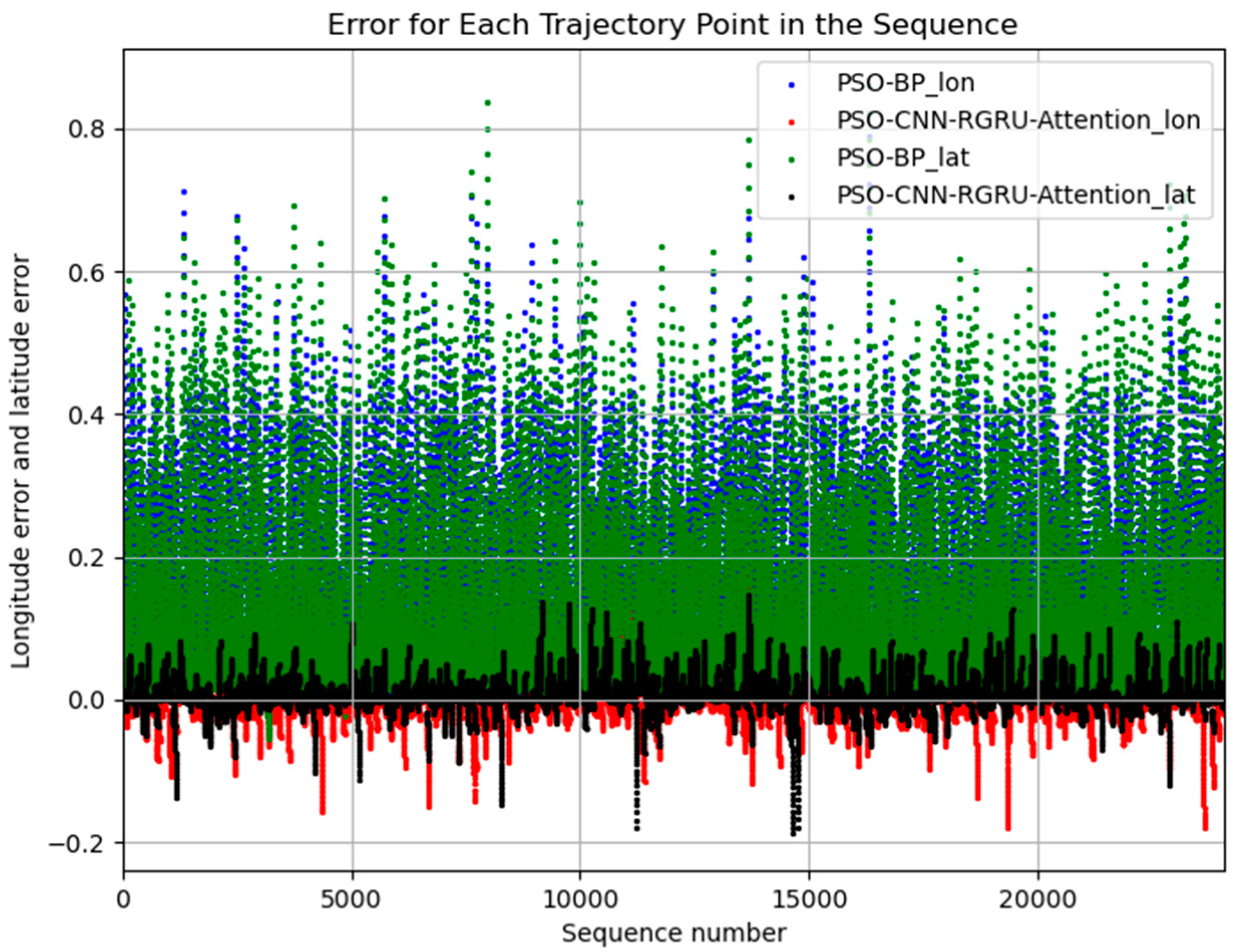
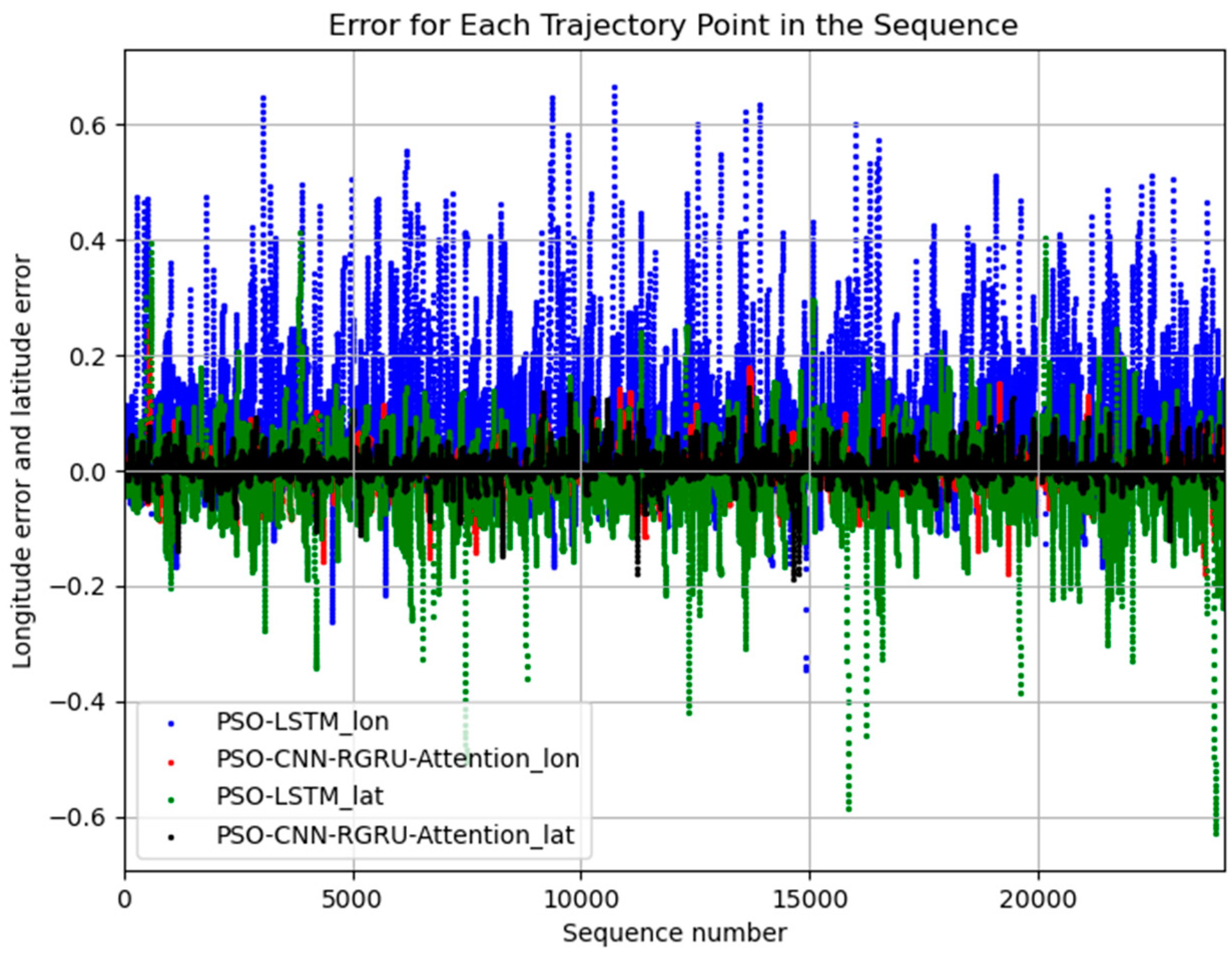
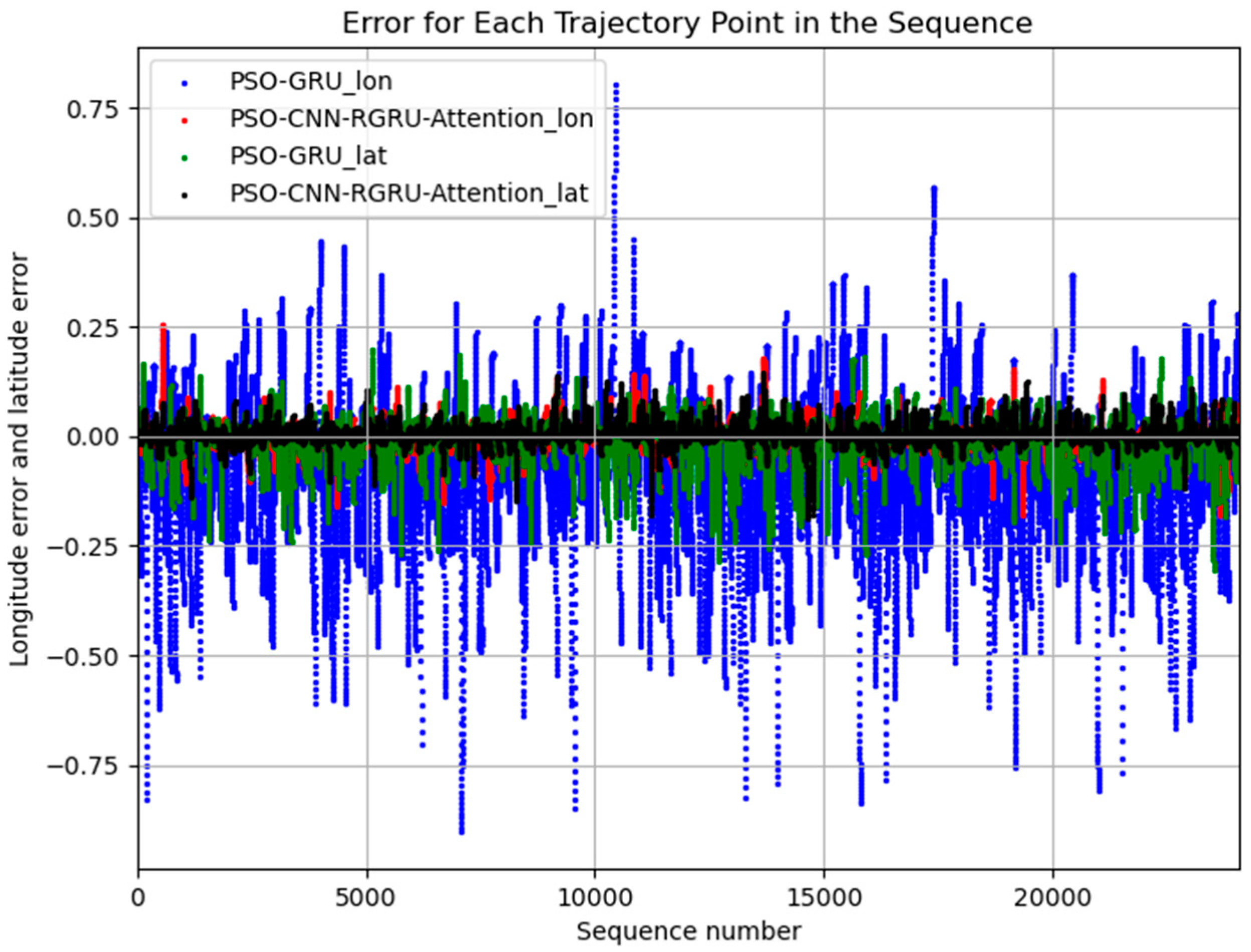
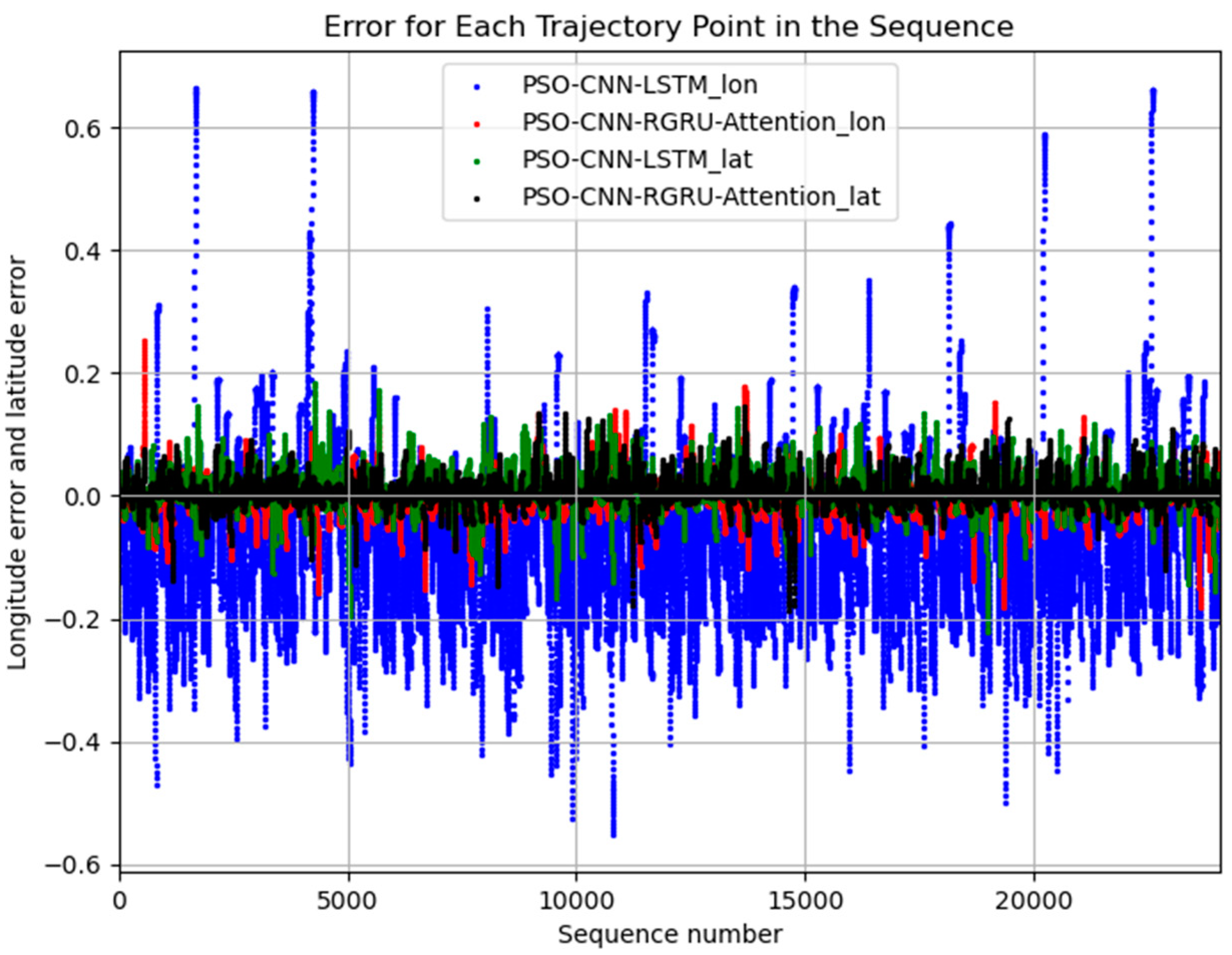
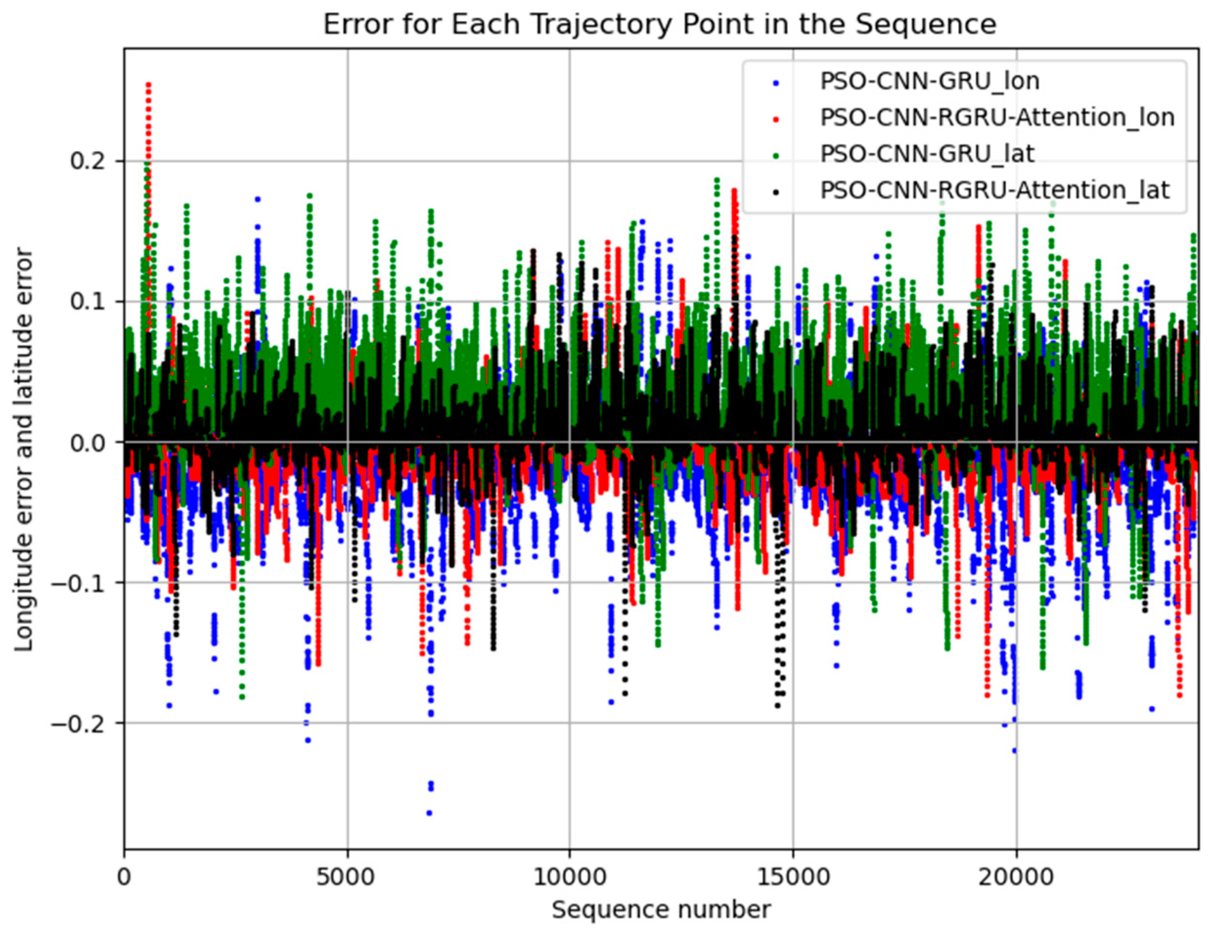
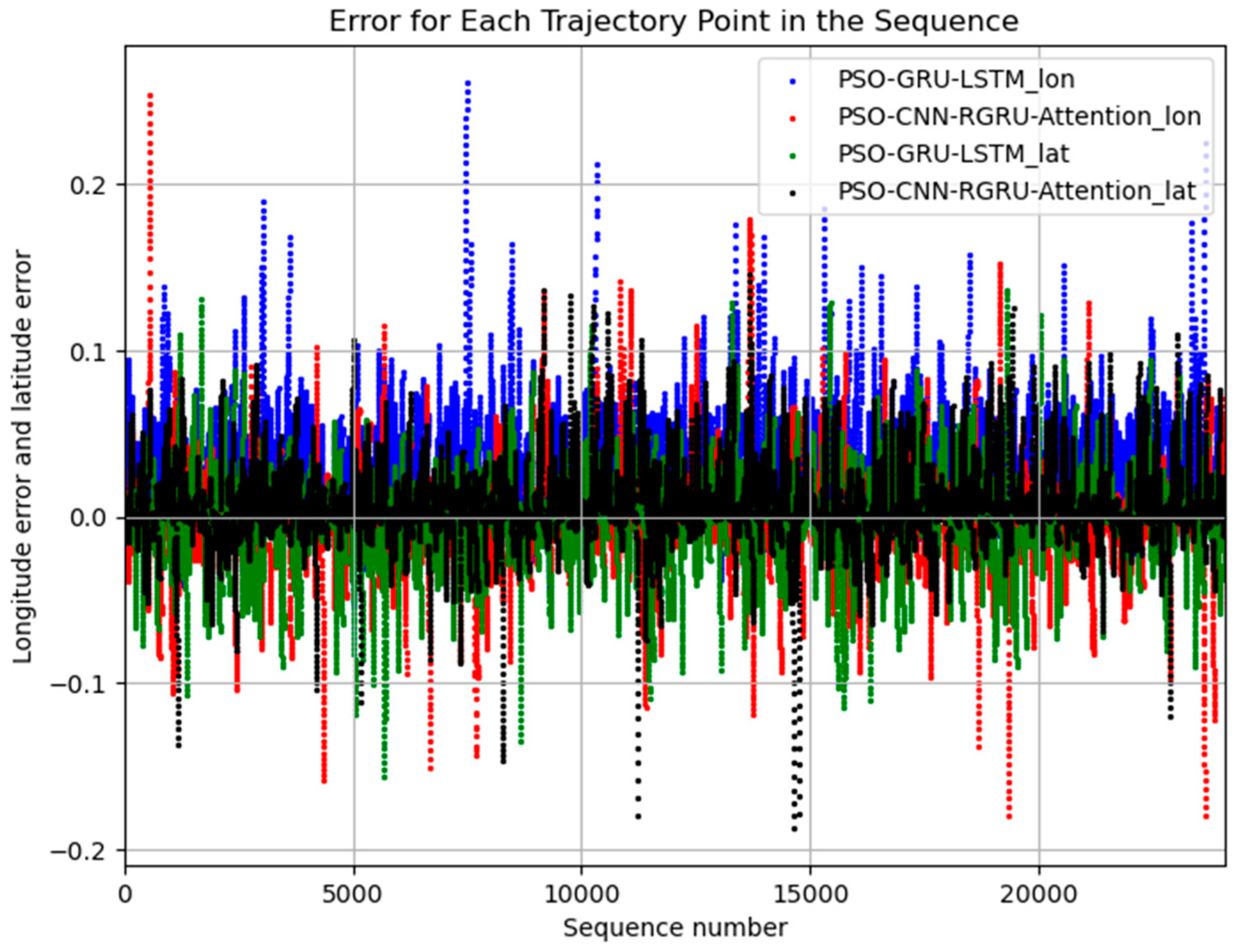
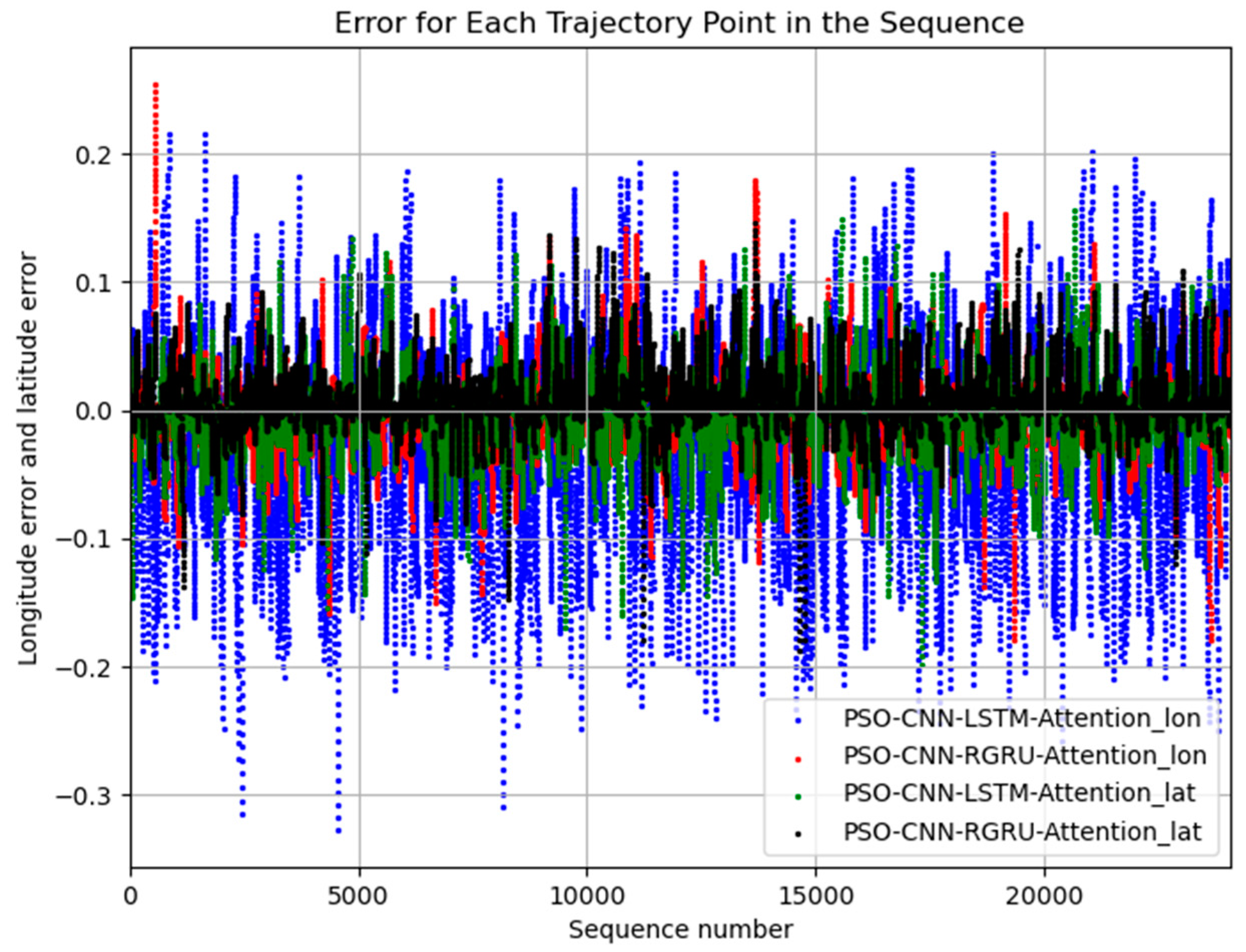
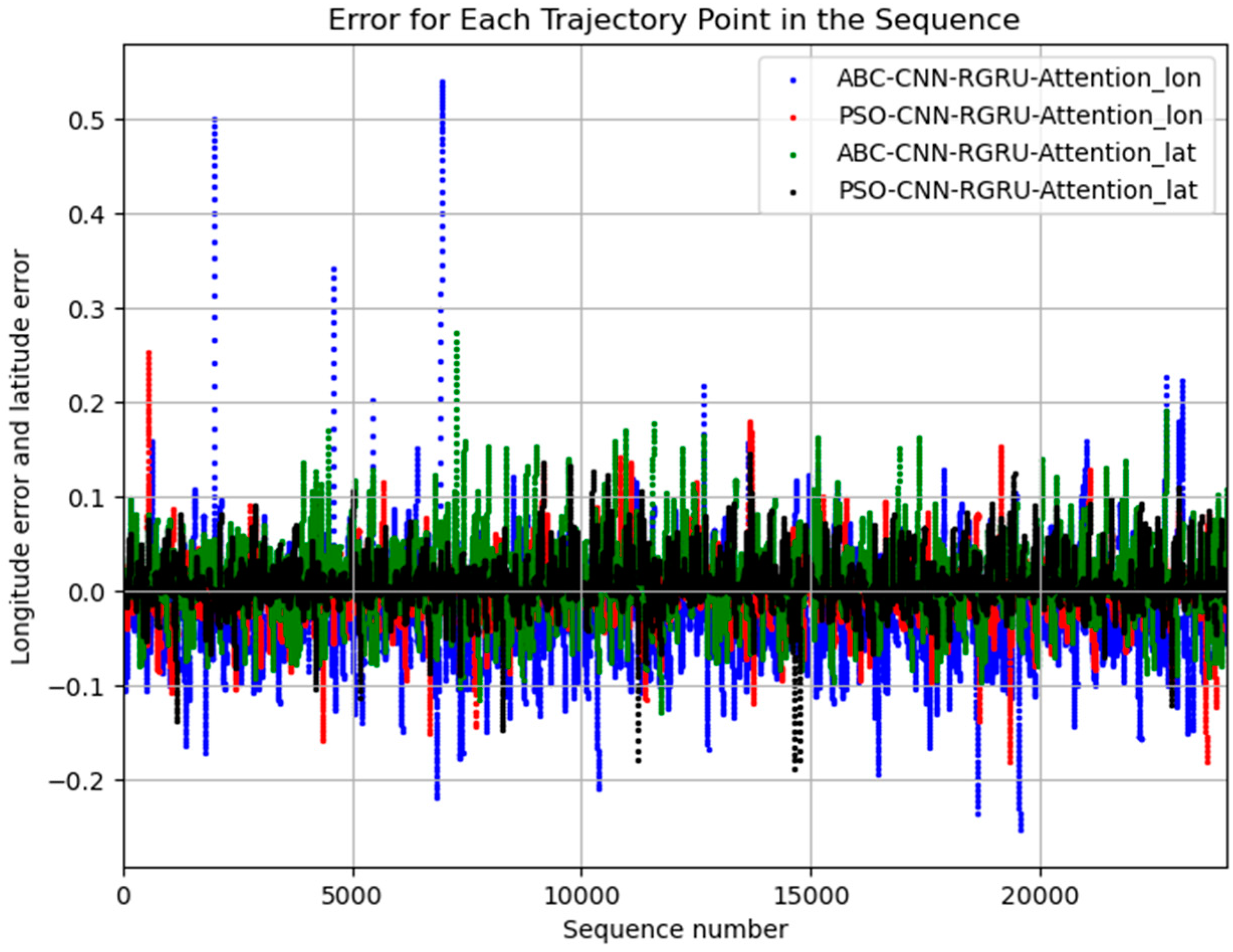
Experiment Results Analysis

In the experiment, we first performed a one-step prediction of ship trajectories, specifically predicting the trajectory at the next time step. The prediction performance of the PSO-CNN-RGRU-Attention model was compared with that of several other models: PSO-BP, PSO-LSTM, PSO-GRU, PSO-BiLSTM, PSO-BiGRU, PSO-CNN-LSTM, PSO-CNN-GRU, PSO-GRU-LSTM, PSO-CNN-LSTM-Attention, ABC-CNN-RGRU-Attention, SSA-CNN-RGRU-Attention, and WOA-CNN-RGRU-Attention. The comparison focused on prediction error and the degree of fitting.

Table 2. Comparison of Longitude Prediction Errors Among Different Models.

Model	MAE	MSE	RMSE
PSO-BP	0.05107755	0.00473161	0.06878676
PSO-LSTM	0.09581701	0.01831781	0.12556596
PSO-GRU	0.12906489	0.03170017	0.17804541
PSO-BiLSTM	0.02661157	0.00138471	0.03721178
PSO-BiGRU	0.05415891	0.00504971	0.07106135
PSO-CNN-LSTM	0.10783649	0.01916146	0.13842495
PSO-CNN-GRU	0.02387195	0.00121191	0.03481251
PSO-GRU-LSTM	0.02641866	0.00131173	0.03621787
PSO-CNN-LSTM-Attention	0.04683651	0.00427090	0.06535212
ABC-CNN-RGRU-Attention	0.03751446	0.00261446	0.05113182
SSA-CNN-RGRU-Attention	0.03133182	0.00292325	0.05406715
WOA-CNN-RGRU-Attention	0.03794286	0.00382171	0.06182004
PSO-CNN-RGRU-Attention	0.02201033	0.00117039	0.03421106

presents the comparison of longitude prediction errors for each model using the following evaluation metrics: Mean Absolute Error (MAE), Mean Squared Error (MSE), and Root Mean Squared Error (RMSE). The PSO-CNN-RGRU-Attention model demonstrated improved prediction accuracy for longitude compared to the other models, with the following reductions: MAE: reduced by 56.9%, 77.0%, 82.9%, 17.3%, 59.4%, 79.6%, 7.8%, 16.7%, 53.0%, 41.3%, 29.8%, and 42.1% relative to PSO-BP, PSO-LSTM, PSO-GRU, PSO-BiLSTM, PSO-BiGRU, PSO-CNN-LSTM, PSO-CNN-GRU, PSO-GRU-LSTM, PSO-CNN-LSTM-Attention, ABC-CNN-RGRU-Attention, SSA-CNN-RGRU-Attention, and WOA-CNN-RGRU-Attention, respectively. MSE: reduced by 75.3%, 93.4%, 96.3%, 15.5%, 76.8%, 93.8%, 3.4%, 10.8%, 72.6%, 55.2%, 60.0%, and 69.4%, respectively. RMSE: reduced by 50.3%, 72.7%, 80.9%, 8.1%, 51.9%, 75.3%, 1.7%, 5.5%, 47.6%, 33.1%, 36.7%, and 44.6%, respectively. These results indicate that the PSO-CNN-RGRU-Attention model significantly outperformed the other models in predicting ship trajectories, highlighting its effectiveness in accurately forecasting maritime movements.

Table 3. Comparison of latitude errors predicted by different models.

Model	MAE	MSE	RMSE
PSO-BP	0.03319885	0.00192588	0.04388492
PSO-LSTM	0.04516268	0.00475778	0.06897666
PSO-GRU	0.03420336	0.00276886	0.05261996
PSO-BiLSTM	0.01900496	0.00070055	0.02646798
PSO-BiGRU	0.03123733	0.00200800	0.04481072
PSO-CNN-LSTM	0.02013612	0.00087166	0.02952389
PSO-CNN-GRU	0.02916388	0.00147378	0.03838990
PSO-GRU-LSTM	0.01653731	0.00060200	0.02453578
PSO-CNN-LSTM-Attention	0.01806733	0.00075004	0.02738693
ABC-CNN-RGRU-Attention	0.02459865	0.00118986	0.03449439
SSA-CNN-RGRU-Attention	0.01623029	0.00096784	0.03111023
WOA-CNN-RGRU-Attention	0.02685349	0.00185097	0.04302294
PSO-CNN-RGRU-Attention	0.01508747	0.00054552	0.02335655

presents a comparison of the latitude prediction errors for different ship trajectory prediction models, evaluated using the metrics MAE, MSE, and RMSE. The PSO-CNN-RGRU-Attention model demonstrated superior latitude prediction accuracy compared to the PSO-BP, PSO-LSTM, PSO-GRU, PSO-BiLSTM, PSO-BiGRU, PSO-CNN-LSTM, PSO-CNN-GRU, PSO-GRU-LSTM, PSO-CNN-LSTM-Attention, ABC-CNN-RGRU-Attention, SSA-CNN-RGRU-Attention, and WOA-CNN-RGRU-Attention models. Specifically, the MAE was reduced by 54.5%, 66.6%, 55.9%, 20.6%, 51.7%, 25.1%, 48.3%, 8.8%, 16.5%, 38.7%, 7.0%, and 43.8%, respectively. The MSE decreased by 71.7%, 88.5%, 80.3%, 22.1%, 72.8%, 37.4%, 62.9%, 9.4%, 27.3%, 54.2%, 43.6%, and 70.5%, respectively. The RMSE saw reductions of 46.8%, 66.1%, 55.6%, 11.8%, 47.9%, 21.6%, 39.2%, 4.8%, 14.8%, 32.3%, 24.9%, and 45.7%, respectively.

Table 2 and Table 3 show that the PSO-CNN-RGRU-Attention model had a lower MAE, MSE, and RMSE for both longitude and latitude compared to other models. To further compare the deviation of the predicted longitude and latitude values from the actual values, we plotted the predicted trajectory sequences on the x-axis and the predicted ship’s longitude and latitude on the y-axis.

Figure 11, Figure 12, Figure 13, Figure 14, Figure 15, Figure 16, Figure 17, Figure 18, Figure 19, Figure 20, Figure 21 and Figure 22 illustrate the comparison of longitude and latitude predictions between various models and the PSO-CNN-RGRU-Attention model.

According to the visual comparison of Figure 11, Figure 12, Figure 13, Figure 14, Figure 15, Figure 16, Figure 17, Figure 18, Figure 19, Figure 20, Figure 21 and Figure 22, the PSO-CNN-RGRU-Attention model demonstrated the best fit in the longitude and latitude prediction tasks. Furthermore, by analyzing the detailed evaluation metrics in Table 2 and Table 3, it is clear that the PSO-CNN-RGRU-Attention model significantly outperformed other models, including PSO-BP, PSO-LSTM, PSO-GRU, PSO-BiLSTM, PSO-BiGRU, PSO-CNN-LSTM, PSO-CNN-GRU, PSO-GRU-LSTM, PSO-CNN-LSTM-Attention, ABC-CNN-RGRU-Attention, SSA-CNN-RGRU-Attention, and WOA-CNN-RGRU-Attention, in terms of both longitude and latitude prediction accuracy.

5. Conclusions

In this paper, various deep learning models were selected for comparison, including recurrent neural networks (BP, LSTM, GRU), bidirectional recurrent neural networks (BiLSTM, BiGRU), and hybrid neural network models (CNN-LSTM, CNN-GRU, GRU-LSTM, CNN-LSTM-Attention), as well as models combining different optimization algorithms such as ABC-CNN-RGRU-Attention, SSA-CNN-RGRU-Attention, and WOA-CNN-RGRU-Attention. By comparing the prediction errors of these models in both longitude and latitude dimensions, the PSO-CNN-RGRU-Attention model, which integrates PSO, CNN, residual networks, GRU, and attention mechanisms, demonstrated the best performance, with the lowest MAE and RMSE. The PSO-CNN-RGRU-Attention model achieved better prediction results in both longitude and latitude compared to the other models, effectively addressing navigation safety issues in this maritime area. The model’s improved performance enhances confidence in decision-making and is expected to play a significant role in fields such as traffic management and maritime safety.

Future research can further verify the performance of this model in a wider range of application scenarios by considering additional natural and human factors, thereby improving the model’s adaptability and prediction accuracy in complex environments. In addition, the use of more advanced deep learning architectures and training techniques, such as reinforcement learning or multi-task learning paradigms, should also be explored to further enhance the performance of geographic information prediction tasks.

References

1. Tu, E.; Zhang, G.; Rachmawati, L.; Rajabally, E.; Huang, G.-B. Exploiting AIS data for intelligent maritime navigation: A comprehensive survey from data to methodology. IEEE Trans. Intell. Transp. Syst. 2017, 19, 1559–1582. [Google Scholar]
2. Qiao, S.; Shen, D.; Wang, X.; Han, N.; Zhu, W. A self-adaptive parameter selection trajectory prediction approach via hidden Markov models. IEEE Trans. Intell. Transp. Syst. 2014, 16, 284–296. [Google Scholar]
3. Mazzarella, F.; Arguedas, V.F.; Vespe, M. Knowledge-based vessel position prediction using historical AIS data. In Proceedings of the 2015 Sensor Data Fusion: Trends, Solutions, Applications (SDF), Bonn, Germany, 6–8 October 2015; pp. 1–6. [Google Scholar]
4. Ma, X.; Tao, Z.; Wang, Y.; Yu, H.; Wang, Y. Long short-term memory neural network for traffic speed prediction using remote microwave sensor data. Transp. Res. Part C Emerg. Technol. 2015, 54, 187–197. [Google Scholar]
5. Zhang, Z.; Ni, G.; Xu, Y. Ship trajectory prediction based on LSTM neural network. In Proceedings of the 2020 IEEE 5th Information Technology and Mechatronics Engineering Conference (ITOEC), Chongqing, China, 12–14 June 2020; pp. 1356–1364. [Google Scholar]
6. Tang, H.; Yin, Y.; Shen, H. A model for vessel trajectory prediction based on long short-term memory neural network. J. Mar. Eng. Technol. 2022, 21, 136–145. [Google Scholar]
7. Zhang, J.; Wang, H.; Cui, F.; Liu, Y.; Liu, Z.; Dong, J. Research into ship trajectory prediction based on an improved LSTM network. J. Mar. Sci. Eng. 2023, 11, 1268. [Google Scholar] [CrossRef]
8. Han, P.; Wang, W.; Shi, Q.; Yang, J. Real-time short-term trajectory prediction based on GRU neural network. In Proceedings of the 2019 IEEE/AIAA 38th Digital Avionics Systems Conference (DASC), San Diego, CA, USA, 8–12 September 2019; pp. 1–8. [Google Scholar]
9. Yang, C.-H.; Wu, C.-H.; Shao, J.-C.; Wang, Y.-C.; Hsieh, C.-M. AIS-Based Intelligent Vessel Trajectory Prediction Using Bi-LSTM. IEEE Access 2022, 10, 24302–24315. [Google Scholar] [CrossRef]
10. Wang, C.; Ren, H.; Li, H. Vessel trajectory prediction based on AIS data and bidirectional GRU. In Proceedings of the 2020 International Conference on Computer Vision, Image and Deep Learning (CVIDL), Chongqing, China, 10–12 July 2020; pp. 260–264. [Google Scholar]
11. Cen, J.; Li, J.; Liu, X.; Chen, J.; Li, H.; Huang, W.; Zeng, L.; Kang, J.; Ke, S. A hybrid prediction model of vessel trajectory based on attention mechanism and CNN-GRU. Proc. Inst. Mech. Eng. Part M J. Eng. Marit. Environ. 2024, 238, 809–823. [Google Scholar] [CrossRef]
12. Gao, D.; Zhu, Y.; Zhang, J.; He, Y.-K.; Yan, K.; Yan, B.-R. A novel MP-LSTM method for ship trajectory prediction based on AIS data. Ocean. Eng. 2021, 228, 108956. [Google Scholar] [CrossRef]
13. Pang, S.; Zou, L.; Zhang, L.; Wang, H.; Wang, Y.; Liu, X.; Jiang, J. A hybrid TCN-BiLSTM short-term load forecasting model for ship electric propulsion systems combined with multi-step feature processing. Ocean. Eng. 2025, 316, 119808. [Google Scholar]
14. Zhao, C.D.; Zhuang, J.H.; Cheng, X.M.; Li, Y.H.; Guo, D.P. Ship trajectory prediction of RNN-Bi-LSTM based on characteristic attention mechanism. J. Guandong Ocean. Univ. 2022, 42, 102–109. [Google Scholar]
15. Gundu, V.; Simon, S.P. PSO–LSTM for short term forecast of heterogeneous time series electricity price signals. J. Ambient. Intell. Humaniz. Comput. 2021, 12, 2375–2385. [Google Scholar]
16. Li, C.; Guo, Q.; Shao, L.; Li, J.; Wu, H. Research on short-term load forecasting based on optimized gru neural network. Electronics 2022, 11, 3834. [Google Scholar] [CrossRef]
17. Mittal, S.; Sangwan, O.P. ABC LSTM optimizing parameters of deep LSTM using ABC algorithm for big datasets. Int. J. Eng. Adv. Technol. 2020, 9, 221–226. [Google Scholar] [CrossRef]
18. Luo, J.; Gong, Y. Air pollutant prediction based on ARIMA-WOA-LSTM model. Atmos. Pollut. Res. 2023, 14, 101761. [Google Scholar]
19. Liu, W.; Cao, Y.; Guan, M.; Liu, L. Research on Ship Trajectory Prediction Method Based on CNN-RGRU-Attention Fusion Model. IEEE Access 2024, 12, 63950–63957. [Google Scholar] [CrossRef]
20. Gu, J.; Wang, Z.; Kuen, J.; Ma, L.; Shahroudy, A.; Shuai, B.; Liu, T.; Wang, X.; Wang, G.; Cai, J.; et al. Recent advances in convolutional neural networks. Pattern Recognit. 2018, 77, 354–377. [Google Scholar] [CrossRef]
21. He, K.; Zhang, X.; Ren, S.; Sun, J. Deep residual learning for image recognition. In Proceedings of the IEEE Conference on Computer Vision and Pattern Recognition, Las Vegas, NV, USA, 27–30 June 2016; pp. 770–778. [Google Scholar]
22. Shen, G.; Tan, Q.; Zhang, H.; Zeng, P.; Xu, J. Deep learning with gated recurrent unit networks for financial sequence predictions. Procedia Comput. Sci. 2018, 131, 895–903. [Google Scholar]
23. Vaswani, A.; Shazeer, N.; Parmar, N.; Uszkoreit, J.; Jones, L.; Gomez, A.N.; Kaiser, Ł.; Polosukhin, I. Attention is all you need. In Proceedings of the 31st International Conference on Neural Information Processing Systems, Long Beach, CA, USA, 4–9 December 2017; Volume 30, pp. 6000–6010. [Google Scholar]
24. Koshevyy, V.; Konovets, V.; Shishkin, A. SMART digital selective calling user interface on the base of Integration maritime navigation and radiocommunication equipment. Int. J. Mar. Navig. Saf. Sea Transp. 2021, 15, 291–297. [Google Scholar]
25. Liu, Y.; Zhao, Y.; Cheng, H. Processing and Stationarity Analyzing of Accelerometer Parameter Based on Cubic Spline Interpolation. In Advances in Electronic Commerce, Web Application and Communication; Jin, D., Lin, S., Eds.; Springer: Berlin/Heidelberg, Germany, 2012; Volume 2, pp. 589–595. [Google Scholar]
Figure 1. The Convolution Principle of One-Dimensional CNN.
Applsci 15 03625 g001
Figure 2. CNN Residual Connection.
Applsci 15 03625 g002
Figure 3. Structure of the GRU Unit.
Applsci 15 03625 g003
Figure 4. Weighted Sum of the Output Values from Attention Aggregation.
Applsci 15 03625 g004
Figure 5. Model Structure of PSO-CNN-RGRU-Attention.
Applsci 15 03625 g005
Figure 6. Illustration of Trajectory Interpolation.
Applsci 15 03625 g006
Figure 7. Illustration of the Sliding Window.
Applsci 15 03625 g007
Figure 8. Optimization Algorithm Training Iteration Process.
Applsci 15 03625 g008
Figure 9. Training Graph of the PSO Algorithm Optimized Model.
Applsci 15 03625 g009
Figure 10. Comparison of Training Graphs for Optimized Algorithms.
Applsci 15 03625 g010
Figure 11. Comparison of Longitude and Latitude Errors between PSO-BP and PSO-CNN-RGRU-Attention Models.
Applsci 15 03625 g011
Figure 12. Comparison of Longitude and Latitude Errors between PSO-LSTM and PSO-CNN-RGRU-Attention Models.
Applsci 15 03625 g012
Figure 13. Comparison of Longitude and Latitude Errors between PSO-GRU and PSO-CNN-RGRU-Attention Models.
Applsci 15 03625 g013
Figure 14. Comparison of Longitude and Latitude Errors between PSO-BiLSTM and PSO-CNN-RGRU-Attention Models.
Applsci 15 03625 g014
Figure 15. Comparison of Longitude and Latitude Errors between PSO-BiGRU and PSO-CNN-RGRU-Attention Models.
Applsci 15 03625 g015
Figure 16. Comparison of Longitude and Latitude Errors between PSO-CNN-LSTM and PSO-CNN-RGRU-Attention Models.
Applsci 15 03625 g016
Figure 17. Comparison of Longitude and Latitude Errors between PSO-CNN-GRU and PSO-CNN-RGRU-Attention Models.
Applsci 15 03625 g017
Figure 18. Comparison of Longitude and Latitude Errors between PSO-GRU-LSTM and PSO-CNN-RGRU-Attention Models.
Applsci 15 03625 g018
Figure 19. Comparison of Longitude and Latitude Errors between PSO-CNN-LSTM-Attention and PSO-CNN-RGRU-Attention Models.
Applsci 15 03625 g019
Figure 20. Comparison of Longitude and Latitude Errors between ABC-CNN-RGRU-Attention and PSO-CNN-RGRU-Attention Models.
Applsci 15 03625 g020
Figure 21. Comparison of Longitude and Latitude Errors between SSA-CNN-RGRU-Attention and PSO-CNN-RGRU-Attention Models.
Applsci 15 03625 g021
Figure 22. Comparison of Longitude and Latitude Errors between WOA-CNN-RGRU-Attention and PSO-CNN-RGRU-Attention Models.
Applsci 15 03625 g022