On Anisothermal Electromagnetic Elastic Deformations in Flight in Fair Weather and Lightning Storms

Abstract

The thermomechanical effects on aircraft structures in flight are compared between fair weather and a lightning storm based on a model problem, namely, equations of anisothermal unsteady piezoelectromagnetism are solved in the particular case of a parallel-sided slab assuming (i) steady conditions and spatial dependence only on the coordinate orthogonal to the slab; (ii) the displacement vector orthogonal to the slab; (iii) the magnetic field orthogonal to the electric field, with both in the plane parallel to the sides of the slab. The exact analytical solution is obtained in the linear approximation for the displacement vector, electric and magnetic fields and temperature as function of the coordinate normal to the slab, taking into account heating by the Joule effect of Ohmic electric currents and Fourier thermal conduction. These specify the strain and stress tensors, the electric current and the heat flux. The material properties involved include the mass density, dielectric permittivity, magnetic permeability, elastic stiffness tensor, electromagnetic coupling and thermal stress tensors, pyroelectric and pyromagnetic vectors and piezoelectric and piezomagnetic tensors. The analytic results of the theory are simplified assuming (i) isotropic material properties; (ii) a steady state independent of time. The profiles as a function of the coordinate normal to the slab of the electric and magnetic fields, temperature and heat flux and displacement, strain and stress are obtained in these conditions.

1. Introduction

The fundamental equations of elasticity [1,2] are combined with electric and magnetic forces in, respectively, piezoelectricity and piezomagnetism [3], which are aspects of electromechanics [4], and the electrodynamics of continua [5] relevant to adaptive and morphing structures [6], which have many applications, including in aerospace engineering [7]. Allowing for the simultaneous presence of electric and magnetic fields in electromagnetism [8,9] leads, in combination with elasticity, to the fundamental equations of piezoelectromagnetism [10]. These equations are further extended here to include coupled thermal and electrical diffusion, that is, Fourier heat conduction [11] and Ohmic electric currents [12] and their interaction through the Onsager reciprocity relations [13]. The purpose of this work is to present the first exact analytical one-dimensional solution for a steady anisothermal thermally and electrically conducting slab in the presence of the skin effect of surface electric charges/currents, with the associated electric and magnetic forces causing elastic deformations, which are also affected by temperature gradients associated with Joule resistive heating.

The general equations of dissipative electromagnetic thermoelasticity (Section 2) are obtained in two steps: (i) using the first principle of thermodynamics to obtain the constitutive equations for anisothermal elasticity in the presence of electromagnetic fields (Section 2.1); (ii) the constitutive equations from the first principle of thermodynamics are used together with the diffusion relations from the second principle of thermodynamics in the fundamental equations of electricity, magnetism, energy and momentum (Section 2.2). The resulting fundamental equations, three vector and one scalar, specify the displacement, electric and magnetic field vectors and temperature and are simplified for isotropic media in steady conditions (Section 2.3). A one-dimensional steady solution (Section 3) of the equations of electromagnetic thermoelasticity (Section 2) is obtained for a parallel-sided slab, with dependence only on the transverse coordinate, by considering (i) the electromagnetic skin effect on the metallic structures of external electric and magnetic fields mutually orthogonal and both parallel to the slab (Figure 1), and the associated Ohmic electric currents (Section 3.1); (ii) the thermal effect of Joule dissipation of electric currents by electric resistance, specifying the temperature and heat flux (Section 3.2); (iii) the elastic displacement, strain and stress due to the combination of external pressure and electric and magnetic fields with temperature gradients (Section 3.3).

The numerical application (Section 4) of electromagnetic thermoelasticity (Section 2) to a slab in steady conditions (Section 3) considers (Tables 1 and 2) four types (Section 4.1) of materials: (i) aluminium (A), used for its lightness and good conductivity; (ii) titanium (T), used for its high strength in spite of its cost; (iii) steel (S), which is affordable and has good strength; (iv) copper (C), for its very high conductivity in spite of its weight. The simulations compare flight conditions (Table 3) at the tropopause in fair weather conditions (Table 4) and in a lightning storm (Section 4.2) and include (Section 4.3) (i) the profiles (Figures 2–9) as a function of the coordinate normal to the slab (Figure 1) of the electric and magnetic fields, temperature and heat flux and displacement, strain and stress; (ii) the values at the boundaries, that is, on the outer and inner sides of the slab (Table 5). The conclusion (Section 5) notes that, although there is a vast amount of literature on aircraft flight in adverse natural or man-made weather, like wind shears, turbulence and wakes, the combined electromagnetic and thermoelastic effects in lightning storms compared with fair weather have received less attention, and are the subject of the present paper, which may be the first which considers all effects combined.

2. Fundamental Equations of Dissipative Electromagnetic Thermoelasticity

The fundamental equations of dissipative electromagnetic thermoelasticity are the four equations of electricity, magnetism, momentum and energy/entropy (Section 2.2), with the substitution of constitutive and dissipation relations arising, respectively, from the first and second principles of thermodynamics (Section 2.1). The three vector equations and one scalar equation specify the electric and magnetic fields, the displacement vectors and the temperature, and simplify for isotropic media in a steady state (Section 2.3).

2.1. Constitutive Relations for Heat, Electricity, Magnetism and Elasticity

The first principle of thermodynamics [13] states that the change in internal energy $\mathrm{d}U$ is the sum of the work $\mathrm{d}W$ and the heat $\mathrm{d}Q$:

$$\mathrm{d}U=\mathrm{d}W+\mathrm{d}Q,$$

(1a)

The latter is specified by the product of temperature T and the change of entropy $\mathrm{d}S$:

$$\mathrm{d}Q=T\mathrm{d}S.$$

(1b)

The work for piezoelectromagnetism,

$$\mathrm{d}W=\mathrm{d}{W}_{\mathrm{u}}+\mathrm{d}{W}_{\mathrm{e}}+\mathrm{d}{W}_{\mathrm{m}},$$

(2a)

consists of three parts: (i) the elastic work [1,2] of the stress tensor ${\tau }_{ij}$ on the strain tensor $e_{ij}$:

$$\mathrm{d}{W}_{\mathrm{u}}={\tau }_{ij}\mathrm{d}{e}_{ij};$$

(2b)

(ii) the electric work [9] of the electric displacement $\mathbf{D}$ on the electric field $\mathbf{E}$:

$$\mathrm{d}{W}_{\mathrm{e}}=-\mathbf{D}·\mathrm{d}\mathbf{E};$$

(2c)

(iii) the magnetic work of the magnetic induction $\mathbf{B}$ on the magnetic field $\mathbf{H}$:

$$\mathrm{d}{W}_{\mathrm{m}}=-\mathbf{B}·\mathrm{d}\mathbf{H}.$$

(2d)

Substituting (2b), (2c) and (2d) specifies the total work (2a), and adding (1b) leads to the internal energy according to (1a):

$$\mathrm{d}U=T\mathrm{d}S-\mathbf{D}·\mathrm{d}\mathbf{E}-\mathbf{B}·\mathrm{d}\mathbf{H}+{\tau }_{ij}\mathrm{d}{e}_{ij}.$$

(3)

The internal energy (3) may be replaced as a function of state by the free energy

$$F=U-TS,$$

(4a)

whose differential is given by

$$\mathrm{d}F=-S\mathrm{d}T-\mathbf{D}·\mathrm{d}\mathbf{E}-\mathbf{B}·\mathrm{d}\mathbf{H}+{\tau }_{ij}\mathrm{d}{e}_{ij}.$$

(4b)

From (4b), it follows that the free energy has four independent variables, namely, the temperature, the electric and magnetic fields and the strain tensor,

$$F=F\left(T,\mathbf{E},\mathbf{H},e_{ij}\right),$$

(5a)

and the partial derivatives specify the dependent variables, respectively, entropy, electric displacement, magnetic induction and the stress tensor:

$$\left\{{\displaystyle \frac{\partial F}{\partial T}},{\displaystyle \frac{\partial F}{\partial \mathbf{E}}},{\displaystyle \frac{\partial F}{\partial \mathbf{H}}},{\displaystyle \frac{\partial F}{\partial e_{ij}}}\right\}=\left\{-S,-\mathbf{D},-\mathbf{B},{\tau }_{ij}\right\}.$$

(5b)

Thus, each dependent variable is a function of all independent variables, leading to the following constitutive relations:

$$\begin{array}{cc}\hfill \mathrm{d}S& ={\displaystyle \frac{c_{\mathrm{V}}}{T}}\mathrm{d}T+f_i\mathrm{d}{E}_i+h_i\mathrm{d}{H}_i+{\alpha }_{ij}\mathrm{d}{e}_{ij},\hfill \end{array}$$

(6a)

$$\begin{array}{cc}\hfill \mathrm{d}{D}_i& =f_i\mathrm{d}T+{\epsilon }_{ij}\mathrm{d}{E}_j+{\vartheta }_{ij}\mathrm{d}{H}_j+p_{ijk}\mathrm{d}{e}_{jk},\hfill \end{array}$$

(6b)

$$\begin{array}{cc}\hfill \mathrm{d}{B}_i& =h_i\mathrm{d}T+{\vartheta }_{ji}\mathrm{d}{E}_j+{\mu }_{ij}\mathrm{d}{H}_j+q_{ijk}\mathrm{d}{e}_{jk},\hfill \end{array}$$

(6c)

$$\begin{array}{cc}\hfill \mathrm{d}{\tau }_{ij}& =-{\alpha }_{ij}\mathrm{d}T-p_{kij}\mathrm{d}{E}_k-q_{kij}\mathrm{d}{H}_k+A_{ijkl}\mathrm{d}{e}_{kl},\hfill \end{array}$$

(6d)

where the coefficients are the constitutive tensors specifying the properties of matter.

Starting with the diagonal of (6a)–(6d), the constitutive tensors are (i) the specific heat at constant electric and magnetic fields and strain:

$$c_{\mathrm{V}}\equiv T{\left({\displaystyle \frac{\partial S}{\partial T}}\right)}_{\mathbf{E},\mathbf{H},e_{ij}}={\left({\displaystyle \frac{\mathrm{d}Q}{\mathrm{d}T}}\right)}_{\mathbf{E},\mathbf{H},e_{ij}}=-T{\left({\displaystyle \frac{{\partial }^{2}F}{\partial T^2}}\right)}_{\mathbf{E},\mathbf{H},e_{ij}};$$

(7)

(ii) the dielectric permittivity tensor:

$${\epsilon }_{ij}\equiv {\displaystyle \frac{\partial D_i}{\partial E_j}}=-{\displaystyle \frac{{\partial }^{2}F}{\partial E_i\partial E_j}}={\epsilon }_{ji};$$

(8a)

(iii) the magnetic permeability tensor:

$${\mu }_{ij}\equiv {\displaystyle \frac{\partial B_i}{\partial H_j}}=-{\displaystyle \frac{{\partial }^{2}F}{\partial H_i\partial H_j}}={\mu }_{ji};$$

(8b)

(iv) the elastic stiffness tensor:

$$A_{ijkl}\equiv {\displaystyle \frac{\partial {\tau }_{ij}}{\partial e_{kl}}}={\displaystyle \frac{{\partial }^{2}F}{\partial e_{ij}\partial e_{kl}}}=A_{jikl}=A_{ijlk}=A_{klij}.$$

(8c)

The six non-diagonal coupling effects have symmetries: (i) thermoelectric through the pyroelectric $f_i$ vector:

$$f_i\equiv {\displaystyle \frac{\partial S}{\partial E_i}}=-{\displaystyle \frac{{\partial }^{2}F}{\partial T\partial E_i}}={\displaystyle \frac{\partial D_i}{\partial T}};$$

(9a)

(ii) thermomagnetic through the pyromagnetic $h_i$ vector:

$$h_i\equiv {\displaystyle \frac{\partial S}{\partial H_i}}=-{\displaystyle \frac{{\partial }^{2}F}{\partial T\partial H_i}}={\displaystyle \frac{\partial B_i}{\partial T}};$$

(9b)

(iii) the electro-elastic effect through the piezoelectric $p_{ijk}$ tensor:

$$p_{ijk}={\displaystyle \frac{\partial D_i}{\partial e_{jk}}}=-{\displaystyle \frac{{\partial }^{2}F}{\partial E_i\partial e_{jk}}}=-{\displaystyle \frac{\partial {\tau }_{jk}}{\partial E_i}}=p_{ikj};$$

(10a)

(iv) the magneto-elastic effect through the piezomagnetic $q_{ijk}$ tensor:

$$q_{ijk}={\displaystyle \frac{\partial B_i}{\partial e_{jk}}}=-{\displaystyle \frac{{\partial }^{2}F}{\partial H_i\partial e_{jk}}}=-{\displaystyle \frac{\partial {\tau }_{jk}}{\partial H_i}}=q_{ikj};$$

(10b)

(v) the electromagnetic coupling tensor:

$${\vartheta }_{ij}\equiv {\displaystyle \frac{\partial D_i}{\partial H_j}}=-{\displaystyle \frac{{\partial }^{2}F}{\partial E_i\partial H_j}}={\displaystyle \frac{\partial B_j}{\partial E_i}}={\vartheta }_{ji};$$

(11a)

(vi) the thermoelastic tensor:

$${\alpha }_{ij}\equiv {\displaystyle \frac{\partial S}{\partial e_{ij}}}=-{\displaystyle \frac{{\partial }^{2}F}{\partial T\partial e_{ij}}}=-{\displaystyle \frac{\partial {\tau }_{ij}}{\partial T}}={\alpha }_{ji}.$$

(11b)

The constitutive relations (Section 2.1) are substituted in the fundamental equations of electricity, magnetism, energy and momentum (Section 2.2).

2.2. Fundamental Equations of Electricity, Magnetism, Energy and Momentum

It is assumed in the equations that follow that a dot denotes the derivative with regard to time:

$$\dot{A}\equiv {\displaystyle \frac{\partial A}{\partial t}}.$$

(12a)

The spatial derivatives with regard to the coordinates are denoted by

$${\partial }_i\equiv {\displaystyle \frac{\partial }{\partial x_i}}.$$

(12b)

In the Maxwell equation for the electric field, where $c=3.00\times {10}^8\mathrm{m}{\mathrm{s}}^{-1}$ is the speed of light in a vacuum and $e_{ijk}$ the permutation symbol, the constitutive relation is substituted for the magnetic induction (6c), leading to

$$-e_{ijk}{\partial }_j{E}_k={\dot{B}}_i=h_i\dot{T}+{\vartheta }_{ji}{\dot{E}}_j+{\mu }_{ij}{\dot{H}}_j+{\displaystyle \frac{1}{2}}{q}_{ijk}\left({\partial }_j{\dot{u}}_k+{\partial }_k{\dot{u}}_j\right),$$

(13a)

where the relation between the strain tensor $e_{ij}$ and displacement vector $u_i$ is used:

$$2e_{ij}={\partial }_i{u}_j+{\partial }_j{u}_i.$$

(13b)

The electric current density [13] is proportional to the electric field through the Ohmic electrical conductivity ${\chi }_{ij}$ and to the temperature gradient through the thermoelectric coupling tensor ${\eta }_{ij}$:

$$J_i={\chi }_{ij}{E}_j+{\eta }_{ij}{\partial }_{j}T.$$

(14a)

The Maxwell equation for the magnetic field becomes

$$c{e}_{ijk}{\partial }_j{H}_k={\dot{D}}_i+J_i=f_i\dot{T}+{\epsilon }_{ij}{\dot{E}}_j+{\vartheta }_{ij}{\dot{H}}_j+{\displaystyle \frac{1}{2}}{p}_{ijk}\left({\partial }_j{\dot{u}}_k+{\partial }_k{\dot{u}}_j\right)+{\chi }_{ij}{E}_j+{\eta }_{ij}{\partial }_{j}T,$$

(14b)

where the constitutive equation for the electric displacement (6b) and the diffusion relation for the electric field (14a) are used. The heat flux $G_i$ [13] with thermoelectric coupling corresponding to the electric current (14a) is

$$G_i=-k_{ij}{\partial }_{j}T+T{\eta }_{ij}{E}_j,$$

(15)

where $k_{ij}$ is the Fourier thermal conductivity tensor. The energy equation becomes

$$0=\rho T\dot{S}+{\partial }_i{G}_i=\rho C_{\mathrm{V}}\dot{T}+\rho T\left(f_i{\dot{E}}_i+h_i{\dot{H}}_i\right)+{\displaystyle \frac{1}{2}}\rho T{\alpha }_{ij}\left({\partial }_i{\dot{u}}_j+{\partial }_j{\dot{u}}_i\right)-k_{ij}{\partial }_i{\partial }_{j}T+{\eta }_{ij}{\partial }_i\left(T{E}_j\right),$$

(16)

using the constitutive relation for the entropy (6a) and the diffusion relation for the heat flux (15). The remaining fundamental equation is for the momentum.

The momentum equation balances the inertia force,

$$\rho {\ddot{u}}_i=E_i\left({\partial }_j{D}_j\right)+{\displaystyle \frac{1}{c}}{e}_{ijk}{J}_j{B}_k+{\partial }_j{\tau }_{ij},$$

(17)

where $\rho$ is the mass density and $\ddot{\mathbf{u}}$ the acceleration, against (i) the electric force; (ii) the magnetic force; (iii) the divergence of the stress tensor, where, in the electric force $q\mathbf{E}$, the electric charge is given by the Maxwell equation $q=𝛁·\mathbf{D}={\partial }_j{D}_j$. Substituting the constitutive relations for the electric displacement (6b), magnetic induction (6c) and stress tensor (6d) and the diffusion relation for the electric current (14a) leads to

$$\begin{array}{cc}\hfill \rho {\ddot{u}}_i& =E_i\left[f_j{\partial }_{j}T+{\epsilon }_{jl}{\partial }_j{E}_l+{\vartheta }_{jl}{\partial }_j{H}_l+{\displaystyle \frac{1}{2}}{p}_{jlk}{\partial }_j\left({\partial }_l{u}_k+{\partial }_k{u}_l\right)\right]\hfill \\ \hfill & +{\displaystyle \frac{1}{c}}{e}_{ijk}\left({\chi }_{jl}{E}_l+{\eta }_{jl}{\partial }_{l}T\right)\left[h_{k}T+{\vartheta }_{mk}{E}_m+{\mu }_{km}{H}_m+{\displaystyle \frac{1}{2}}{q}_{kmn}\left({\partial }_m{u}_n+{\partial }_n{u}_m\right)\right]\hfill \\ \hfill & -{\alpha }_{ij}{\partial }_{j}T-p_{kij}{\partial }_j{E}_k-q_{kij}{\partial }_j{H}_k+{\displaystyle \frac{1}{2}}{A}_{ijkl}{\partial }_j\left({\partial }_k{u}_l+{\partial }_l{u}_k\right).\hfill \end{array}$$

(18)

The momentum Equation (18) is in quite general form because (i) it balances the inertia force against electromagnetic forces and internal stresses, as stated in (17); (ii) it uses the linear constitutive relations (6a)–(6d), including linear thermoelastic stresses, electromagnetic coupling and piezoelectric and piezomagnetic interactions. Thus, the electric $\mathbf{E}$ and magnetic $\mathbf{H}$ fields, displacement $\mathbf{u}$ and temperature T are specified by the fundamental equations of unsteady anisothermal anisotropic piezoelectromagnetism, consisting of the equations of electricity (13a), magnetism (14b), energy (16) and momentum (18) (i) for an unsteady elastic solid subject to electromagnetic forces (17); (ii) allowing for coupled heat and electrical diffusion (14a) (15); (iii) assuming linear anisotropic medium with constant constitutive (6a)–(6d) and diffusion (14a) (15) coefficients. The fundamental equations can be applied (a) in unsteady conditions that lead to stronger electromagnetic and thermoelastic coupling; (b) to anisotropic media including both crystalline and amorphous matter. The system of equations simplifies considerably for isotropic media and steady conditions (Section 2.3).

2.3. Isotropic Media and Steady Fields

In the case of isotropic media, that is, with properties independent of direction, the constitutive (6a)–(6d) and diffusive (14a), (15) equations can depend only on scalars, the identity matrix ${\delta }_{ij}$ and the permutation symbol $e_{ijk}$, and must still satisfy symmetries like (8a)–(11b). It follows that, in an isotropic medium, the following effects cannot exist: (i/ii) the pyroelectric (9a) and pyromagnetic (9b) effects, because they are specified by vectors that are isotropic only if they vanish:

$$f_i=0=h_i;$$

(19a)

(iii/iv) the piezoelectric (10a) and piezomagnetic (10b) tensors that are of third order, which can be isotropic only if they are proportional to the third-order permutation tensor $e_{ijk}$ that is skew-symmetric in all indices (i, j, k), in contradiction with the symmetries in (10a) and (10b), respectively, so both must be zero:

$$p_{ijk}=0=q_{ijk};$$

(19b)

(v) the electromagnetic coupling tensor (11a) relates (a) the electric field and displacement, which are polar vectors, to the (b) magnetic field and induction, which are axial vectors, and thus the electromagnetic coupling is a symmetric pseudo-tensor or oriented tensor [14] that changes sign ${\vartheta }_{ij}\to -{\vartheta }_{ij}$ in a coordinate inversion relative to the origin $\mathbf{x}\to -\mathbf{x}$ and thus cannot be isotropic and must vanish:

$${\vartheta }_{ij}=0.$$

(19c)

Thus, there are no pyroelectric, pyromagnetic, piezoelectric, piezomagnetic or electromagnetic coupling effects in an isotropic medium. In contrast with (v), the (vi) dielectric permittivity (8a), (vii) magnetic permeability (8b), (viii) thermoelastic tensor (11b), (ix) Fourier thermal conductivity (15), (x) Ohmic electrical conductivity (14a) and (xi) thermoelectric coupling (14a) (15) are all symmetric absolute or non-oriented tensors relating polar vectors, and do not change sign by inversion of coordinates, so their isotropic form is the product of the identity matrix or Kronecker symbol ${\delta }_{ij}$, shown by the following scalar:

$$\left\{{\epsilon }_{ij},{\mu }_{ij},{\alpha }_{ij},k_{ij},{\chi }_{ij},{\eta }_{ij}\right\}={\delta }_{ij}\left\{\epsilon ,\mu ,\alpha ,k,\chi ,\eta \right\},$$

(20a)

where the dielectric permittivity is $\epsilon$, the magnetic permeability $\mu$, the thermal stress $\alpha$, the Fourier thermal conductivity k, the Ohmic electrical conductivity $\chi$ and the thermoelectric coupling $\eta$. Similarly, the elastic stiffness tensor (8c) in an isotropic medium must be a sum of products of identity matrices with the correct symmetries, and is thus of the following form:

$$A_{ijkl}={\nu }_1{\delta }_{ik}{\delta }_{jl}+{\nu }_2{\delta }_{ij}{\delta }_{kl},$$

(20b)

Here, the Lamé moduli of elasticity $\left({\nu }_1,{\nu }_2\right)$ may be replaced by the Young’s modulus K and Poisson ratio $\sigma$,

$${\nu }_1={\displaystyle \frac{K}{1+\sigma }},{\nu }_2={\nu }_1{\displaystyle \frac{\sigma }{1-2\sigma }},$$

(20c)

in the usual form of the stiffness tensor,

$$A_{ijkl}={\displaystyle \frac{K}{1+\sigma }}\left({\delta }_{ik}{\delta }_{jl}+{\displaystyle \frac{\sigma }{1-2\sigma }}{\delta }_{ij}{\delta }_{kl}\right),$$

(20d)

relating strain to stress.

Substitution of (19a), (19b), (19c), (20a) and (20d) in (6a)–(6d) leads to the constitutive relations for an isotropic material:

$$\begin{array}{ccc}\hfill \mathrm{d}S& ={\displaystyle \frac{c_{\mathrm{V}}}{T}}\mathrm{d}T+\alpha \mathrm{d}\left(𝛁·\mathbf{u}\right),\hfill & \end{array}$$

(21a)

$$\begin{array}{ccc}\hfill \mathrm{d}\mathbf{D}& =\epsilon \mathrm{d}\mathbf{E},\hfill & \end{array}$$

(21b)

$$\begin{array}{ccc}\hfill \mathrm{d}\mathbf{B}& =\mu \mathrm{d}\mathbf{H},\hfill & \end{array}$$

(21c)

$$\begin{array}{cc}\hfill \mathrm{d}{\tau }_{ij}& =-\alpha {\delta }_{ij}\mathrm{d}T+{\displaystyle \frac{K}{1+\sigma }}\left(\mathrm{d}{e}_{ij}+{\displaystyle \frac{\sigma }{1-2\sigma }}{\delta }_{ij}\mathrm{d}{e}_{kk}\right)\hfill \\ \hfill & =-\alpha {\delta }_{ij}\mathrm{d}T+{\displaystyle \frac{K}{2\left(1+\sigma \right)}}\left[{\partial }_i{u}_j+{\partial }_j{u}_i+{\displaystyle \frac{2\sigma }{1-2\sigma }}{\delta }_{ij}\left({\partial }_k{u}_k\right)\right]\hfill \end{array}$$

(21d)

where $\epsilon$, $\mu$, K and $\sigma$ may be taken as constant for a homogeneous medium. Similarly, the isotropic conditions (19b) apply to the thermoelectric diffusion relations (14a) and (15), leading to the electric current

$$\mathbf{J}=\chi \mathbf{E}+\eta 𝛁T,$$

(22a)

and heat flux

$$\mathbf{G}=-k𝛁T+T\eta \mathbf{E}.$$

(22b)

The fundamental equations for isotropic matter may be obtained equivalently by replacing the isotropic constitutive (21a)–(21d) and diffusion (22a)–(22b) relations in the equations of (i) electricity (13a) and (21c):

$$-𝛁\wedge \mathbf{E}=\dot{\mathbf{B}}=\mu \dot{\mathbf{H}};$$

(23)

(ii) magnetism (14b), (21b) and (22a):

$$c𝛁\wedge \mathbf{H}=\dot{\mathbf{D}}+\mathbf{J}=\epsilon \dot{\mathbf{E}}+\chi \mathbf{E}+\eta 𝛁T;$$

(24)

(iii) energy (16) and (22b):

$$0=\rho T\dot{S}+𝛁·\mathbf{G}=\rho c_{\mathrm{V}}\dot{T}+\rho T\alpha \left(𝛁·\dot{\mathbf{u}}\right)-k{𝛁}^{2}T-\eta 𝛁·\left(T\mathbf{E}\right);$$

(25)

(iv) momentum (17), (21b) and (21c):

$$\begin{array}{cc}\hfill \rho \ddot{\mathbf{u}}& =\epsilon \left(𝛁·\mathbf{E}\right)\mathbf{E}+{\displaystyle \frac{1}{c}}\left(\chi \mathbf{E}+\eta 𝛁T\right)\wedge \left(\mu \mathbf{H}\right)\hfill \\ \hfill & -\alpha 𝛁T+{\displaystyle \frac{K}{2\left(1+\sigma \right)}}\left[{\nabla }^2\mathbf{u}+{\displaystyle \frac{1}{1-2\sigma }}𝛁\left(𝛁·\mathbf{u}\right)\right],\hfill \end{array}$$

(26)

where the divergence of the stress tensor (21d) is used in vector form,

$$\begin{array}{cc}\hfill {\partial }_j{\tau }_{ij}& =-\alpha {\delta }_{ij}{\partial }_{j}T+{\displaystyle \frac{K}{2\left(1+\sigma \right)}}\left[{\partial }_j\left({\partial }_i{u}_j+{\partial }_j{u}_i\right)+{\displaystyle \frac{2\sigma }{1-2\sigma }}{\partial }_i\left({\partial }_j{u}_j\right)\right]\hfill \\ \hfill & =-\alpha {\partial }_{i}T+{\displaystyle \frac{K}{2\left(1+\sigma \right)}}{\partial }_j{\partial }_j{u}_i+{\displaystyle \frac{K}{2\left(1+\sigma \right)}}\left(1+{\displaystyle \frac{2\sigma }{1-2\sigma }}\right){\partial }_i{\partial }_j{u}_j\hfill \\ \hfill & =-\alpha 𝛁T+{\displaystyle \frac{K}{2\left(1+\sigma \right)}}\left[{\nabla }^2\mathbf{u}+{\displaystyle \frac{1}{1-2\sigma }}𝛁\left(𝛁·\mathbf{u}\right)\right].\hfill \end{array}$$

(27)

The same equations of electricity (13a)→(23), magnetism (14b)→(24), energy (16)→(25) and momentum (18)→(26) follow from anisotropic→isotropic matter using the isotropic constitutive relations—(19a), (19b), (19c), (20a) and (20d)—and diffusion relations (20a).

Thus, the electric $\mathbf{E}$ and magnetic $\mathbf{H}$ fields, displacement vector $\mathbf{u}$ and temperature T satisfy the fundamental equations of electricity (23), magnetism (24), energy (25) and momentum (26) (i) for an isotropic elastic solid subject to electromagnetic forces; (ii) with coupled heat flux and electric current; (iii) assuming constant constitutive and diffusion coefficients; (iv) in unsteady conditions. In steady conditions $\partial /\left(\partial t\right)=0$, (i) the electric field decouples (23) with zero curl:

$$𝛁\wedge \mathbf{E}=\mathbf{0};$$

(28a)

(ii) the divergence of the electric field shows it is generated by electric charges:

$$𝛁·\mathbf{E}={\displaystyle \frac{𝛁·\mathbf{D}}{\epsilon }}={\displaystyle \frac{q}{\epsilon }};$$

(28b)

(iii) the magnetic induction satisfies the following:

$$𝛁·\mathbf{B}=0;$$

(29a)

(iv) the equation of magnetism (24) also decouples considering Ohmic electric currents and no thermoelectric coupling $\eta =0$:

$$c𝛁\wedge \mathbf{H}=\chi \mathbf{E};$$

(29b)

(v) the energy equation (25) considering only thermal conduction and no thermoelectric coupling $\eta =0$ simplifies to Laplace’s equation

$${\nabla }^{2}T=0$$

(29c)

for temperature in the absence of heat sources; (vi) the momentum equation (17) with external electric charges q and currents $\mathbf{J}$ and elastic stresses (27) simplifies to

$$\alpha 𝛁T={\displaystyle \frac{K}{2\left(1+\sigma \right)}}\left[{\nabla }^2\mathbf{u}+{\displaystyle \frac{1}{1-2\sigma }}𝛁\left(𝛁·\mathbf{u}\right)\right]+q\mathbf{E}+{\displaystyle \frac{\mu }{c}}\mathbf{J}\wedge \mathbf{H}.$$

(30)

These equations are solved next in the one-dimensional case of a parallel-sided slab (Section 3).

3. Electromagnetic and Thermoelastic Effects in a Slab

The fundamental equations of electromagnetic thermoelasticity (Section 2) are solved for a parallel-sided slab in steady conditions (Section 3), specifying the variation along the thickness of (i) electromagnetic effects associated with electric and magnetic fields and electric currents (Section 3.1); (ii) thermal effects associated with temperature and heat flux (Section 3.2); (iii) elastic effects associated with displacement, strain and stress (Section 3.3).

3.1. Electromagnetic Effects: Fields and Currents

A conductor, like a metallic enclosure, acts as a “Faraday cage”, excluding external electromagnetic fields. The “Faraday cage” is more accurately a “skin effect” causing external electromagnetic fields to decay exponentially with depth or distance from the surface. The simplest representation of the electric skin effect follows from the unsteady Maxwell equation (24) omitting the magnetic field

$$\dot{\mathbf{D}}=-\mathbf{J},$$

(31)

where (i) for an isotropic medium, the electric displacement is proportional (21b) to the electric field through the dielectric permittivity:

$$\mathbf{D}=\epsilon \mathbf{E};$$

(32a)

(ii) the Ohmic electric current (22a) is proportional to the electric field through the electric conductivity in the absence of thermoelectric coupling $\eta =0$:

$$\mathbf{J}=\chi \mathbf{E}.$$

(32b)

Substitution of (32a) and (32b) in (31) gives

$$\dot{\mathbf{E}}=-{\displaystyle \frac{\chi }{\epsilon }}\mathbf{E},$$

(33)

showing that the electric field decays exponentially with time:

$$\mathbf{E}\left(t\right)={\mathbf{E}}_{0}exp\left(-{\displaystyle \frac{\chi }{\epsilon }}t\right)={\mathbf{E}}_{0}exp\left(-{\displaystyle \frac{t}{\theta }}\right),$$

(34a)

where ${\mathbf{E}}_0\equiv \mathbf{E}\left(0\right)$ is the electric field at the initial instant and with a time scale

$$\theta \equiv {\displaystyle \frac{\epsilon }{\chi }},$$

(34b)

which is small for highly conducting materials like metals. Unsteady electromagnetic fields propagate like waves at the speed of light:

$${\displaystyle \frac{x}{t}}=c_{\mathrm{em}}={\displaystyle \frac{c}{\sqrt{\epsilon \mu }}},$$

(35a)

Thus, the electric field (34a) decays exponentially with distance:

$$\mathbf{E}\left(x\right)={\mathbf{E}}_{0}exp\left(-{\displaystyle \frac{\chi }{\epsilon }}{\displaystyle \frac{x}{c_{\mathrm{em}}}}\right)={\mathbf{E}}_{0}exp\left(-\chi {\displaystyle \frac{x}{c}}\sqrt{{\displaystyle \frac{\mu }{\epsilon }}}\right)=E_{0}exp\left(-{\displaystyle \frac{x}{l}}\right){\mathbf{e}}_{\mathrm{y}};$$

(35b)

In (35b), the electric field is taken parallel to the slab in the y-direction, with surface value $E_0$, decaying exponentially with depth, with length scale or with penetration depth:

$$l\equiv c_{\mathrm{em}}\theta ={\displaystyle \frac{c}{\chi }}\sqrt{{\displaystyle \frac{\epsilon }{\mu }}}.$$

(35c)

Thus, (35c) is the length scale for the exponential decay in the depth of the “electromagnetic skin effect”, which applies not only to the electric field but also to the magnetic field and electric currents, as shown next. The Ohmic electric current (32b) has the same direction and decay as the electric field (35b),

$$\mathbf{J}\left(x\right)=J_{0}exp\left(-{\displaystyle \frac{x}{l}}\right){\mathbf{e}}_{\mathrm{y}}=\chi E_{0}exp\left(-{\displaystyle \frac{x}{l}}\right){\mathbf{e}}_{\mathrm{y}},$$

(35d)

with $J_0\equiv J\left(0\right)$ being the absolute value of the electric current at the initial instant.

The magnetic field is considered (Figure 1) parallel to the sides of the slab and orthogonal to the electric field (35b) and current (35d) as

$$\mathbf{H}\left(x\right)=H\left(x\right){\mathbf{e}}_{\mathrm{z}},$$

(36a)

to satisfy the Maxwell equation (29b) in the form

$${\displaystyle \frac{\mathbf{J}\left(x\right)}{c}}={\displaystyle \frac{J\left(x\right)}{c}}{\mathbf{e}}_{\mathrm{y}}=𝛁\wedge \left[H\left(x\right){\mathbf{e}}_{\mathrm{z}}\right]=-{\displaystyle \frac{\mathrm{d}H}{\mathrm{d}x}}{\mathbf{e}}_{\mathrm{y}},$$

(36b)

implying

$${\displaystyle \frac{\mathrm{d}H}{\mathrm{d}x}}=-{\displaystyle \frac{J\left(x\right)}{c}}=-{\displaystyle \frac{J_0}{c}}exp\left(-{\displaystyle \frac{x}{l}}\right).$$

(36c)

From (36c), it follows that the magnetic field (37a) decays exponentially, like the electric field (35b) and current (35d),

$$\mathbf{H}\left(x\right)=H_{0}exp\left(-{\displaystyle \frac{x}{l}}\right){\mathbf{e}}_{\mathrm{z}},$$

(37a)

from the surface value

$$H_0=J_0{\displaystyle \frac{l}{c}}=E_0{\displaystyle \frac{\chi l}{c}}=\sqrt{{\displaystyle \frac{\epsilon }{\mu }}}{E}_0.$$

(37b)

The relation (37b) is consistent with the equipartition

$$W_{\mathrm{e}}=W_{\mathrm{m}},$$

(38a)

of electric energy

$$W_{\mathrm{e}}={\displaystyle \frac{\mathbf{E}·\mathbf{D}}{2}}={\displaystyle \frac{\epsilon }{2}}{\left|\mathbf{E}\right|}^2,$$

(38b)

and magnetic energy

$$W_{\mathrm{m}}={\displaystyle \frac{\mathbf{B}·\mathbf{H}}{2}}={\displaystyle \frac{\mu }{2}}{\left|\mathbf{H}\right|}^2,$$

(38c)

which leads to

$$\left|\mathbf{H}\right|=\sqrt{{\displaystyle \frac{\epsilon }{\mu }}}\left|\mathbf{E}\right|.$$

(38d)

Since the electric field (35b), electric current (35d) and magnetic field (36a) all lie parallel to the sides of the slab (Figure 1), and thus orthogonal to the direction of variation, all have zero divergence:

$$\begin{array}{cc}\hfill 0& =𝛁·\mathbf{J}={\displaystyle \frac{\partial }{\partial y}}\left[J\left(x\right)\right],\hfill \end{array}$$

(39a)

$$\begin{array}{cc}\hfill 0& =𝛁·\mathbf{H}={\displaystyle \frac{\partial }{\partial z}}\left[H\left(x\right)\right],\hfill \end{array}$$

(39b)

$$\begin{array}{cc}\hfill 0& =𝛁·\mathbf{E}={\displaystyle \frac{\partial }{\partial y}}\left[E\left(x\right)\right],\hfill \end{array}$$

(39c)

$$\begin{array}{cc}\hfill q& =\epsilon 𝛁·\mathbf{E}=0,\hfill \end{array}$$

(39d)

where the first relation (39a) states the conservation of electric current in steady conditions; the second relation (39b) agrees with the Maxwell equation (29a); the third relation (39c) implies from the Maxwell equation (28b) that there is no electric charge (39d). The remaining Maxwell equation (28a) is met by

$$0=𝛁\wedge \left[E\left(x\right){\mathbf{e}}_{\mathrm{y}}\right]={\mathbf{e}}_{\mathrm{z}}{\displaystyle \frac{\mathrm{d}E}{\mathrm{d}x}}=-{\displaystyle \frac{E_0}{l}}exp\left(-{\displaystyle \frac{x}{l}}\right){\mathbf{e}}_{\mathrm{z}},$$

(40a)

but only with the approximation

$$1\gg {\displaystyle \frac{E_0}{l}}={\displaystyle \frac{E_0\chi }{c}}\sqrt{{\displaystyle \frac{\mu }{\epsilon }}}={\displaystyle \frac{\chi }{\epsilon }}{\displaystyle \frac{E_0}{c_{\mathrm{em}}}},$$

(40b)

of the large speed of electromagnetic waves, corresponding to steady conditions $c_{\mathrm{em}}\to \infty$. The electric current (35c) in the presence of electrical resistivity $1/\chi \ne 0$ specifies heating by the Joule effect, which determines the temperature and heat flux in the presence of the thermal conductivity (Section 3.2).

3.2. Thermal Effects: Temperature and Heat Flux

The Joule effect of heat production by dissipation of electric currents in a resistive medium [8,13] is specified by the heat source

$$Q=\mathbf{J}·\mathbf{E}=\chi {\left|\mathbf{E}\right|}^2={\displaystyle \frac{{\left|\mathbf{J}\right|}^2}{\chi }},$$

(41)

leading, in the case of the skin effect (35d), to the depth dependence

$$Q\left(x\right)=Q_{0}exp\left(-{\displaystyle \frac{2x}{l}}\right),$$

(42a)

with surface value

$$Q_0=E_0{J}_0=\chi {\left(E_0\right)}^2={\displaystyle \frac{{\left(J_0\right)}^2}{\chi }}.$$

(42b)

The steady heat conduction balances the heat sources Q in a domain D of volume $\mathrm{d}V$ against the heat flux $\mathbf{G}$ through the boundary $\partial D$ with area element $\mathrm{d}\mathbf{A}$:

$${\int }_{D}Q\mathrm{d}V={\int }_{\partial D}\mathbf{G}·\mathrm{d}\mathbf{A}={\int }_D\left(𝛁·\mathbf{G}\right)\mathrm{d}V,$$

(43a)

Use of the divergence theorem leads to the steady heat equation with sources [15]

$$𝛁·\mathbf{G}=Q.$$

(43b)

Using the Fourier heat flux (22b), and neglecting thermoelectric coupling,

$$\mathbf{G}=-k𝛁T$$

(44)

leads [15] to the steady heat equation with sources

$${\nabla }^{2}T=-{\displaystyle \frac{Q}{k}},$$

(45)

which specifies the temperature and reduces to (29c) in the absence of heat sources.

Thus, in the interior of the slab, the temperature satisfies

$${\displaystyle \frac{{\mathrm{d}}^{2}T}{\mathrm{d}{x}^2}}=-{\displaystyle \frac{Q\left(x\right)}{k}}=-{\displaystyle \frac{Q_0}{k}}exp\left(-{\displaystyle \frac{2x}{l}}\right)=-{\displaystyle \frac{\chi }{k}}{\left(E_0\right)}^{2}exp\left(-{\displaystyle \frac{2x}{l}}\right),$$

(46)

together with boundary conditions on the two sides. The integration of (46) specifies the temperature profile

$$T\left(x\right)=-T_{\ast }exp\left(-{\displaystyle \frac{2x}{l}}\right)+C_{1}x+C_2,$$

(47a)

where (i) the constant $T_{\ast }$ has the dimensions of temperature:

$$T_{\ast }={\displaystyle \frac{Q_0{l}^2}{4k}}={\displaystyle \frac{\chi }{4k}}{\left(E_{0}l\right)}^2={\displaystyle \frac{\epsilon }{4\mu k\chi }}{\left(E_{0}c\right)}^2;$$

(47b)

(ii) the temperature at the outer boundary specifies the constant $C_1$:

$$T_0\equiv T\left(0\right)=C_2-T_{\ast };$$

(48a)

(iii) the temperature at the inner boundary specifies the constant $C_2$:

$$T_1\equiv T\left(L\right)=-T_{\ast }exp\left(-{\displaystyle \frac{2L}{l}}\right)+C_{1}L+T_0+T_{\ast }.$$

(48b)

Solving (48a) and (48b) for $C_1$ and $C_2$, and substitution in (47a), specifies the temperature profile

$$T\left(x\right)=T_0+{\displaystyle \frac{T_1-T_0}{L}}x+T_{\ast }\left(1-{\displaystyle \frac{x}{L}}\right)-T_{\ast }\left[exp\left(-{\displaystyle \frac{2x}{l}}\right)-{\displaystyle \frac{x}{L}}exp\left(-{\displaystyle \frac{2L}{l}}\right)\right]$$

(49)

where, on the right-hand side of (49), (i) the first two terms correspond to the boundary temperatures (48a) and (48b) without sources; (ii) the last two terms are due (47b) to the Joule heating—Equations (41), (42a) and (42b). The heat flux (44) is related by

$$\mathbf{G}=-k{\displaystyle \frac{\mathrm{d}T}{\mathrm{d}x}}{\mathbf{e}}_{\mathrm{x}},$$

(50a)

to the gradient of the temperature (49):

$$\mathbf{G}\left(x\right)={\mathbf{e}}_{\mathrm{x}}k\left\{{\displaystyle \frac{T_{\ast }+T_0-T_1}{L}}-T_{\ast }\left[{\displaystyle \frac{2}{l}}exp\left(-{\displaystyle \frac{2x}{l}}\right)+{\displaystyle \frac{1}{L}}exp\left(-{\displaystyle \frac{2L}{l}}\right)\right]\right\}.$$

(50b)

The temperature gradient causes thermal stresses that, together with electromagnetic forces, balance the elastic stresses, thus specifying the displacement, strain and stress (Section 3.3).

3.3. Elastic Effects: Displacement, Strain and Stress

The magnetic force

$${\mathbf{F}}_{\mathrm{m}}={\displaystyle \frac{\mu }{c}}\mathbf{J}\wedge \mathbf{H},$$

(51a)

associated with the electric current (35d) and magnetic field (37a), is given by

$${\mathbf{F}}_{\mathrm{m}}={\displaystyle \frac{\mu }{c}}{J}_0{H}_{0}exp\left(-{\displaystyle \frac{2x}{l}}\right){\mathbf{e}}_{\mathrm{y}}\times {\mathbf{e}}_{\mathrm{z}},$$

(51b)

and thus lies in the x-direction normal to the slab and is given by

$${\mathbf{F}}_{\mathrm{m}}=\chi {\displaystyle \frac{\sqrt{\epsilon \mu }}{c}}{E}_0^{2}exp\left(-{\displaystyle \frac{2x}{l}}\right){\mathbf{e}}_{\mathrm{x}}={\displaystyle \frac{\chi }{c_{\mathrm{em}}}}{E}_0^{2}exp\left(-{\displaystyle \frac{2x}{l}}\right){\mathbf{e}}_{\mathrm{x}},$$

(51c)

where the electromagnetic wave speed (35a) appears. Taking the displacement vector in the x-direction,

$$\mathbf{u}\left(x\right)=u\left(x\right){\mathbf{e}}_{\mathrm{x}},$$

(52a)

and the only non-zero component of the strain is

$$e_{\mathrm{xx}}={\displaystyle \frac{\mathrm{d}u}{\mathrm{d}x}},$$

(52b)

and the corresponding stress (21d) is

$${\tau }_{\mathrm{xx}}\left(x\right)=-\alpha \left[T\left(x\right)-T_{\mathrm{ref}}\right]+\nu {\displaystyle \frac{\mathrm{d}u}{\mathrm{d}x}},$$

(52c)

where $T_{\mathrm{ref}}$ is a reference temperature at which the thermal stress is zero, which involves the effective elastic modulus

$$\nu ={\displaystyle \frac{K}{1+\sigma }}{\displaystyle \frac{1-\sigma }{1-2\sigma }}.$$

(53)

For steady conditions, there is no inertia force in (17), and, since there are no electric charges (39d), there is no electric force in (17), which simplifies to the balance of the magnetic force (51c) and stress (52c)

$$-F_{\mathrm{m}}={\displaystyle \frac{\mathrm{d}{\tau }_{\mathrm{xx}}}{\mathrm{d}x}},$$

(54a)

leading to the differential equation for the displacement

$$\begin{array}{cc}\hfill \nu {\displaystyle \frac{{\mathrm{d}}^{2}u}{\mathrm{d}{x}^2}}& =\alpha {\displaystyle \frac{\mathrm{d}T}{\mathrm{d}x}}-F_{\mathrm{m}}\hfill \\ \hfill & =\alpha {\displaystyle \frac{T_1-T_0-T_{\ast }}{L}}+\alpha T_{\ast }\left[{\displaystyle \frac{2}{l}}exp\left(-{\displaystyle \frac{2x}{l}}\right)+{\displaystyle \frac{1}{L}}exp\left(-{\displaystyle \frac{2L}{l}}\right)\right]-{\displaystyle \frac{\chi }{c}}\sqrt{\epsilon \mu }{E}_0^{2}exp\left(-{\displaystyle \frac{2x}{l}}\right),\hfill \end{array}$$

(54b)

which is solved next, together with boundary conditions.

The differential equation for the displacement (54b) can be rewritten as

$${\displaystyle \frac{{\mathrm{d}}^{2}u}{\mathrm{d}{x}^2}}=a+bexp\left(-{\displaystyle \frac{2x}{l}}\right),$$

(55a)

involving the constants

$$\begin{array}{cc}\hfill \nu \left\{a,b\right\}& ={\displaystyle \frac{K}{1+\sigma }}{\displaystyle \frac{1-\sigma }{1-2\sigma }}\left\{a,b\right\}\hfill \\ \hfill & =\left\{{\displaystyle \frac{\alpha }{L}}\left[T_1-T_0-T_{\ast }+T_{\ast }exp\left(-{\displaystyle \frac{2L}{l}}\right)\right],{\displaystyle \frac{2\alpha T_{\ast }}{l}}-{\displaystyle \frac{\chi }{c}}\sqrt{\epsilon \mu }{E}_0^2\right\},\hfill \end{array}$$

(55b)

where $L\gg l$, so $exp\left(-{\displaystyle \frac{2L}{l}}\right)\ll 1$, and thus the last term in square brackets can be omitted. The integration of (55a) leads to the following:

$$u\left(x\right)={\displaystyle \frac{a{x}^2}{2}}+{\displaystyle \frac{b{l}^2}{4}}exp\left(-{\displaystyle \frac{2x}{l}}\right)+C_{3}x+C_4.$$

(56)

Assuming zero displacement at the inner boundary,

$$0=u\left(L\right)={\displaystyle \frac{a{L}^2}{2}}+{\displaystyle \frac{b{l}^2}{4}}exp\left(-{\displaystyle \frac{2L}{l}}\right)+C_{3}L+C_4$$

(57a)

eliminates one constant:

$$u\left(x\right)={\displaystyle \frac{a}{2}}\left(x^2-L^2\right)+{\displaystyle \frac{b{l}^2}{4}}\left[exp\left(-{\displaystyle \frac{2x}{l}}\right)-exp\left(-{\displaystyle \frac{2L}{l}}\right)\right]+C_3\left(x-L\right).$$

(57b)

The displacement (57b) corresponds to the strain

$$e_{\mathrm{xx}}\left(x\right)=ax-{\displaystyle \frac{bl}{2}}exp\left(-{\displaystyle \frac{2x}{l}}\right)+C_3,$$

(58a)

and stress at the outer boundary balancing the atmospheric pressure

$$-p_0={\tau }_{\mathrm{xx}}\left(0\right)=\nu e_{\mathrm{xx}}\left(0\right)-\alpha \left(T_0-T_{\mathrm{ref}}\right)=\nu \left(C_3-{\displaystyle \frac{bl}{2}}\right)-\alpha \left(T_0-T_{\mathrm{ref}}\right),$$

(58b)

taking (47b) as the reference temperature for the thermal stresses. This determines the constant $C_3$,

$$C_3={\displaystyle \frac{bl}{2}}+f,$$

(58c)

involving

$$\nu f={\displaystyle \frac{K}{1+\sigma }}{\displaystyle \frac{1-\sigma }{1-2\sigma }}f=\alpha \left(T_0-T_{\mathrm{ref}}\right)-p_0,$$

(58d)

Substitution of (58d) in (57b) specifies the displacement

$$u\left(x\right)={\displaystyle \frac{a}{2}}\left(x^2-L^2\right)+{\displaystyle \frac{bl}{2}}\left(x-L\right)+f\left(x-L\right)+{\displaystyle \frac{b{l}^2}{4}}\left[exp\left(-{\displaystyle \frac{2x}{l}}\right)-exp\left(-{\displaystyle \frac{2L}{l}}\right)\right],$$

(59)

the strain

$$e_{\mathrm{xx}}\left(x\right)=f+ax+{\displaystyle \frac{bl}{2}}\left[1-exp\left(-{\displaystyle \frac{2x}{l}}\right)\right],$$

(60)

and the stress

$${\tau }_{\mathrm{xx}}\left(x\right)=\nu e_{\mathrm{xx}}\left(x\right)-\alpha \left[T\left(x\right)-T_{\mathrm{ref}}\right]=-p_0-{\displaystyle \frac{\chi l}{2c}}\sqrt{\epsilon \mu }{E}_0^2\left[1-exp\left(-{\displaystyle \frac{2x}{l}}\right)\right],$$

(61)

using (60), (58d), (55b) and (49).

The terms on the right-hand side of the stress are due to (i) the external pressure (58b); (ii) the temperature difference between the local temperature and the reference temperature; (iii) the magnetic force (51c) in a form that vanishes at the inner boundary. At the outer boundary, for a penetration depth (35c) much smaller than the thickness of the slab, the following approximation may be made:

$$l\ll L:exp\left(-{\displaystyle \frac{2L}{l}}\right)\ll 1.$$

(62a)

The reference temperature for zero thermal stresses is taken as the mean value of temperatures at the inner (48b) and outer (48a) walls:

$$T_{\mathrm{ref}}={\displaystyle \frac{T_1-T_0}{2}}.$$

(62b)

Using (62a) and (62b) in (61) leads to

$${\tau }_{\mathrm{xx}}\left(x\right)=\nu e_{\mathrm{xx}}\left(x\right)-\alpha \left[T\left(x\right)-{\displaystyle \frac{T_1-T_0}{2}}\right]=-p_0-{\displaystyle \frac{\chi l}{2c}}\sqrt{\epsilon \mu }{E}_0^2.$$

(62c)

The Joule heating by electric current (41)–(42b) affects (i) the temperature (49) and heat flux (50b) and also (ii) the displacement (59) and strain (60) through (47b), (55b) and (59) but drops out of the stress (61), where the effects (i) and (ii) cancel. The electromagnetic (Section 3.1), thermal (Section 3.2) and elastic (Section 3.3) effects (Section 3) are demonstrated next (Section 4) for four slab metals and flight at the tropopause in fair weather and a lightning storm.

4. Metal Slab in Flight in Fair and Stormy Weather

The electromagnetic, thermal and elastic variables are considered for a slab of aluminium, copper, titanium and steel (Section 4.1) in flight at the tropopause in two distinct weather conditions: fair weather with the average electric and magnetic fields of the Earth (Section 4.2); a thunderstorm with the electric and magnetic fields determined by the voltage discharge of lightning (Section 4.3).

4.1. Application to Aluminium, Copper, Titanium and Steel Plates

The deformation of a slab by temperature gradients in the presence of electric charges and currents is of interest for mechanical structures such as (i) electrostatic speakers that use electric currents to cause unsteady deformations of a membrane radiating sound; (ii) magnetostatic loudspeakers that use electric currents for the same purpose; (iii) plates of aluminium 2024 and related alloys that are extensively used in aeronautics; (iv) copper that has a higher thermal conductivity than aluminium but lower strength; (v) titanium that has a higher strength than aluminium and steel but a higher cost; (vi) steel which combines strength with low cost; (vii) PZT, which is a piezoelectric material widely used in adaptive and morphing structures and is anisotropic. Within the assumptions of the present theory, the relevant physical properties [16,17] are indicated in

Table 1. Basic physical properties of four distinct metals [16,17].

Case		A	C	S	T	Unit
Quantity	Symbol	Aluminium	Copper	Steel	Titanium
Young’s modulus	K	$7.0\times {10}^{10}$	$1.3\times {10}^{11}$	$2.0\times {10}^{11}$	$1.2\times {10}^{11}$	$\mathrm{kg}{\mathrm{m}}^{-1}{\mathrm{s}}^{-2}$
Poisson ratio	$\sigma$	$3.3\times {10}^{-1}$	$3.4\times {10}^{-1}$	$2.9\times {10}^{-1}$	$3.2\times {10}^{-1}$	−
Linear expansion coefficient	$\beta$	$2.3\times {10}^{-5}$	$1.7\times {10}^{-5}$	$1.1\times {10}^{-5}$	$8.6\times {10}^{-6}$	${\mathrm{K}}^{-1}$
Thermal conductivity	k	$2.4\times {10}^2$	$4.0\times {10}^2$	$5.2\times {10}^1$	$2.2\times {10}^2$	$\mathrm{kg}\mathrm{m}{\mathrm{s}}^{-3}{\mathrm{K}}^{-1}$
Ohmic electrical conductivity	$\chi$	$3.8\times {10}^7$	$6.0\times {10}^7$	$7.0\times {10}^6$	$2.4\times {10}^6$	${\mathrm{kg}}^{-1}{\mathrm{m}}^{-3}{\mathrm{s}}^3{\mathrm{A}}^2$
Magnetic permeability	$\mu$	$1.3\times {10}^{-6}$	$1.3\times {10}^{-6}$	$1.3\times {10}^{-4}$	$1.3\times {10}^{-6}$	$\mathrm{kg}\mathrm{m}{\mathrm{s}}^{-2}{\mathrm{A}}^{-2}$
Dielectric permittivity	$\epsilon$	$8.5\times {10}^{-12}$ *	$8.5\times {10}^{-12}$ **	$8.5\times {10}^{-14}$ ***	$8.5\times {10}^{-12}$ ****	${\mathrm{kg}}^{-1}{\mathrm{m}}^{-3}{\mathrm{s}}^4{\mathrm{A}}^2$
Mass density	$\rho$	$2.7\times {10}^3$	$9.0\times {10}^3$	$7.9\times {10}^3$	$4.5\times {10}^3$	$\mathrm{kg}{\mathrm{m}}^{-3}$

* aluminium powder, Al. ** cupric oxide, CuO. *** carbon dioxide, CO₂. **** titanium dioxide, TiO₂.

for the cases of (A) aluminium, (C) copper, (S) carbon steel and (T) titanium. The numerical examples that follow use the SI thermomechanical and electromagnetic units indicated in Appendix A.

The physical properties [16,17] indicated in Table 1 are (i/ii) the Young’s modulus E and Poisson ratio $\sigma$, which are the elastic moduli in Hooke’s law (21d); (iii) the thermal conductivity k in the heat flux (22b); (iv) the Ohmic electrical conductivity $\chi$ in the electric current (22a); (v) the dielectric permittivity $\epsilon$ relating (21b) electric displacement $\mathbf{D}$ to electric field $\mathbf{E}$; (vi) the magnetic permeability $\mu$ relating (21c) the magnetic induction $\mathbf{B}$ to the magnetic field $\mathbf{H}$; (vii) the mass density $\rho$ for reference purposes, since it appears only in the inertia force in the unsteady momentum equation (17) but drops out in the steady case; (viii) the coefficient of thermal expansion

$$\beta \equiv {\displaystyle \frac{1}{3V}}\left({\displaystyle \frac{\partial V}{\partial T}}\right),$$

(63a)

where V is the volume that is distinct from the coefficient of thermal stress

$$\alpha \equiv -{\displaystyle \frac{\partial {\tau }_{\mathrm{xx}}}{\partial T}},$$

(63b)

which appears in (21d) the direct Hooke law

$${\tau }_{ij}=-\alpha \left(T-T_{\mathrm{ref}}\right){\delta }_{ij}+{\displaystyle \frac{K}{1+\sigma }}\left(e_{ij}+{\displaystyle \frac{\sigma }{1-2\sigma }}{e}_{kk}{\delta }_{ij}\right),$$

(63c)

whose relation is obtained subsequently for inclusion in the table of derived quantities (

Table 2. Physical properties derived from Table 1.

Case			A	C	S	T	Unit
Quantity	Symbol	Equation	Aluminium	Copper	Steel	Titanium
Coefficient of thermal stress	$\alpha$	(67)	$4.7\times {10}^6$	$6.9\times {10}^6$	$5.2\times {10}^6$	$2.9\times {10}^6$	$\mathrm{kg}{\mathrm{m}}^{-1}{\mathrm{s}}^{-2}{\mathrm{K}}^{-1}$
Decay time	$\theta$	(34b)	$2.2\times {10}^{-19}$	$1.4\times {10}^{-19}$	$1.2\times {10}^{-20}$	$3.6\times {10}^{-18}$	$\mathrm{s}$
Penetration depth	l	(35c)	$6.7\times {10}^{-11}$	$4.2\times {10}^{-11}$	$3.6\times {10}^{-12}$	$1.1\times {10}^{-9}$	$\mathrm{m}$
Effective elastic modulus	$\nu$	(53)	$7.0\times {10}^{10}$	$1.3\times {10}^{11}$	$2.0\times {10}^{11}$	$1.2\times {10}^{11}$	$\mathrm{kg}{\mathrm{m}}^{-1}{\mathrm{s}}^{-2}$

); (ix) the cross-coupling coefficient $\eta$ between the heat flux (22b) and electric current (22a), which is assumed to be negligible, and is omitted from Table 1. Due to the lack of reliable values for the dielectric permittivity of metals, an estimated value in the SI system $c=1$ is obtained assuming that the electromagnetic wave speed (35a) equals that in a vacuum

$$c_{\mathrm{em}}=3.00\times {10}^8\mathrm{m}{\mathrm{s}}^{-1},$$

(64a)

so that the dielectric permittivity is calculated from the magnetic permeability

$$\epsilon ={\displaystyle \frac{1}{\mu {\left(c_{\mathrm{em}}\right)}^2}}={\displaystyle \frac{1.11\times {10}^{-17}{\mathrm{m}}^{-1}\mathrm{s}}{\mu }}.$$

(64b)

The relation between the coefficient of thermal expression (63a) and the coefficient of thermal stress (63b) is obtained in four steps: (i) the direct Hooke law (21d), equivalent to (63c), is used to relate the trace ${\tau }_{ii}$ of the stress tensor, equal to $-3p$, where p is the pressure, to the trace of the strain tensor $e_{ii}$, equal to the dilatation $𝛁·\mathbf{u}$:

$$-3p={\tau }_{ii}=-\alpha \left(T-T_{\mathrm{ref}}\right){\delta }_{ii}+{\displaystyle \frac{K}{1+\sigma }}{e}_{kk}\left(1+{\displaystyle \frac{\sigma }{1-2\sigma }}{\delta }_{ii}\right)=-3\alpha \left(T-T_{\mathrm{ref}}\right)+{\displaystyle \frac{K}{1-2\sigma }}{e}_{kk};$$

(65)

(ii) substitution of (65) in the last term of the direct stress–strain Hooke law (63c), leading to the inverse strain–stress Hooke law:

$$e_{ij}={\displaystyle \frac{1-2\sigma }{K}}\alpha \left(T-T_{\mathrm{ref}}\right){\delta }_{ij}+{\displaystyle \frac{1+\sigma }{K}}{\tau }_{ij}-{\displaystyle \frac{\sigma }{K}}{\tau }_{kk}{\delta }_{ij};$$

(66a)

(iii) the inverse Hooke law, which must be of the following form:

$$e_{ij}=\beta \left(T-T_{\mathrm{ref}}\right){\delta }_{ij}+{\displaystyle \frac{1+\sigma }{K}}{\tau }_{ij}-{\displaystyle \frac{\sigma }{K}}{\tau }_{kk}{\delta }_{ij},$$

(66b)

where the thermal expansion coefficient (63a) appears; (iv) comparing (66a)≡(66b), which leads to the relation

$$\alpha ={\displaystyle \frac{K}{1-2\sigma }}\beta ,$$

(67)

expressing the thermal stress coefficient (63b) in terms of the coefficient of thermal expansion (63a).

Table 2 indicates the physical properties derived from those in Table 1, namely, (i) the thermal stress coefficient (67); (ii) the decay time (34b); (iii) the decay length scale or penetration depth (35c); (iv) the effective elastic modulus (53).

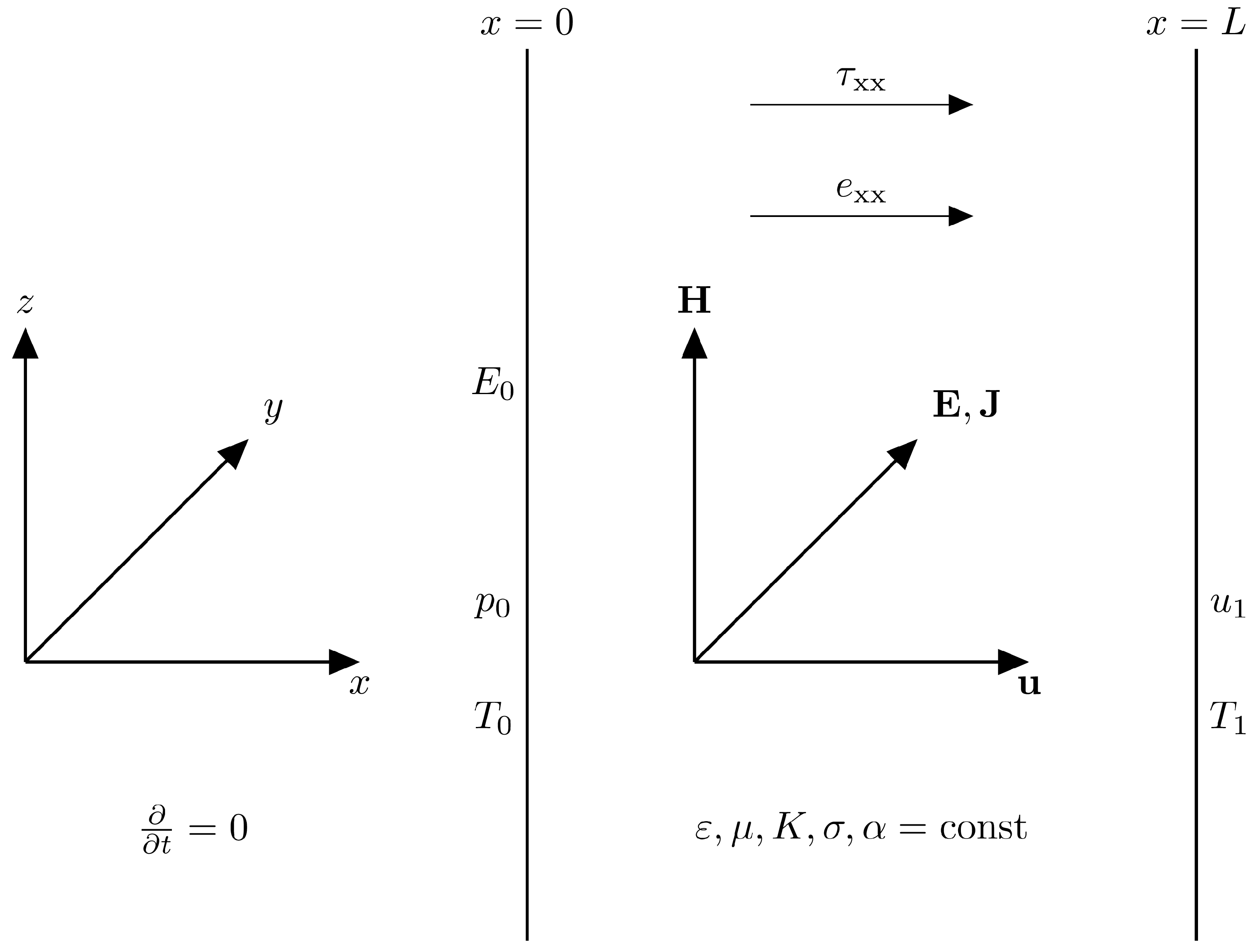
The basic and derived physical parameters in Table 1 and Table 2, respectively, appear in the profiles as a function of the depth of the eight physical variables, namely, (i–iii) the electric field (35b), current (35d) and the magnetic field (37a)–(37b)

$$\left\{\mathbf{E}\left(x\right),\mathbf{J}\left(\mathbf{x}\right),\mathbf{H}\left(\mathbf{x}\right)\right\}=exp\left(-{\displaystyle \frac{x}{l}}\right)\left\{E_0{\mathbf{e}}_{\mathrm{y}},\chi E_0{\mathbf{e}}_{\mathrm{y}},\sqrt{{\displaystyle \frac{\epsilon }{\mu }}}{E}_0{\mathbf{e}}_{\mathrm{z}}\right\},$$

(68)

for an external electric field $E_0$; (iv) the temperature profile (49) with temperature at the outer (48a) and at the inner (48b) boundaries; (v) heat flux (50b), which takes the values at the outer and at the inner boundaries:

$$\begin{array}{c}\hfill \mathbf{G}\left(0\right)={\mathbf{e}}_{\mathrm{x}}k\left\{{\displaystyle \frac{T_{\ast }+T_0-T_1}{L}}-T_{\ast }\left[{\displaystyle \frac{1}{L}}exp\left(-{\displaystyle \frac{2L}{l}}\right)+{\displaystyle \frac{2}{l}}\right]\right\},\end{array}$$

(69a)

$$\begin{array}{c}\hfill \mathbf{G}\left(L\right)={\mathbf{e}}_{\mathrm{x}}k\left\{{\displaystyle \frac{T_{\ast }+T_0-T_1}{L}}-T_{\ast }\left({\displaystyle \frac{1}{L}}+{\displaystyle \frac{2}{l}}\right)exp\left(-{\displaystyle \frac{2L}{l}}\right)\right\};\end{array}$$

(69b)

(vi) displacement (59), which vanishes at the inner boundary (57a) and takes the value

$$u_0\equiv u\left(0\right)=-{\displaystyle \frac{L}{2}}\left(aL+bl\right)+{\displaystyle \frac{b{l}^2}{4}}\left[1-exp\left(-{\displaystyle \frac{2L}{l}}\right)\right]-fL,$$

(70)

at the outer boundary; (vii) strain (60), which takes the value

$$e_{\mathrm{xx}}\left(0\right)=f={\displaystyle \frac{1}{\nu }}\left[-p_0+\alpha \left(T_0-T_{\mathrm{ref}}\right)\right]$$

(71a)

at the outer and

$$e_{\mathrm{xx}}\left(L\right)=f+aL+{\displaystyle \frac{bl}{2}}\left[1-exp\left(-{\displaystyle \frac{2L}{l}}\right)\right]$$

(71b)

at the inner boundaries; (viii) stress (61), which equals minus the atmospheric pressure at the outer boundary (58b) and takes the value

$${\tau }_{\mathrm{xx}}\left(L\right)=-p_0-{\displaystyle \frac{\chi l}{2c}}\sqrt{\epsilon \mu }{E}_0^2\left[1-exp\left(-{\displaystyle \frac{2L}{l}}\right)\right]$$

(72)

at the inner boundary.

The approximation (62a) allows the omissions of (i) the first term in square brackets in (69a); (ii) the first term in curved brackets in (69b); (iii–v) the last terms in square brackets in (70), (71b) and (72). The only remaining data needed concern the boundary values for (a) the electric field at the outer boundary:

$$E_0\equiv E\left(0\right);$$

(73)

(b,c) temperature at the outer and inner boundaries:

$$\begin{array}{cc}\hfill T_0& \equiv T\left(0\right),\hfill \end{array}$$

(74a)

$$\begin{array}{cc}\hfill T_1& \equiv T\left(L\right);\hfill \end{array}$$

(74b)

(d) pressure or stress at the outer boundary:

$${\tau }_{\mathrm{xx}}\left(0\right)=-p_0.$$

(75)

These boundary values are indicated in

Table 3. Parameters for flight at the tropopause.

Quantity	Symbol	Equation	Value	Unit
Thickness of slab	L	(76)	$2.00\times {10}^{-3}$	$\mathrm{m}$
External pressure	$p_0$	(77)	$2.27\times {10}^4$	$\mathrm{kg}{\mathrm{m}}^{-1}{\mathrm{s}}^{-2}$
External temperature	$T_0$	(78)	$216.5$	$\mathrm{K}$
Internal temperature	$T_1$	(79)	293	$\mathrm{K}$
External electric field
— Fair weather	$E_0$	(80)	$1\times {10}^2$	$\mathrm{kg}{\mathrm{m}}^2{\mathrm{s}}^{-3}{\mathrm{A}}^{-1}$
— Lightning storm	${\overline{E}}_0$	(82)	$1.95\times {10}^8$	$\mathrm{kg}{\mathrm{m}}^2{\mathrm{s}}^{-3}{\mathrm{A}}^{-1}$

for flight at the tropopause in two cases (Section 4.2): (a) in fair weather with the average electric field of the Earth; (b) in a lightning storm with the electric field specified by the voltage of the discharge.

4.2. Flight at the Tropopause in Fair Weather

The aluminium 2024 plate used in many applications, including aeronautics, is often supplied with a thickness of $L=4.26\mathrm{mm}$. The plate thickness used in aeronautics is usually 1 or $2\mathrm{mm}$ for fuselage panels and 2 or $3\mathrm{mm}$ for wing skins. A panel thickness

$$L=2\mathrm{mm}=2\times {10}^{-3}\mathrm{m},$$

(76)

is chosen. The same value is used for all four metals for comparison purposes. The coordinate x varies between (i) the outer surface in contact with the atmosphere $x=0$ and (ii) the inner surface $x=L$ corresponding to the wall of the passenger or cargo cabin. For flight at the tropopause at the altitude $z=11\mathrm{km}$, in [18,19], the International Standard Atmosphere (ISA) the pressure is

$$p_0=2.27\times {10}^4\mathrm{Pa}=2.27\times {10}^4\mathrm{kg}{\mathrm{m}}^{-1}{\mathrm{s}}^{-2},$$

(77)

and the temperature is

$$T_0=-56.5 °\mathrm{C}=216.5\mathrm{K}.$$

(78)

The internal temperature is taken as the following comfortable value in an air-conditioned cabin:

$$T_1=20 °\mathrm{C}=293\mathrm{K}.$$

(79)

For flight in fair weather, the surface electric field is taken [20] as the average value on the surface of the Earth:

$$E_0=100\mathrm{V}{\mathrm{m}}^{-1}={10}^2\mathrm{kg}\mathrm{m}{\mathrm{s}}^{-3}{\mathrm{A}}^{-1}.$$

(80)

The physical conditions during lightning storms [20,21] can be quite different from the average Earth conditions in fair weather. For example, the electric and magnetic fields in fair weather are the average Earth values, whereas, for a lightning storm, they should be calculated from the electric discharge. Lightning storms are associated with cumulonimbus clouds, which can extend over a wide altitude range from 0.5 to 16 km. Most lightning strikes on aircraft occur in low-level flight between the clouds and the ground. Lightning strikes on aircraft can also occur at high altitude near cumulonimbus clouds, although these are usually associated with storms, and are thus best avoided. Lightning strikes can occur up to 15 km from the clouds. The lightning strikes associated with thunderstorms can vary considerably from one event to another, and some indicative values are (a) a lightning strike can reach ${10}^8$–${10}^9\mathrm{V}$, that is up to $1\mathrm{GV}$, with an average value of ${\Phi }_{\mathrm{p}}=300\mathrm{MV}=3\times {10}^8\mathrm{V}$; (b) the duration of a lightning flash is $t_{\mathrm{f}}=6.5\times {10}^{-5}\mathrm{s}$; (c) a lightning storm can consist of about $N_{\mathrm{f}}=10$ flashes in close succession, lasting about $\overline{t}=0.5\mathrm{s}$. Since the present theory is steady, an average voltage $\tilde{\Phi }={\Phi }_{\mathrm{m}}{t}_{\mathrm{f}}{N}_{\mathrm{f}}/\overline{t}=3.9\times {10}^5\mathrm{V}$ is considered,

$$\overline{\Phi }=3.9\times {10}^5\mathrm{V}=3.9\times {10}^5\mathrm{kg}{\mathrm{m}}^2{\mathrm{s}}^{-3}{\mathrm{A}}^{-1},$$

(81)

using an overbar to distinguish quantities in a lightning storm from fair weather; (ii) the external electric field is calculated from the average voltage and the thickness of the slab:

$${\overline{E}}_0={\displaystyle \frac{\overline{\Phi }}{L}}=1.95\times {10}^8\mathrm{V}{\mathrm{m}}^{-1}=1.95\times {10}^8\mathrm{kg}{\mathrm{m}}^2{\mathrm{s}}^{-3}{\mathrm{A}}^{-1};$$

(82)

The value taken for the surface electric field in a lightning storm (82) is much higher than (80) for fair weather [21].

The boundary and atmospheric values in Table 3, together with the basic and derived physical properties in Table 1 and Table 2, respectively, specify in

Table 4. Parameters for flight in fair weather (lightning storm).

Quantity	Symbol	Equation	Value				Unit
			A	C	S	T
Surface electric current	$J_0$	(83)	$3.8\times {10}^9$	$6.0\times {10}^9$	$7.0\times {10}^8$	$2.4\times {10}^8$	m−2A
	$\left({\overline{J}}_0\right)$		$\left(7.4\times {10}^{15}\right)$	$\left(1.2\times {10}^{16}\right)$	$\left(1.4\times {10}^{15}\right)$	$\left(4.7\times {10}^{14}\right)$
Surface magnetic field	$H_0$	(84a)	$2.6\times {10}^{-1}$	$2.6\times {10}^{-1}$	$2.6\times {10}^{-3}$	$2.6\times {10}^{-3}$	m−1A
	$\left({\overline{H}}_0\right)$		$\left(5.0\times {10}^5\right)$	$\left(5.0\times {10}^5\right)$	$\left(5.0\times {10}^3\right)$	$\left(5.0\times {10}^5\right)$
Heating function at surface	$Q_0$	(42b)	$3.8\times {10}^{11}$	$6.0\times {10}^{11}$	$7.0\times {10}^{10}$	$2.4\times {10}^{10}$	kg m−1s−1
	$\left({\overline{Q}}_0\right)$		$\left(1.4\times {10}^{24}\right)$	$\left(2.3\times {10}^{24}\right)$	$\left(2.7\times {10}^{23}\right)$	$\left(9.1\times {10}^{22}\right)$
Reference temperature	$T_{\ast }$	(47b)	$1.8\times {10}^{-12}$	$6.8\times {10}^{-13}$	$4.5\times {10}^{-15}$	$3.1\times {10}^{-11}$	K
	$\left({\overline{T}}_{\ast }\right)$		$\left(6.8\right)$	$\left(2.6\right)$	$\left(1.7\times {10}^{-2}\right)$	$\left(1.2\times {10}^2\right)$
First parameter	a	(55b)	$1.7$	$1.3$	$7.6\times {10}^{-1}$	$6.4\times {10}^{-1}$	m−1
	$\left(\overline{a}\right)$		$\left(1.6\right)$	$\left(1.3\right)$	$\left(7.6\times {10}^{-1}\right)$	$\left(-3.4\times {10}^{-1}\right)$
Second parameter	b	(55b)	$2.4\times {10}^{-6}$	$1.1\times {10}^{-6}$	$4.8\times {10}^{-8}$	$9.7\times {10}^{-7}$	m−1
	$\left(\overline{b}\right)$		$\left(9.2\times {10}^6\right)$	$\left(4.1\times {10}^6\right)$	$\left(1.8\times {10}^5\right)$	$\left(3.7\times {10}^6\right)$
Third parameter	f	(58d)	$-1.7\times {10}^{-3}$	$-1.3\times {10}^{-3}$	$-7.6\times {10}^{-4}$	$-6.4\times {10}^{-4}$	kg m−1s−2
	$\left(\overline{f}\right)$		$\left(-1.7\times {10}^{-3}\right)$	$\left(-1.3\times {10}^{-3}\right)$	$\left(-7.6\times {10}^{-4}\right)$	$\left(-6.4\times {10}^{-4}\right)$

several parameters that (a) depend on the material, namely, aluminium (A), copper (C), steel (S) and titanium (T); (b) are different in fair weather (no overbar) and in a lightning storm (with overbar). The seven parameters listed in Table 4 are (i) from (32b) the surface electric current:

$$J_0=\chi E_0;$$

(83)

(ii) from (37b) the surface magnetic field:

$$H_0=\sqrt{{\displaystyle \frac{\epsilon }{\mu }}}{E}_0,$$

(84a)

which can be simplified using (64b),

$$H_0={\displaystyle \frac{E_0}{c_{\mathrm{em}}\mu }};$$

(84b)

(iii) the surface value of the Joule heating (42b); (iv) the temperature (47b); (v) the first parameter in (55b), which, on account of (62a) and the smallness of $T_{\ast }\ll T_1-T_0$, simplifies to

$$a={\displaystyle \frac{\alpha }{\nu }}{\displaystyle \frac{T_1-T_0}{L}};$$

(85)

(vi) the second parameter in (55b), which, on account of (47b) and (35a), can be rewritten as

$$b=\chi E_0^2\left({\displaystyle \frac{\alpha l}{2k}}-{\displaystyle \frac{1}{c_{\mathrm{em}}}}\right),$$

(86a)

where the first term is dominant:

$$b=Q_0{\displaystyle \frac{\alpha l}{2k}};$$

(86b)

(vii) the third parameter (58d), where the first term is dominant:

$$f={\displaystyle \frac{\alpha }{\nu }}\left(T_0-T_{\mathrm{ref}}\right)={\displaystyle \frac{\alpha }{2\nu }}\left(3T_0-T_1\right).$$

(87)

Table 1, Table 2, Table 3 and Table 4 contain all the data needed to (a) plot Figure 2, Figure 3, Figure 4, Figure 5, Figure 6, Figure 7, Figure 8 and Figure 9 as a function of depth and (b) list in

Table 5. Physical conditions at both sides of the plate.

Quant.	Sym.	Fig.	Eq.	Value at $\mathit{x}=0$ *	Value at $\mathit{x}=\mathit{L}$ *	Unit
Electric field	E	Figure 2	(68)	$1.0\times {10}^2$/$1.0\times {10}^2$/$1.0\times {10}^2$/$1.0\times {10}^2$ ($2.0\times {10}^8$/$2.0\times {10}^8$/$2.0\times {10}^8$/$2.0\times {10}^8$)	0/0/0/0 (0/0/0/0)	V m−1
Electric current	J	Figure 3	(68)	$3.8\times {10}^9$/$6.0\times {10}^9$/$7.0\times {10}^8$/$2.4\times {10}^8$ ($7.4\times {10}^{15}$/$1.2\times {10}^{16}$/$1.4\times {10}^{15}$/$4.7\times {10}^{14}$)	0/0/0/0 (0/0/0/0)	Cs−1m−2
Magnetic field	H	Figure 4	(68)	$2.6\times {10}^{-1}$/$2.6\times {10}^{-1}$/$2.6\times {10}^{-3}$/$2.6\times {10}^{-1}$ ($5.0\times {10}^5$/$5.0\times {10}^5$/$5.0\times {10}^5$/$5.0\times {10}^5$)	0/0/0/0 (0/0/0/0)	Cs−1m−1
Temperature	T	Figure 5	(49)	$2.2\times {10}^2$/$2.2\times {10}^2$/$2.2\times {10}^2$/$2.2\times {10}^2$ ($2.2\times {10}^2$/$2.2\times {10}^2$/$2.2\times {10}^2$/$2.2\times {10}^2$)	$2.9\times {10}^2$/$2.9\times {10}^2$/$2.9\times {10}^2$/$2.9\times {10}^2$ ($2.9\times {10}^2$/$2.7\times {10}^2$/$2.9\times {10}^2$/$2.9\times {10}^2$)	K
Heat flux	G	Figure 6	(50b)	$-9.2\times {10}^6$/$-1.5\times {10}^7$/$-2.0\times {10}^6$/$-8.4\times {10}^6$ ($-4.8\times {10}^{13}$/$-4.8\times {10}^{13}$/$-4.8\times {10}^{11}$/$-4.8\times {10}^{13}$)	$-9.2\times {10}^6$/$-1.5\times {10}^7$/$-2.0\times {10}^6$/$-8.4\times {10}^6$ ($-8.4\times {10}^6$/$-1.5\times {10}^7$/$-2.0\times {10}^6$/$4.5\times {10}^6$)	W m−2
Displacement	u	Figure 7	(59)	$4.4\times {10}^{-10}$/$2.3\times {10}^{-10}$/$1.7\times {10}^{-10}$/$2.6\times {10}^{-10}$ ($-3.1\times {10}^{-7}$/$-8.7\times {10}^{-8}$/$-1.5\times {10}^{-10}$/$-2.0\times {10}^{-6}$)	0/0/0/0 (0/0/0/0)	m
Strain	$e_{\mathrm{xx}}$	Figure 8	(60)	$-1.7\times {10}^{-3}$/$-1.3\times {10}^{-3}$/$-7.6\times {10}^{-4}$/$-6.4\times {10}^{-4}$ ($-1.7\times {10}^{-3}$/$-1.3\times {10}^{-3}$/$-7.6\times {10}^{-4}$/$-6.4\times {10}^{-4}$)	$1.7\times {10}^{-3}$/$1.3\times {10}^{-3}$/$7.6\times {10}^{-4}$/$6.4\times {10}^{-4}$ ($1.7\times {10}^{-3}$/$1.3\times {10}^{-3}$/$7.6\times {10}^{-4}$/$6.4\times {10}^{-4}$)	−
Stress	${\tau }_{\mathrm{xx}}$	Figure 9	(61)	$-2.3\times {10}^4$/$-2.3\times {10}^4$/$-2.3\times {10}^4$/$-2.3\times {10}^4$ ($-2.3\times {10}^4$/$-2.3\times {10}^4$/$-2.3\times {10}^4$/$-2.3\times {10}^4$)	$-2.3\times {10}^4$/$-2.3\times {10}^4$/$-2.3\times {10}^4$/$-2.3\times {10}^4$ ($-1.8\times {10}^5$/$-1.8\times {10}^5$/$-2.4\times {10}^4$/$-1.8\times {10}^5$)	Pa

* $-\left(-\right)\equiv$ fair weather (lightning storm). * $\mathrm{A}/\mathrm{C}/\mathrm{S}/\mathrm{T}\equiv$ aluminium/copper/steel/titanium.

the values at the inner and outer boundaries for the eight physical variables of the problem, namely, (i) the electric field (35b); (ii) the electric current (35d); (iii) the magnetic field (37a); (iv) the temperature (49); (v) the heat flux (50b); (vi) the displacement (59); (vii) the strain (60); (viii) the stress (61). Figure 2, Figure 3, Figure 4, Figure 5, Figure 6, Figure 7, Figure 8 and Figure 9 and Table 5 compare the flight in fair weather versus in lightning storms (Section 4.3).

4.3. Comparison of Flight in Fair Weather and Lightning Storms

Figure 2 shows that the electric field (68) decays exponentially with depth from a surface value that is much higher ${\overline{E}}_0$ in a lightning storm than $E_0<{\overline{E}}_0$ in fair weather. In both the fair weather (left) and lightning storm (right) cases in Figure 2, the electric field is highest for titanium and lowest for steel, with aluminium and copper in between. In all cases, the values in a lightning storm are higher than in fair weather, as represented by the scheme

$$E:\overline{T}>\overline{A}>\overline{C}>\overline{S}>T>A>C>S.$$

(88)

In Figure 3, the exponential decay of the electric current with depth (68) is the same as for the electric field in Figure 2, but the starting values are all distinct due to the Ohmic electrical conductivity and much higher in a lightning storm than in fair weather. For the electric current in Figure 3, the hierarchy is not as clear as for the electric field in Figure 2, with some curves for different metals crossing at intermediate depth instead of being separated over the whole thickness of the slab. Both for the fair weather case (left) and for the lightning storm case (right) in Figure 3, the electric field starts highest for copper, but then crosses with aluminium and titanium, and remains always larger only relative to steel.

In Figure 4, the magnetic field decays exponentially with depth (68) like the electric field in Figure 2 and the electric current in Figure 3, with starting values that are (a) much higher in a lightning storm than in fair weather and (b) in both cases different for distinct metals, namely, maximum for titanium, and decreasing for aluminium and copper and minimum for steel, thus leading to the same hierarchy (88) as for the electric field in Figure 2.

In all three figures, specifically, Figure 2 for the electric field, Figure 3 for the electric current and Figure 4 for the magnetic field, the exponential decay in (68) is very rapid because the penetration depth is very small. In order to make the “skin effect” visible, and avoid the curves collapsing to the x axis, only a small depth below the surface,

$$0\le x\le {10}^{-9}\mathrm{m}\ll L$$

(89)

is shown in Figure 2, Figure 3 and Figure 4. The very fast decay with the depth of the electric current in Figure 2 implies that the Joule heating is hardly visible on (76) the full length scale

$$0\le x\le L=2\times {10}^{-3}\mathrm{m}$$

(90)

used in Figure 5 for the temperature, in Figure 6 for the heat flux, in Figure 7 for the displacement, in Figure 8 for the strain and in Figure 9 for the stress.

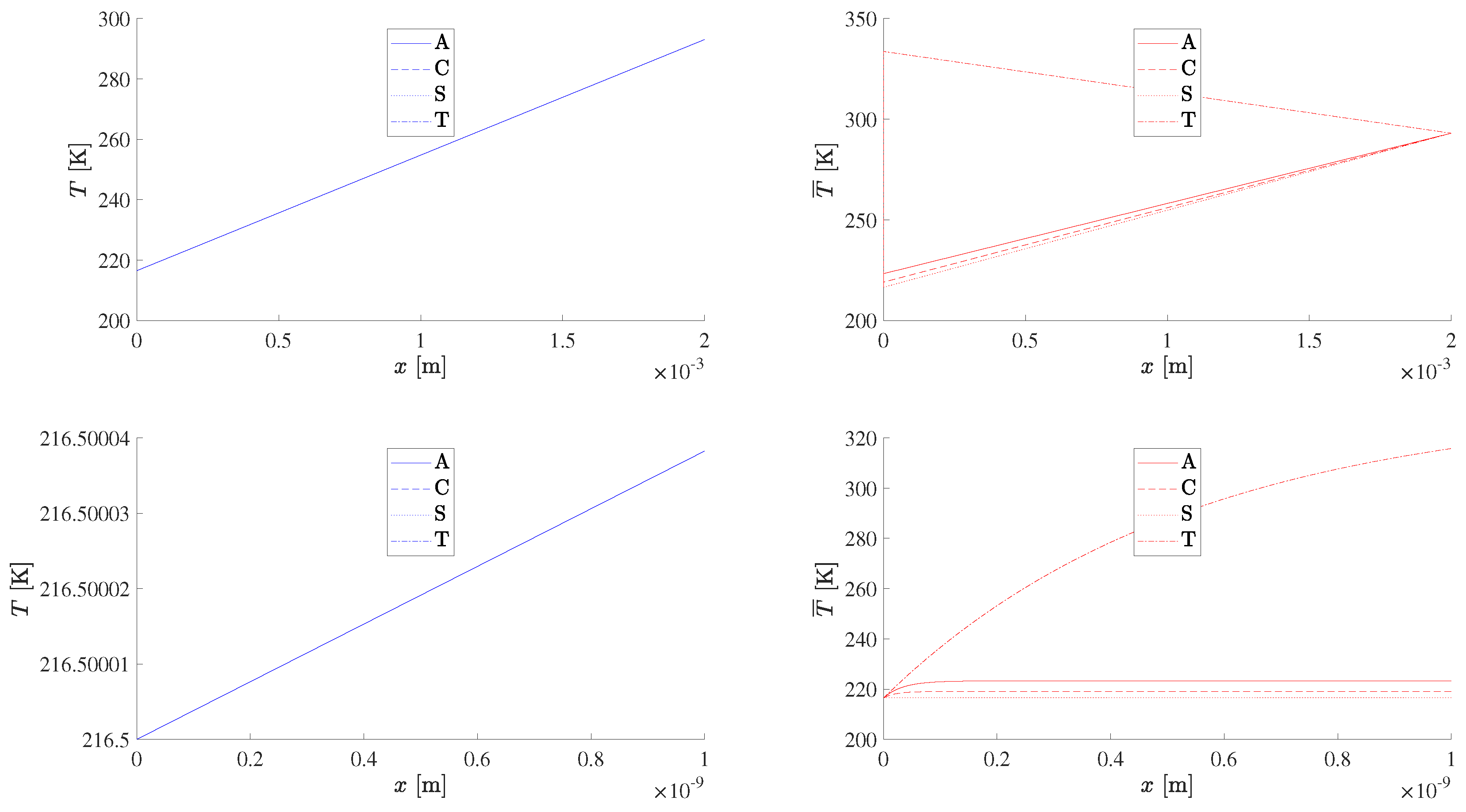
The temperature profile (49) would be linear (dotted line) between the fixed boundary values (Figure 5) in the absence of the Joule heat source due to the resistive dissipation of electric currents shown in Figure 3. The Joule heating in fair weather (left plots of Figure 5) is small enough not to affect the linear temperature profile between the temperatures (78) at the outer and (79) at the inner wall, with no discernible difference between different metals. The situation is different in a lightning storm (right plots of Figure 5): (i) the outer wall retains (bottom right of Figure 5) the same atmospheric value (78), and the intense Joule heating within the thin region of skin effect appears as a higher initial temperature $T_{\mathrm{j}}$ in Figure 5 (top right); (ii) the highest temperature $T_{\mathrm{j}}$ is for titanium, which is a heat-resistant metal, with clearly lower values for aluminium, copper and steel, in decreasing order, as shown in

Table 6. Peak temperature due to the Joule heating in the skin effect for a flight in lightning storms.

Metal	T	A	C	S	Unit
Peak temperature $T_{\mathrm{j}}$	$333.57$	$223.28$	$219.07$	$216.50$	K
Location $x_{\mathrm{j}}$	$8.32\times {10}^3$	$2.72\times {10}^2$	$1.52\times {10}^2$	$3.94$	$\times {10}^{-12}\mathrm{m}$

; (iii) Table 6 indicates the peak temperature $T_{\mathrm{j}}$ due to the Joule heating in the skin effect and the depth $x_{\mathrm{j}}$ at which it occurs for each metal, showing that the penetration depth is largest for titanium and smallest for steel, with copper and aluminium in between; (iv) outside the skin effect $x_{\mathrm{j}}\le x\le L$, the Joule heating is negligible and the temperature varies linearly from the “peak” value $T_{\mathrm{j}}$ at $x_{\mathrm{j}}$ in Table 6 to the fixed value (79) at the inner wall; (v) for all metals except titanium, the “peak” temperature $T_{\mathrm{j}}$ due to Joule heating at $x=x_{\mathrm{j}}$ is lower than the inner wall temperature $T_1>T_{\mathrm{j}}$, and thus, beyond the “peak” $x_{\mathrm{j}}\le x\le L$, the temperature rises almost linearly from $T_{\mathrm{j}}$ at $x_{\mathrm{j}}$ to $T_1$ at $x=L$. For titanium, the peak temperature $T_{\mathrm{j}}$ at $x_{\mathrm{j}}$ is larger than the inner wall temperature $T_{\mathrm{j}}>T_1$, leading to a linear decay to the same temperature (79) at the inner wall; (vi) in the full range plot (top plots of Figure 5) the temperature always ends at the inner wall value (79); (vii) the temperature always starts at the outer wall temperature (78), as is apparent for fair weather (left plots of Figure 5); (viii) for a lightning storm, the temperature also starts (right bottom plots of Figure 5) at the outer wall value (78), but, since the Joule heating region is so thin (Table 6), the temperature appears to start at $T_{\mathrm{j}}\ne T_0$ in the full thickness plot (top-right plots of Figure 5); (ix) the values of $T_{\mathrm{j}}$ are noticeably higher for titanium and close for aluminium, copper and steel (Table 6); (x) thus, over the full thickness of the slab in a lightning storm (top-right plots of Figure 5), the temperature for titanium appears higher than for fair weather, whereas, for aluminium, copper and steel, there is not much difference between fair weather and the lightning storm because the Joule heating is not too significant in either case. Thus the hierarchy is different in detail in a thin skin heating region

$$T:0\le x\le x_{\mathrm{f}}:\overline{T}>\overline{A}>\overline{C}>\overline{S}=S=C=A=T,$$

(91a)

and, overall, over the whole thickness of the slab,

$$T:0\le x_{\mathrm{f}}\le L:\overline{T}>\overline{A}\sim \overline{C}\sim \overline{S}=S=C=A=T.$$

(91b)

The hierarchy for temperature in the Joule heating region (91a) is the same as (88) for the electric and magnetic fields in a lightning storm, whereas, in fair weather, the hierarchy in (88) becomes negligible in (91a). The hierarchy over the full thickness of the slab (91b) in the top plots of Figure 5 (i) also applies to the weak Joule heating in fair weather in the skin region (bottom-left plots of Figure 5); (ii) does not show the detail (bottom-right plots of Figure 5) of more intense Joule heating in the skin region in a lightning storm (Table 6) that corresponds to the hierarchy (91b).

The heat flux (Figure 6) would be (69a)–(69b) constant (dotted line),

$$G_0=k\left(T_1-T_0\right),$$

(92)

in the absence of Joule heating. For fair weather (left plot of Figure 6), the Joule heating is very small or negligible, leading to a horizontal line for the heat flux. For a lightning storm, the Joule heating is also small outside the skin area, leading to nearly the same horizontal line as for fair weather if the full range of depth (90) is used. In order to show the effect of Joule heating in the case of a lightning storm (right plot of Figure 6), the heat flux is plotted in a subset ${10}^{-10}\mathrm{m}$ with a smaller depth within the thin skin region (89). The modulus of the heat flux is highest for copper and lowest for steel with titanium and aluminium in between in fair weather (left plot of Figure 6) when the heat flux is constant. In a lightning storm (right plot of Figure 6), in the thin region of the skin effect, the intense Joule heating leads to an increase in heat flux that is fastest for titanium and slowest for steel, with copper and aluminium in between. Thus the hierarchy for heat flux is different in a lightning storm to in fair weather,

$$G:\overline{T}>\overline{A}>\overline{C}>\overline{S}\gg C>A>T>S,$$

(93)

with much larger values in the former case. The hierarchy for the heat flux (93) is broadly similar to those for the temperature (91a)–(91b) and electric and magnetic fields (88).

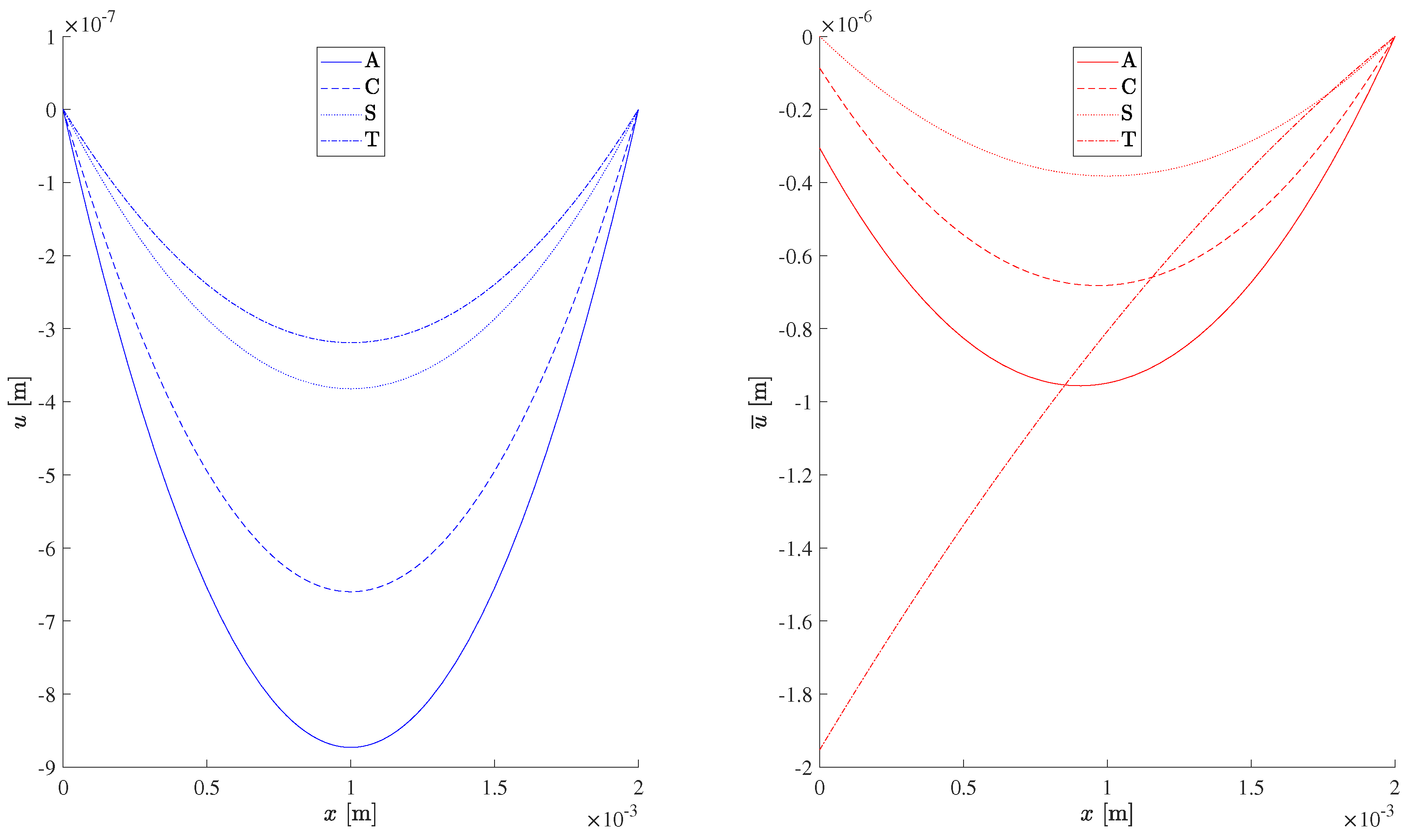
Figure 7 shows that the displacement is zero at the inner boundary and negative at the outer boundary, with larger values in modulus depending more on the metal than on the weather. The displacement is (59), the sum of a quadratic function and a negative exponential of position. The displacement in Figure 7 is close for fair weather (left) and a lightning storm (right) for all metals except titanium. In both cases, the displacement in the modulus is largest for aluminium and decreases for copper and steel. For fair weather, the smallest displacement in the modulus is for titanium:

$$\left|u\right|:\overline{A}>A>\overline{C}>C>\overline{S}>S>T.$$

(94)

For a lightning storm, the curve for titanium corresponds to a smaller displacement in modulus than for aluminium, and crosses with the curve for copper close to the outer wall, and also crosses with the curve for steel close to the inner wall. The hierarchy (94) for the displacement differs from (88) for the electric and magnetic fields (93) and from (91a)–(91b) for the temperature and (93) for the heat flux because the ordering of metals is distinct.

Figure 8 shows that the strain (60) does not vanish at either boundary and is (60) a linear function (dotted line) plus an exponential. The exponential effect away from the surface is small and the strain is almost linear, with the magnitude and slope depending more on the metal than on the weather. Although not zero, the strain is very small at the outer wall in fair weather (Figure 8, left) and increases towards the inner wall. At the inner wall, the strain in a lighting storm (Figure 8, right top) is not too different from in fair weather, starting at the outer wall with small values. The sole exception is titanium in a lightning storm, for which the strain increases rapidly in the skin region (Figure 8, right bottom), and thus, beyond the skin region (Figure 8, right top), it starts with a relatively large value and decays towards the inner wall, where it takes the lowest value after crossing with the curves for the other three metals. The hierarchy for strain

$$e_{\mathrm{xx}}:A=\overline{A}>C=\overline{C}>S=\overline{S}>T$$

(95)

is distinct from the heat flux (93), temperature (91a)–(91b) and electric and magnetic fields (88). The hierarchy for the strain (95) is similar to (94) for the modulus of the displacement interchanging fair weather and the lightning storm.

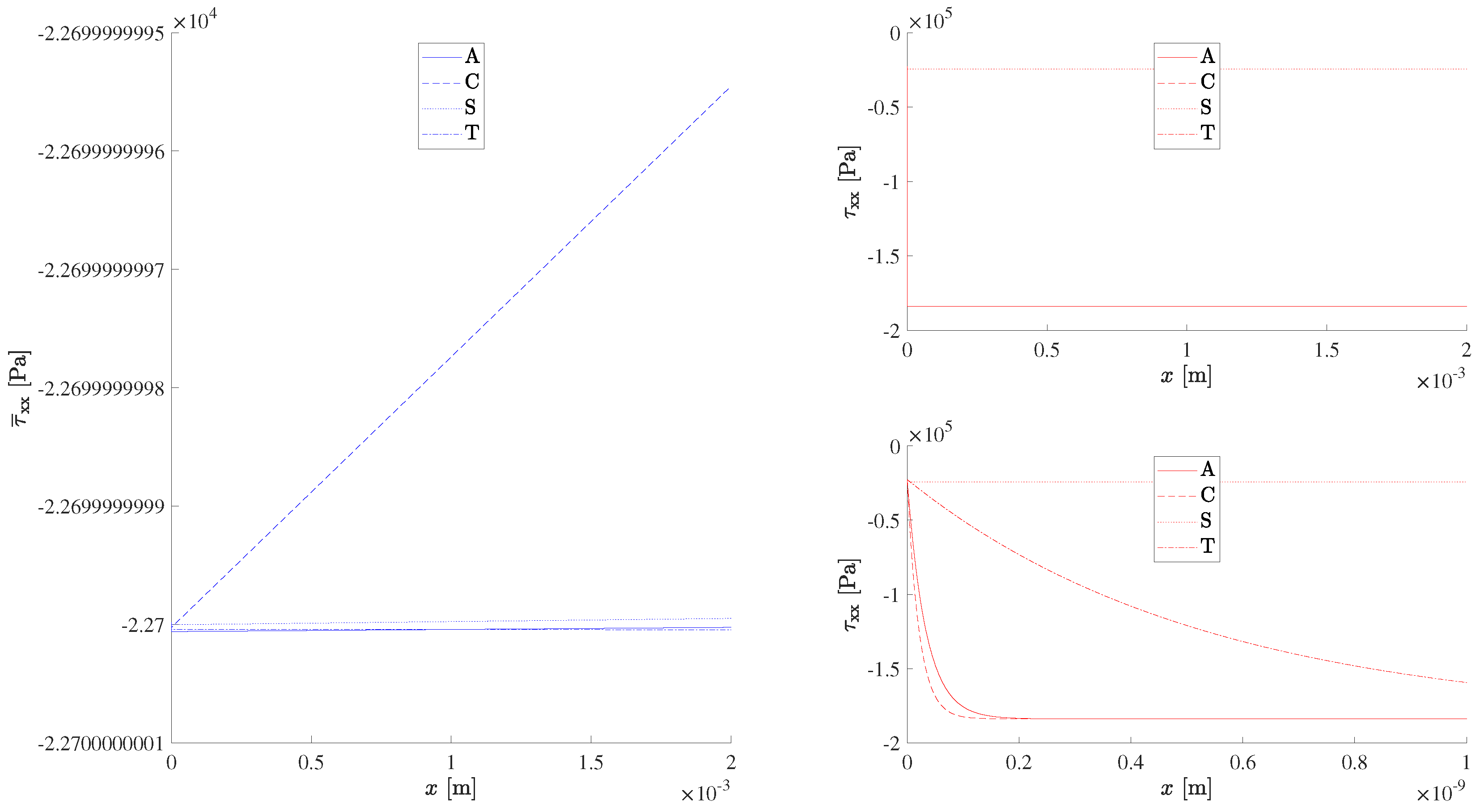
In the stress (62c), it is assumed that the reference temperature (62b) is given by the mean value of external (78) and internal (79) wall temperatures, specifying an intermediate point at about half the depth at which the thermal stresses are zero. The stress (Figure 9) equals (61) minus the atmospheric pressure at the outer boundary plus an exponential term associated with Joule heating decreasing from the outer to the inner wall and depends more on the material than on the weather. The stress starts at the atmospheric pressure at the outer wall, and, in fair weather (Figure 9, left), remains nearly constant, except for a marked linear decrease in the modulus for copper. In a lightning storm, the stress appears constant (Figure 9, right top), and smaller for steel, because, in the thin skin region (Figure 9, right bottom), the stress increases in the modulus for all metals other than steel. The hierarchy for the modulus of the stress

$$\left|{\tau }_{\mathrm{xx}}\right|:C>\overline{C}>A>\overline{A}>T>\overline{T}>\overline{S}>S,$$

(96)

is distinct from strain (95), heat flux (93), temperature (91a)–(91b) and electric and magnetic fields (88).

5. Conclusions

The main characteristics of a lightning discharge are very high voltage and very short duration, with considerable variability in observed events. Also, the way in which the high voltage is averaged over a short time can lead to a spread of values. The main input for the numerical simulation is the voltage (81), for which a range of plausible values is possible. This affects all numerical values, for example, for the strain, which would be smaller for (a) lower peak voltage; (b) longer lightning duration. It should be borne that the structural effects of a lightning discharge are very different from other unsteady phenomena, such as fatigue, for example. Fatigue involves a large number of load cycles over a long time, allowing crack propagation and growth over an increasing area. In contrast, a lightning discharge is a single short event or succession of very short events that, due to the “skin effect”, affects only a very small depth from the surface of the metal. The theory applies to a wide range of lightning voltages and durations, and, depending on the values assumed, can lead to different numerical results. The main effect on the strain comes from the thermal stresses. The choice of a reference temperature equal to the mean value of inner and outer wall temperatures minimises thermal stresses. The values of the strain in Figure 8 and Table 5 are in order of magnitude comparable to the elastic range typical for metallic alloys [22].

The numerical results show a distinction between (a) titanium on the one hand and (b) aluminium, copper and steel on the other hand, with the former exhibiting stronger electromagnetic fields, and hence greater thermoelastic effects. The following is apparent from the tables: (i) the titanium has the smallest electrical conductivity in Table 1, which is the largest electric resistivity, and hence the largest penetration depth (35c) in Table 2; (ii) although the Joule heating (42a) is comparable, the larger penetration depth leads to the highest temperature (47b) for titanium, as seen in Table 4; (iii) the titanium has the highest peak temperature in Table 6, above the inner wall temperature, in contrast with the other three metals, whose “peak” temperatures in the skin region are below the temperature at the inner wall. These conclusions are confirmed by the figures: (i) the electric and magnetic fields, respectively, in Figure 2 and Figure 4, are largest for titanium, both in fair weather (left) and in a lightning storm (right); (ii) the temperature (Figure 5) increases from the outer wall at “tropospheric” temperature to the inner wall “at room” cabin temperature, except for in the case of titanium, only for the lightning storm, where the intense Joule heating causes the highest temperature in the thin skin region; (iii) the modulus of the heat flux (Figure 6) is again highest for titanium in a lightning storm; (iv) the modulus of the displacement (Figure 7) shows a greater difference between fair weather (left) and the lightning storm (right) for titanium; (v) the strain (Figure 8) increases from negative at the outer wall to positive at the inner wall, except for in the case of titanium in a lightning storm, for which the strain reduces from the peak temperature in the skin region to the lower temperature at the inner wall; (vi) the stress (Figure 9) equals the atmospheric pressure at the outer wall, and is almost uniform on a large scale (top right), with distinct variations for different metals in the skin region (bottom right).

The basic study of aircraft flight performance and stability [23] considers an atmosphere at rest, supplemented by a vast amount of literature on the effects of adverse weather on the flight of aircraft, such as the altitude loss in wind shear [24] or the rolling motion induced by crossing wakes of other aircraft [25,26]. The effects of lightning are usually countered by the Faraday cage effect of metallic aircraft structures or by embedding conducting wires like copper in composite structures. When the electrical insulation proves insufficient, the effects of lightning are considered mostly as concerns electric and electronic equipment, which can be severely damaged or totally disabled. The present paper considers the thermomechanical effects of a lightning storm compared with flight in fair weather, requiring an approach starting with the fundamental equations of thermoelasticity and electromagnetism: (i) the constitutive equations (6a)–(6d) relating (Section 2.1) entropy, electric displacement, magnetic induction and the stress tensor to temperature, electric and magnetic fields and the strain tensor are considered; (ii) in addition to the constitutive relations based on the first principle of thermodynamics, dissipation relations (14a) (15) between electric current and energy flux, and electric field and temperature gradient (Section 2.2) are used, satisfying the second principle of thermodynamics requiring entropy growth; (iii) the constitutive and dissipative relations are used (Section 2.2) in the electromagnetic field equations (13a) and (14b), energy equation (16) and momentum equation (18); (iv) the coupled system of one scalar and three vector equations for the temperature, displacement and electric and magnetic fields are simplified (Section 2.3) for an isotropic medium in a steady state; (v) the equations are solved analytically for an infinite parallel-sided slab with dependence only along the thickness (Figure 1) with displacement orthogonal to the sides and transverse electric and magnetic fields orthogonal to each other; (vi) this specifies the dependence on the thickness of the electric field, electric current and magnetic field (Section 3.1), temperature and heat flux (Section 3.2) and displacement, strain and stress (Section 3.3); (vii) the results are used to compare flight at the tropopause in fair weather (Section 4.2) and a lightning storm (Section 4.3) for a slab of four metals, namely, aluminium, copper, steel and titanium (Section 4.1).

References

1. Love, A.E.H. A Treatise on the Mathematical Theory of Elasticity, 4th ed.; Dover Publications, Inc.: New York, NY, USA, 1944. [Google Scholar]
2. Timoshenko, S.P.; Goodier, J.N. Theory of Elasticity, 2nd ed.; Engineering Societies Monographs; McGraw-Hill Book Company: New York, NY, USA, 1951. [Google Scholar]
3. Cady, W.G. Piezoelectricity: An Introduction to the Theory and Applications of Electromechanical Phenomena in Crystals, 1st ed.; International Series in Pure and Applied Physics; McGraw-Hill Book Company, Inc.: New York, NY, USA, 1946. [Google Scholar]
4. Woodson, H.H.; Melcher, J.R. Elastic and Fluid Media. In Electromechanical Dynamics; John Wiley & Sons, Inc.: New York, NY, USA, 1968; Volume 3. [Google Scholar]
5. Eringen, A.C.; Maugin, G.A.M. Electrodynamics of Continua I: Foundations and Solid Media; Springer-Verlag: New York, NY, USA, 1990. [Google Scholar]
6. Trindade, M.A.; Benjeddou, A. Effective Electromechanical Coupling Coefficients of Piezoelectric Adaptive Structures: Critical Evaluation and Optimization. Mech. Adv. Mater. Struct. 2009, 16, 210–223. [Google Scholar] [CrossRef]
7. Sun, J.; Guan, Q.; Liu, Y.; Leng, J. Morphing aircraft based on smart materials and structures: A state-of-the-art review. J. Intell. Mater. Syst. Struct. 2016, 27, 2289–2312. [Google Scholar] [CrossRef]
8. Stratton, J.A. Electromagnetic Theory; International Series in Pure and Applied Physics; McGraw-Hill Book Company, Inc.: New York, NY, USA, 1941. [Google Scholar]
9. Campos, L.M.B.C. Linear Differential Equations and Oscillators, 1st ed.; Mathematics and Physics for Science and Technology; CRC Press: Boca Raton, FL, USA, 2019; Volume 4. [Google Scholar] [CrossRef]
10. Campos, L.M.B.C.; Moleiro, F.A.M.; Silva, M.J.S. On the fundamental equations of unsteady anisothermal viscoelastic piezoelectromagnetism. Eur. J. Mech.-A/Solids 2019, 78, 103848. [Google Scholar] [CrossRef]
11. Carslaw, H.S.; Jaeger, J.C. Conduction of Heat in Solids, 2nd ed.; Oxford Science Publications; Oxford University Press: Oxford, UK, 1959. [Google Scholar]
12. Jackson, J.D. Classical Electrodynamics, 3rd ed.; John Wiley & Sons, Inc.: New York, NY, USA, 1999. [Google Scholar]
13. Campos, L.M.B.C.; Vilela, L.A.R. Vector Fields with Applications to Thermodynamics and Irreversibility, 1st ed.; Mathematics and Physics for Science and Technology; CRC Press: Boca Raton, FL, USA, 2022; Volume 5. [Google Scholar]
14. Schouten, J.A. Tensor Analysis for Physicists, 2nd ed.; Clarendon Press: Oxford, UK, 1954. [Google Scholar]
15. Campos, L.M.B.C. Complex Analysis with Applications to Flows and Fields, 1st ed.; Mathematics and Physics for Science and Technology; CRC Press: Boca Raton, FL, USA, 2011; Volume 1. [Google Scholar] [CrossRef]
16. Lide, D.R. (Ed.) CRC Handbook of Chemistry and Physics, 82nd ed.; CRC Press: Boca Raton, FL, USA, 2001. [Google Scholar]
17. Avallone, E.A.; Baumeister, T., III (Eds.) Marks’ Standard Handbook for Mechanical Engineers, 10th ed.; McGraw-Hill Professional: New York, NY, USA, 1996. [Google Scholar]
18. Perkins, C.D.; Hage, R.E. Airplane Performance: Stability and Control; John Wiley & Sons, Inc.: New York, NY, USA, 1960. [Google Scholar]
19. Etkin, B.; Reid, L.D. Dynamics of Flight: Stability and Control, 3rd ed.; John Wiley & Sons, Inc.: New York, NY, USA, 1995. [Google Scholar]
20. Schonland, B.F.J. Atmospheric Electricity, 2nd ed.; Methuen’s Monographs on Physical Subjects; Methuen & Co. Ltd.: London, UK, 1953. [Google Scholar]
21. Watt, A.D. ELF electric fields from thunderstorms. J. Res. Natl. Bur. Stand. Sect. D Radio Propag. 1960, 64, 425–433. [Google Scholar] [CrossRef]
22. Ju, H.; Lin, C.; Tian, Y.; Liu, Z.; Jiang, H.; Sun, D. Mechanical Properties Study of Fe-Mn-Si Shape Memory Alloys Welding Seam Formed by Laser Welding with Filler Powder. Materials 2018, 11, 1454. [Google Scholar] [CrossRef] [PubMed]
23. Miele, A. Flight Mechanics, 1st ed.; Addison-Wesley Publishing Company: Reading, MA, USA, 1962; Volumes 1–2. [Google Scholar]
24. Campos, L.M.B.C. On a pitch control law for a constant glide slope through windshears. Aeronaut. J. 1989, 93, 290–300. [Google Scholar] [CrossRef]
25. Gerz, T.; Holzäpfel, F.; Darracq, D. Commercial aircraft wake vortices. Prog. Aerosp. Sci. 2002, 38, 181–208. [Google Scholar] [CrossRef]
26. Nelson, R.C.; Jumper, E.J. Aircraft Wake Vortices and Their Effect on Following Aircraft. In Proceedings of the AIAA Atmospheric Flight Mechanics Conference and Exhibit, Montréal, QC, USA, 6–9 August 2001. [Google Scholar] [CrossRef]
Figure 1. Formulation of the problem of piezoelectromagnetism in a parallel-sided slab: (i) the electric and magnetic fields are orthogonal to each other and both parallel to the sides of the slab; (ii) the Ohmic electric current is parallel to the electric field and hence the magnetic force is orthogonal to the sides of the slab; (iii) the electric field vector has zero divergence, so there is no electric charge and no electric force; (iv) the displacement vector is orthogonal to the sides of the slab, and, since it depends only on the orthogonal coordinate x, as for all other variables, the non-zero components of the strain and stress are, respectively, e xx and τ xx . The problem has a unique solution with the following boundary conditions at the surface of the slab: (a) on the external, atmospheric side, the electric field, temperature and pressure; (b) on the internal, cabin side, the temperature and displacement.
Applsci 15 03605 g001
Figure 2. Electric field along the initial part of the slab using (68) with penetration depth l in Table 2 and surface electric field: (left) for fair weather (80); (right) for a lightning storm (82).
Applsci 15 03605 g002
Figure 3. Electric current along the initial part of the slab using (68) with penetration depth l from Table 2 and Ohmic electrical conductivity χ in Table 1, with surface electric current for (left) fair weather; (right) lightning storm.
Applsci 15 03605 g003
Figure 4. Magnetic field along the initial part of the slab using (68) with penetration depth l from Table 2 and dielectric permittivity ε and magnetic susceptibility μ from Table 1, with surface magnetic field for (left) fair weather; (right) a lightning storm.
Applsci 15 03605 g004
Figure 5. Temperature along the entire slab with length (90) (top plots) and along the initial part of the slab (bottom plots) in fair weather (left) and lightning storm (right) cases using (49) and (47b) with outer T 0 and inner T 1 boundary temperatures from Table 3, penetration depth l from Table 2 and heating function at the surface Q 0 from Table 4.
Applsci 15 03605 g005
Figure 6. Heat flux along the entire slab with thickness (90), using (50b) and (47b), with the same values of l, T 0 , T 1 and Q 0 as in Figure 5.
Applsci 15 03605 g006
Figure 7. Displacement along the entire slab with thickness (90), for (left) fair weather or (right) a lightning storm, using (59), with penetration depth l from Table 2 and parameters a , b , f from Table 4.
Applsci 15 03605 g007
Figure 8. Strain along the entire slab with thickness (90), for (left) fair weather or (right) a lightning storm, using (60) with the same values of the parameters l , a , b , f as in Figure 6.
Applsci 15 03605 g008
Figure 9. Stress along the entire slab with thickness (90), using (61) with surface electric field (80) for fair weather (left) or (82) for a lightning storm (right), with penetration depth l from Table 2, atmospheric pressure p 0 from Table 3 and dielectric permittivity ε and magnetic permeability μ from Table 1.
Applsci 15 03605 g009