Numerical Simulation of Flexural Deformation Through an Integrated Cosserat Expanded Constitutive Model and the Drucker–Prager Criterion

Abstract

In this article, we propose a new numerical approach, abbreviated as Cos-SDA, for analyzing flexural deformation problems of geomaterials. The Cos-SDA is achieved by implanting the strong discontinuity approach (SDA) into the computational framework of the Cosserat continuum finite element approach (Cos-FEA). Most of the Cos-FEA is based on the Mohr–Coulomb (M-C) criterion at present. However, the M-C yield surface is not smooth because of hexagonal corners, which can cause numerical difficulties in the Cos-FEA. The Drucker–Prager (D-P) criterion can be viewed as a smooth approximation to the M-C criterion. Meanwhile, the M-C criterion does not take into account the influence of the intermediate principal stress on strength, but D-P criterion is able to reflect the combined effect of the three principal stresses. Therefore, based on the MATLAB system, an improved three-dimensional (3D) Cos-FEA is proposed by using the D-P criterion. Through a numerical example of three-dimensional flexural deformation analysis of an excavation in layered rock, it is demonstrated that the improved Cos-FEA can effectively simulate flexural deformation and the entire progressive failure process. The improved Cos-FEA inherits the advantages of both the Cos-FEA and D-P criterion and neutralizes their mechanical responses, so it is more reasonable in simulating the progressive failure process occurring in an alternating rock mass. Most importantly, the D-P criterion-based Cos-FEA is observed to have a higher convergence speed and stability.

1. Introduction

The Cosserat continuum theory is superior to the classical continuum theory (without an internal length parameter) to describe the mechanical behaviors of materials within their micro-structure. It has become a hot topic and has increasingly caught the attention of many researchers. The Cosserat continuum model, an asymmetrical elastic theory for layered rocks with bending stiffness, was first proposed by the Cosserat brothers [1] at the beginning of the past century. In the proposed theory, the influence of defined characteristic length of the material was considered by introducing the concepts of couple stress and bending curvature. The stress tensor and strain tensor in the Cosserat continuum theory are generally not symmetric, and the difference in the shear components of stress is equilibrated by micromoments. When the characteristic length of the medium is regarded as infinitesimal, the Cosserat continuum would degenerate as the classical continuum. Marin, Alavi, Tummers, Ghiba and their co-workers [2,3,4,5,6,7] have extensively developed the Cosserat theory in relation to layered materials.

A new 3D Cosserat expanded constitutive model [8] is based on the macro-average significance, in which the influence of bending was taken into account. In this model, a new unit cell, namely the material point containing two alternate layers, was employed to simulate the coordination of the meso-displacement between two layers with mismatched mechanical properties. This model provides a new way for analyzing the deformation and failure of layered rock. Firstly, using the elastic model and having the Cosserat stresses, namely the macro-average ones, which have been determined, the conventional stresses of the different layers in a unit cell could be obtained in sequence. Then, the conventional stresses could be utilized through a routine way for strength and failure analysis.

Figure 1 shows the schematic of the stress components of the three-dimensional Cosserat continuum on an alternating layered rock mass. For the derivation of the 3D Cosserat expanded constitutive model in relation to the layered materials, the following assumptions are made:

• The alternating layered medium is composed of a medium bonding different mechanical properties, and the bonding properties of the interface of every layered medium is good. There is no sliding, opening or embedding between them.
• When subjected to deformations of stretching and bending, four side faces of the block element maintain the plane (Plane Section Assumption).
• The material strain is very small (Small Deformation Assumption).

Since the 1980s, the Cosserat theory has been applied to geotechnical engineering. Adhikary [9], Mühlhaus [10], SHE [11], LI [12] and their co-workers have conducted a substantial amount of work to verify the theory, especially for bedded rock masses. The results indicated that Cosserat medium method was better and more applicable to simulate failure features for a bedded rock mass with slipping and bending deformations. Based on the classical Cosserat medium theory for jointed rocks, LI et al. established a new 2D and 3D Cosserat expanded constitutive model for bedded salt rocks [13,14,15,16,17,18].

It is well known that there are many criteria in geomechanics [19,20,21,22]. The M-C and D-P criteria are applied widely among them. The M-C criterion hexagonal yield surface is not smooth but has corners. These corners of the hexagon can cause numerical computation difficulty in its application to Cosserat elasto-plastic analysis. In order to improve convergence, many researchers have suggested using the rounded edges and vertices for approximating the M-C criterion. Among them, one of the most extensive is the D-P strength criterion, and it can be seen as the M-C criterion used in order to avoid the difficulties of smoothing approximation. Moreover, the Cos-FEA is currently written by using the M-C criterion (e.g., in References [23,24,25,26,27]). However, the D-P strength criterion in the analysis of underground excavation also occupies a very important position, as what kind of strength criterion can be applied to the Cosserat model that has a better applicability in inter-bedded rocks? Therefore, it is necessary to study it.

In this study, a full 3D Cos-FEA based on the D-P criterion is presented in the small deformation framework. The mathematical formulation follows the general framework proposed. Following the Introduction, in Section 2, Cosserat continuum expanded constitutive equations are discussed. Section 3 provides a set of finite element expressions of the Cosserat continuum. Section 4 explores the mechanics and the three-dimensional Cosserat constitutive equations. Section 5 presents modified yield criteria in the Cosserat medium theory. In Section 6, the elasto-plastic finite element codes for the Cosserat expanded constitutive model and classical continuum model were developed using MATLAB (R2020a). In Section 7, the examples concern cantilever layered plate structures with various geometries and boundary conditions for which an analytical solution or an approximation to the analytical solution is available. This example demonstrates the accuracy of the Cos-FEA. Finally, the model is applied to the deformation and stability analysis of an excavation in layered rock, and the results are compared to the predictions of the traditional FEM for the follow-up study on the strength criterion of the Cosserat model to provide some suggestions and references.

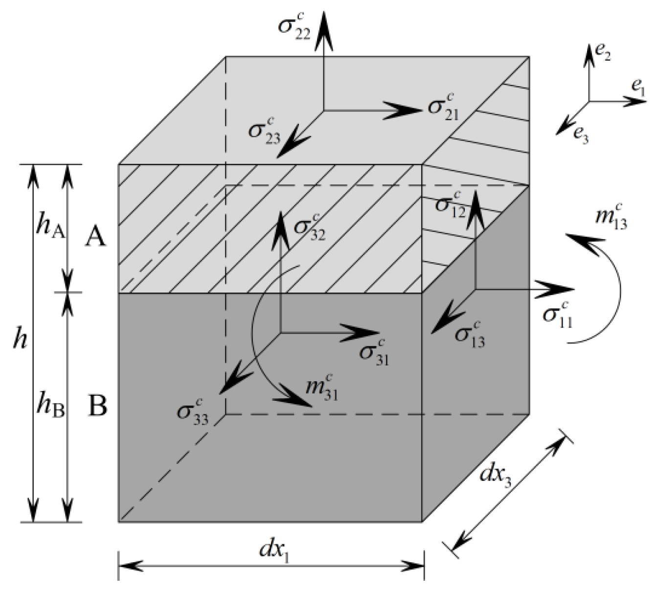
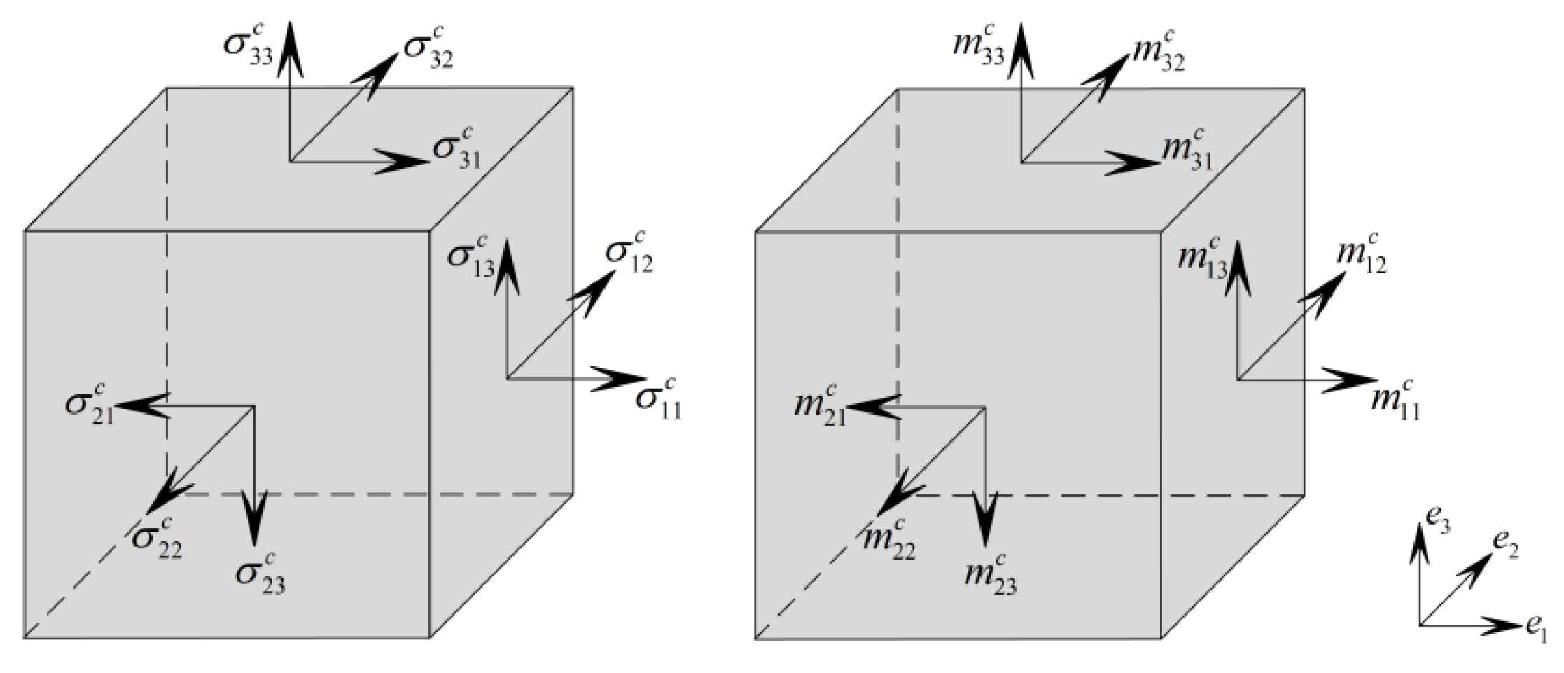
2. Basics of the Cosserat Continuum Theory

Micropolar or Cosserat theory assumes that micromoments exist at each point of the continuum. In the Cosserat theory, the equilibrium of forces and equilibrium of moments are expressed in the following form [11]:

$${\sigma }_{ij,i}+b_j=0$$

(1)

$$m_{kj,j}+e_{kij}{\sigma }_{ij}+{\nu }_k=0$$

(2)

where σ is the Cosserat stress, b is the body force, e is the permutation operator, m is the Cosserat couple stress, and ν is the body couple moment. The stress component σ_ij is analogous with stress of the classical continuum theory, which means the projection of the intensity of force on the j-axis on the cross-section is normal to the i-axis. Figure 2 shows the representation of the stress and couple stress components in the 3D Cosserat continuum theory. For the stresses, the first subscript of the letter represents the direction perpendicular to which the stress is loaded, and the second subscript indicates the direction in which the stress is actually loaded. For the bending stress, the first subscript of the letter means the axis around which the bending stress is loaded, and the second subscript also indicates the direction in which the bending stress is loaded. The symbols of the components of the stress tensor are similar to the standard symbols used in the classical continuum theory. However, it differs from the notation used in some of the previous papers on the Cosserat theory, for example, References [2,3,4,5,6,7,8,9,10].

In the absence of a couple moment, Equation (2) reduces to the following from [28]:

$$e_{kij}{\sigma }_{ij}=0$$

(3)

Equation (3) demonstrates that the symmetry between stress and its work-conjugate strain measure is maintained. Additionally, the Cosserat continuum simplifies to the classical continuum under these conditions. The symmetry of the stress and strain tensors also introduces a minor symmetry in the elasticity tensor. The definitions of stress and moment traction are provided as follows:

$$\left\{\begin{array}{l}{t}_{\sigma }=\sigma n\hfill \\ t_m=\mu n\hfill \end{array}\right.$$

(4)

where n is the normal vector of the surface in the current coordinates.

3. Finite Element Expressions

The difference between the Cosserat and classical FEAs are the strain transformation matrix, B, stiffness matrix, D, and degrees of freedom at each node.

In the Cos-FEA formulation, each node is associated with three displacements or three rotational degrees of freedom. The vector of the i-th node degrees of freedom is defined as:

$${[u^c{\omega }^c]}_i={[u_1^c, u_2^c, u_3^c, {\omega }_1^c, {\omega }_2^c, {\omega }_3^c]}_i^T$$

(5)

Using a notation similar to Voigt notation, the second-order strain and curvature tensors can be expressed in the following vectorial form:

$$\left\{\begin{array}{l}{\epsilon }^c={\left[{\epsilon }_{11}^c{\epsilon }_{22}^c{\epsilon }_{33}^c{\epsilon }_{12}^c{\epsilon }_{21}^c{\epsilon }_{32}^c{\epsilon }_{23}^c{\epsilon }_{13}^c\right]}^T\hfill \\ {\kappa }^c={\left[{\kappa }_{13}^c{\kappa }_{31}^c\right]}^T\hfill \end{array}\right.$$

(6)

Finally, by employing Finite Element Method (FEM) discretization techniques along with the interpolation function, N, the strain and curvature fields can be interpolated in relation to the nodal degrees of freedom vectors u_i^c and ω_i^c as follows:

$$\left\{\begin{array}{c}\epsilon \\ \kappa \end{array}\right\}=B_i\left\{\begin{array}{c}{u}_i^c\\ {\omega }_i^c\end{array}\right\}$$

(7)

The operator B_i has a block structure and is expressed in the following form:

$$B_i=\left(\begin{array}{cc}{B}_{i1}& B_{i2}\\ 0_{2\times 3}& B_{i3}\end{array}\right)$$

(8)

with

$$B_{i1}=\left[\begin{array}{ccc}{N}_{i,1}& 0& 0\\ 0& N_{i,2}& 0\\ 0& 0& N_{i,3}\\ 0& N_{i,1}& 0\\ N_{i,2}& 0& 0\\ 0& N_{i,3}& 0\\ 0& 0& N_{i,2}\\ 0& 0& N_{i,1}\end{array}\right], B_{i2}=\left[\begin{array}{ccc}0& 0& 0\\ 0& 0& 0\\ 0& 0& 0\\ 0& 0& -N_i\\ 0& 0& N_i\\ N_i& 0& 0\\ -N_i& 0& 0\\ 0& N_i& 0\end{array}\right], \mathrm{and} B_{i3}={\left[\begin{array}{cc}{N}_{i,3}& 0\\ 0& 0\\ 0& N_{i,1}\end{array}\right]}^T$$

(9)

where N_i represents the shape function associated with the i-th node. Additionally, N_i is utilized for interpolating both the displacement and rotation fields.

In the context of small deformation analysis, the internal force F^int is defined as:

$$F^{\mathrm{int}}={\displaystyle {\int }_V(B_{i1}^T\sigma +B_{i2}^T\sigma +B_{i2}^{T}m)}dv$$

(10)

Finally, in the interlayer material stiffness analysis, the stiffness matrix K_ij is defined as:

$$K_{ij}=B_i^{T}D{B}_j$$

(11)

where D is a block symmetric matrix that establishes the relationship between the stress and couple stress measures and their work-conjugate measures, namely strains and curvatures, through appropriate constitutive laws D₁ and D₂. In the local coordinate system, indicated by the hat symbol, ^, the constitutive laws are expressed as:

$$\left\{\begin{array}{c}\widehat{\sigma }\\ \widehat{m}\end{array}\right\}=\widehat{D}\left\{\begin{array}{c}\widehat{\epsilon }\\ \widehat{\kappa }\end{array}\right\}=\left[\begin{array}{cc}{\widehat{D}}_1& 0_{8\times 2}\\ 0_{2\times 8}& {\widehat{D}}_2\end{array}\right]\left\{\begin{array}{c}\widehat{\epsilon }\\ \widehat{\kappa }\end{array}\right\}$$

(12)

In three-dimensional analysis, in order to obtain the D₁ and D₂ in the global coordinate system, a transformation matrix L should be applied to both ${\widehat{D}}_1$ and ${\widehat{D}}_2$. It is expressed in the following form:

$$D=\left[\begin{array}{cc}{D}_1& 0_{8\times 2}\\ 0_{2\times 8}& D_2\end{array}\right]=L^T\widehat{D}L=\left[\begin{array}{cc}{L}_1^T{\widehat{D}}_1{L}_1& 0_{8\times 2}\\ 0_{8\times 2}& L_2^T{\widehat{D}}_2{L}_2\end{array}\right]$$

(13)

with

$$L=\left[\begin{array}{cc}{L}_1& 0_{8\times 2}\\ 0_{2\times 8}& L_2\end{array}\right],L_1=\left[\begin{array}{cccc}\lambda & & & \\ & \lambda & & \\ & & \lambda & \\ & & & \lambda \end{array}\right],\mathrm{and}{L}_2=\lambda =\left[\begin{array}{cc}\cos \theta & \sin \theta \\ -\sin \theta & \cos \theta \end{array}\right]$$

(14)

where θ is the included angle between the global coordinate system and the local coordinate system.

Using Equations (11) and (12), the material stiffness matrix K_ij is expressed in the following form:

$$K_{ij}=B_i^{T}D{B}_j=\left(\begin{array}{cc}{B}_{i1}^T{D}_1{B}_{j1}& B_{i1}^T{D}_1{B}_{j2}\\ B_{i2}^T{D}_1{B}_{j1}& B_{i2}^T{D}_2{B}_{j2}+B_{i3}^T{D}_2{B}_{j3}\end{array}\right)$$

(15)

4. Three-Dimensional Cosserat Constitutive Equations

The global three-dimensional Cosserat constitute relationship for the composite material is obtained [29,30]:

$$\left\{\begin{array}{c}{\sigma }^c\\ m^c\end{array}\right\}=D\left\{\begin{array}{c}{\epsilon }^c\\ {\kappa }^c\end{array}\right\}=C^{-1}\left\{\begin{array}{c}{\epsilon }^c\\ {\kappa }^c\end{array}\right\}$$

(16)

or

$$\left\{\begin{array}{c}{\sigma }_{11}^c\\ {\sigma }_{22}^c\\ {\sigma }_{33}^c\\ {\sigma }_{12}^c\\ {\sigma }_{21}^c\\ {\sigma }_{32}^c\\ {\sigma }_{23}^c\\ {\sigma }_{13}^c\\ m_{13}^c\\ m_{31}^c\end{array}\right\}={\left[\begin{array}{cccccccccc}{C}_{11}& C_{12}& C_{13}& 0& 0& 0& 0& 0& 0& 0\\ & C_{22}& C_{23}& 0& 0& 0& 0& 0& 0& 0\\ & & C_{33}& 0& 0& 0& 0& 0& 0& 0\\ & & & C_{44}& C_{45}& 0& 0& 0& 0& 0\\ & & & & C_{55}& 0& 0& 0& 0& 0\\ & & & & & C_{44}& C_{45}& 0& 0& 0\\ & & & & & & C_{55}& 0& 0& 0\\ & & sym& & & & & C_{66}& 0& 0\\ & & & & & & & & C_{77}& 0\\ & & & & & & & & & C_{88}\end{array}\right]}^{-1}\left\{\begin{array}{c}{\epsilon }_{11}^c\\ {\epsilon }_{22}^c\\ {\epsilon }_{33}^c\\ {\epsilon }_{12}^c\\ {\epsilon }_{21}^c\\ {\epsilon }_{32}^c\\ {\epsilon }_{23}^c\\ {\epsilon }_{13}^c\\ {\kappa }_{13}^c\\ {\kappa }_{31}^c\end{array}\right\}$$

(17)

where

$$\left\{\begin{array}{l}{C}_{11}={\displaystyle \frac{\frac{{\alpha }_{\mathrm{A}}{E}_{\mathrm{A}}}{1-{\nu }_{\mathrm{A}}^2}+\frac{{\alpha }_{\mathrm{B}}{E}_{\mathrm{B}}}{1-{\nu }_{\mathrm{B}}^2}}{\left(\frac{{\alpha }_{\mathrm{A}}{E}_{\mathrm{A}}}{1-{\nu }_{\mathrm{A}}}+\frac{{\alpha }_{\mathrm{B}}{E}_{\mathrm{B}}}{1-{\nu }_{\mathrm{B}}}\right)\left(\frac{{\alpha }_{\mathrm{A}}{E}_{\mathrm{A}}}{1+{\nu }_{\mathrm{A}}}+\frac{{\alpha }_{\mathrm{B}}{E}_{\mathrm{B}}}{1+{\nu }_{\mathrm{B}}}\right)}}\hfill \\ C_{12}=-{\displaystyle \frac{\frac{{\alpha }_{\mathrm{A}}{\nu }_{\mathrm{A}}}{1-{\nu }_{\mathrm{A}}}+\frac{{\alpha }_{\mathrm{B}}{\nu }_{\mathrm{B}}}{1-{\nu }_{\mathrm{B}}}}{\frac{{\alpha }_{\mathrm{A}}{E}_{\mathrm{A}}}{1-{\nu }_{\mathrm{A}}}+\frac{{\alpha }_{\mathrm{B}}{E}_{\mathrm{B}}}{1-{\nu }_{\mathrm{B}}}}}=-{\displaystyle \frac{{\alpha }_{\mathrm{A}}{\nu }_{\mathrm{A}}(1-{\nu }_{\mathrm{B}})+{\alpha }_{\mathrm{B}}{\nu }_{\mathrm{B}}(1-{\nu }_{\mathrm{A}})}{{\alpha }_{\mathrm{A}}{E}_{\mathrm{A}}(1-{\nu }_{\mathrm{B}})+{\alpha }_{\mathrm{B}}{E}_{\mathrm{B}}(1-{\nu }_{\mathrm{A}})}}\hfill \\ C_{13}=-{\displaystyle \frac{\frac{{\alpha }_{\mathrm{A}}{\nu }_{\mathrm{A}}{E}_{\mathrm{A}}}{1-{\nu }_{\mathrm{A}}^2}+\frac{{\alpha }_{\mathrm{B}}{\nu }_{\mathrm{B}}{E}_{\mathrm{B}}}{1-{\nu }_{\mathrm{B}}^2}}{\left(\frac{{\alpha }_{\mathrm{A}}{E}_{\mathrm{A}}}{1-{\nu }_{\mathrm{A}}}+\frac{{\alpha }_{\mathrm{B}}{E}_{\mathrm{B}}}{1-{\nu }_{\mathrm{B}}}\right)\left(\frac{{\alpha }_{\mathrm{A}}{E}_{\mathrm{A}}}{1+{\nu }_{\mathrm{A}}}+\frac{{\alpha }_{\mathrm{B}}{E}_{\mathrm{B}}}{1+{\nu }_{\mathrm{B}}}\right)}}\hfill \\ C_{22}={\displaystyle \frac{{\alpha }_{\mathrm{A}}}{E_{\mathrm{A}}}}+{\displaystyle \frac{{\alpha }_{\mathrm{B}}}{E_{\mathrm{B}}}}-{\displaystyle \frac{2{\alpha }_{\mathrm{A}}{\alpha }_{\mathrm{B}}}{E_{\mathrm{A}}{E}_{\mathrm{B}}}}{\displaystyle \frac{{({\nu }_{\mathrm{A}}{E}_{\mathrm{B}}-{\nu }_{\mathrm{B}}{E}_{\mathrm{A}})}^2}{[{\alpha }_{\mathrm{A}}{E}_{\mathrm{A}}(1-{\nu }_{\mathrm{B}})+{\alpha }_{\mathrm{B}}{E}_{\mathrm{B}}(1-{\nu }_{\mathrm{A}})]}}\hfill \\ C_{23}=C_{12}, C_{33}=C_{11}\hfill \\ C_{44}={\left({\alpha }_{\mathrm{A}}{\displaystyle \frac{4G_{\mathrm{A}}{G}_{\mathrm{A}}^c}{G_{\mathrm{A}}+G_{\mathrm{A}}^c}}+{\alpha }_{\mathrm{B}}{\displaystyle \frac{4G_{\mathrm{B}}{G}_{\mathrm{B}}^c}{G_{\mathrm{B}}+G_{\mathrm{B}}^c}}\right)}^{-1}\hfill \\ C_{45}=C_{44}\left({\alpha }_{\mathrm{A}}{\displaystyle \frac{G_{\mathrm{A}}^c-G_{\mathrm{A}}}{G_{\mathrm{A}}+G_{\mathrm{A}}^c}}+{\alpha }_{\mathrm{B}}{\displaystyle \frac{G_{\mathrm{B}}^c-G_{\mathrm{B}}}{G_{\mathrm{B}}+G_{\mathrm{B}}^c}}\right)\hfill \\ C_{55}=C_{44}, C_{66}={\displaystyle \frac{1}{2({\alpha }_{\mathrm{A}}{G}_{\mathrm{A}}+{\alpha }_{\mathrm{B}}{G}_{\mathrm{B}})}}\hfill \\ C_{77}=C_{88}={\left[{\displaystyle \frac{{\alpha }_{\mathrm{A}}^3{E}_{\mathrm{A}}{h}^2}{12}}+{\displaystyle \frac{{\alpha }_{\mathrm{B}}^3{E}_{\mathrm{B}}{h}^2}{12}}+{\displaystyle \frac{{\alpha }_{\mathrm{A}}{\alpha }_{\mathrm{B}}{E}_{\mathrm{A}}{E}_{\mathrm{B}}{h}^2}{4\left({\alpha }_{\mathrm{A}}{E}_{\mathrm{A}}+{\alpha }_{\mathrm{B}}{E}_{\mathrm{B}}\right)}}\right]}^{-1}\hfill \end{array}\right.$$

(18)

where E is the modulus of elasticity, ν is the Poisson ratio, G is the shear modulus, and G^c is the Cosserat second shear modulus. α is the volume ratio, a_A = h_A/h, a_B = h_B/h, h = h_A + h_B. The subscript letter indicates layer A or B.

5. Modified Yield Criteria in Cosserat Medium Theory

The yield function is expressed by three invariants of the stress deviator tensors I₁, J₂ and J₃ in the classical continuum theory. The criterion can be written in the general form

$$F\left({\sigma }_{ij},\gamma \right)=f\left(I_1,J_2,J_3,\gamma \right)\le 0$$

(19)

where γ is an internal variable characterizing the isotropic hardening or softening behavior of the material.

In the Cosserat continuum theory, the strain tensor and the stress tensor exhibit asymmetric properties, which makes the classical yield criterion unable to be directly applied to the Cosserat continuum. In view of this, the application of the M-C yield criterion in an extended constitutive model based on the Cosserat theory was discussed.

In this case, the Cosserat strain tensor will be divided into two parts, symmetry and asymmetry [26]:

$$\left\{\begin{array}{l}{\epsilon }_{ij}^{sym}=(u_{j,i}+u_{i,j})/2,{\kappa }_{i3}={\omega }_{,i}^c\hfill \\ {\epsilon }_{ij}^{ant}=(u_{j,i}-u_{i,j})/2+e_{ij}{\omega }^c\hfill \end{array}\right.$$

(20)

where e_ij is the alternating tensor, and “sym” and “ant” of the superscript denote symmetry and skew symmetry, respectively.

Similarly, the Cosserat stress tensor will be divided into two parts, i.e., symmetry and asymmetry:

$$\left\{\begin{array}{l}{\sigma }_{ij}^{sym}=D_{ijkl}^{sym}{\epsilon }_{kl}^{sym}\hfill \\ {\sigma }_{ij}^{ant}=(D_{ijkl}-D_{ijkl}^{sym}){\epsilon }_{kl}^{ant}\hfill \\ m_{i3}=B_i{\kappa }_{i3}\hfill \end{array}\right.$$

(21)

where D_ijkl and B_i are material stiffness tensors.

By using symmetrical and skew-symmetric stress tensors, three invariant expressions of the stress deviator tensors I₁, J₂ and J₃ are modified in the classical continuum theory. From Equation (21), we obtain

$$\left\{\begin{array}{l}{I}_1={\sigma }_{11}+{\sigma }_{22}+{\sigma }_{33}\hfill \\ J_2=J_2^{sym}+J_2^{ant}+J_2^m\hfill \\ J_3=s_{11}^{sym}{s}_{22}^{sym}{s}_{33}^{sym}-s_{12}^{sym}{s}_{21}^{sym}{s}_{33}^{sym}\hfill \end{array}\right.$$

(22)

where

$$\left\{\begin{array}{l}\begin{array}{l}{J}_2^{sym}=[{(s_{11}^{sym})}^2+{(s_{22}^{sym})}^2+{(s_{33}^{sym})}^2+{(s_{12}^{sym})}^2+\\ \hspace{1em}\hspace{1em}\hspace{1em}{(s_{21}^{sym})}^2+{(s_{23}^{sym})}^2+{(s_{32}^{sym})}^2+{(s_{13}^{sym})}^2]/2\end{array}\hfill \\ J_2^{ant}=[{(s_{12}^{ant})}^2+{(s_{21}^{ant})}^2+{(s_{23}^{ant})}^2+{(s_{32}^{ant})}^2]/2\hfill \\ J_2^m=m_{12}{m}_{21}\hfill \\ s_{ij}^{sym}={\sigma }_{ij}^{sym}-{\delta }_{ij}{I}_1/3, s_{ij}^{ant}={\sigma }_{ij}^{ant}\hfill \\ {\sigma }_{ij}^{sym}=\left\{\begin{array}{l}{\sigma }_{ij}\hspace{1em}\hspace{1em}\hspace{1em}\hspace{1em} ,i=j\hfill \\ ({\sigma }_{ij}+{\sigma }_{ji})/2 ,i\ne j\hfill \end{array}\right.\hfill \end{array}\right.$$

(23)

In the Cosserat continuum medium, the M-C and D-P yield criteria are assumed to both be expressed as invariants of the stress tensor, and their cross-sections in the principal stress space and π-plane can be found in Figure 3. Similar to the classical continuum, the M-C and D-P yield criteria were established in the Cosserat medium by using three invariants of the stress tensor, which can be written as

$$\left\{\begin{array}{l}f={\displaystyle \frac{1}{3}}{I}_1\sin \phi +\sqrt{J_2}(\cos \theta -{\displaystyle \frac{1}{\sqrt{3}}}\sin \theta \sin \phi )-c\cos \phi =0\hfill \\ f=\alpha I_1+\sqrt{J_2}-k=0\hfill \end{array}\right.$$

(24)

where

$$\alpha ={\displaystyle \frac{2\sin \phi }{\sqrt{3}\left(3+\cos \phi \right)}}$$

(25)

$$k={\displaystyle \frac{6c\cos \phi }{\sqrt{3}\left(3+\sin \phi \right)}}$$

(26)

$$\theta ={\displaystyle \frac{1}{3}}\arcsin \left(-{\displaystyle \frac{3\sqrt{3}}{2}}{\displaystyle \frac{J_3}{J_2^{3/2}}}\right)$$

(27)

where c is the cohesive strength, and φ is internal friction angle for the M-C criterion.

The associated flow rule is used. To facilitate numerical computation, the flow vector a can be written as

$$a={\displaystyle \frac{\partial f}{\partial I_1}}{\displaystyle \frac{\partial I_1}{\partial \sigma }}+{\displaystyle \frac{\partial f}{\partial (\sqrt{J_2})}}{\displaystyle \frac{\partial (\sqrt{J_2})}{\partial \sigma }}+{\displaystyle \frac{\partial f}{\partial \theta }}{\displaystyle \frac{\partial \theta }{\partial \sigma }}$$

(28)

From Equation (27), we can obtain

$${\displaystyle \frac{\partial \theta }{\partial \sigma }}=-{\displaystyle \frac{\sqrt{3}}{2\cos 3\theta }}[{\displaystyle \frac{1}{J_2^{3/2}}}{\displaystyle \frac{\partial J_3}{\partial \sigma }}-{\displaystyle \frac{3J_3}{J_2^2}}{\displaystyle \frac{\partial (\sqrt{J_2})}{\partial \sigma }}]$$

(29)

Substituting this in Equation (28) and using Equation (27), we can then write

$$a=c_1{a}_1+c_2{a}_2+c_3{a}_3$$

(30)

where

$$\begin{array}{l}{a_1}^T={\displaystyle \frac{\partial I_1}{\partial \sigma }}=[1, 1, 1, 0, 0, 0, 0, 0, 0, 0]\\ a_2{}^T={\displaystyle \frac{\partial \sqrt{J_2}}{\partial \sigma }}={\displaystyle \frac{1}{2\sqrt{J_2}}}[s_{11}, s_{22}, s_{33}, (s_{12}^{sym}+s_{12}^{ant}), (s_{21}^{sym}+s_{21}^{ant}),\\ \hspace{1em}\hspace{1em}\hspace{1em}\hspace{1em}\hspace{1em}\hspace{1em}\hspace{1em}\hspace{1em}\hspace{1em} (s_{32}^{sym}+s_{32}^{ant}), (s_{23}^{sym}+s_{23}^{ant}), s_{13}, m_{31}, m_{13}]\\ a_3{}^T={\displaystyle \frac{\partial J_3}{\partial \sigma }}=[(s_{22}{s}_{33}-s_{32}^{sym}{s}_{23}^{sym}+J_2^{sym}/3), (s_{11}{s}_{33}-s_{31}^{sym}{s}_{13}^{sym}+J_2^{sym}/3), \\ \hspace{1em}\hspace{1em}\hspace{1em}\hspace{1em}\hspace{1em}\hspace{1em} (s_{11}{s}_{22}-s_{12}^{sym}{s}_{21}^{sym}+J_2^{sym}/3), (s_{31}^{sym}{s}_{23}^{sym}-s_{33}{s}_{21}^{sym}), \\ \hspace{1em}\hspace{1em}\hspace{1em}\hspace{1em}\hspace{1em}\hspace{1em} (s_{32}^{sym}{s}_{13}^{sym}-s_{33}{s}_{12}^{sym}), (s_{13}^{sym}{s}_{21}^{sym}-s_{11}{s}_{23}^{sym}), \\ \hspace{1em}\hspace{1em}\hspace{1em}\hspace{1em}\hspace{1em}\hspace{1em} (s_{12}^{sym}{s}_{31}^{sym}-s_{11}{s}_{32}^{sym}), 2(s_{12}^{sym}{s}_{23}^{sym}-s_{22}{s}_{13}^{sym}), 0, 0]\end{array}$$

(31)

and

$$c_1={\displaystyle \frac{\partial f}{\partial I_1}},c_2=({\displaystyle \frac{\partial f}{\partial \sqrt{J_2}}}-{\displaystyle \frac{\tan 3\theta }{\sqrt{J_2}}}{\displaystyle \frac{\partial f}{\partial \theta }}),c_3=-{\displaystyle \frac{\sqrt{3}}{2\cos 3\theta }}{\displaystyle \frac{1}{J_2^{3/2}}}{\displaystyle \frac{\partial f}{\partial \theta }}$$

(32)

Only the constants c₁, c₂ and c₃ are then necessary to define the yield surface. Thus, we can achieve simplicity of programming, as only these three constants have to be varied between on the yield surface and another. The constants c_i are given in

Table 1. Constants defining the yield surface in a form suitable for numerical analysis.

Yield Criterion	Mohr–Coulomb	Drucker–Prager
c1	$\sin \phi /3$	α
c2	$\cos \theta [1+\tan \theta \tan (3\theta )+\sin \phi (\tan 3\theta -\tan \theta )/\sqrt{3}]$	1
c3	${\displaystyle \frac{\sqrt{3}\sin \theta +\cos \theta \sin \phi }{2J_2\cos 3\theta }}$	0

for the two criteria in the Cosserat continuum medium.

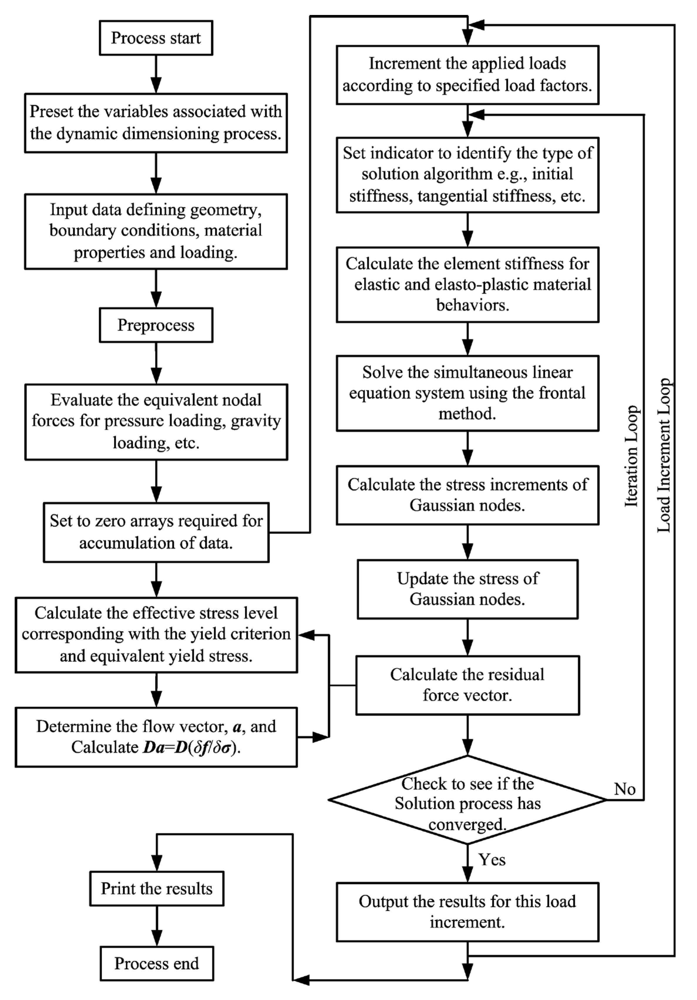
6. The Elasto-Plastic Cos-FEA Using MATLAB

Currently, numerous common methods like ABAQUS, FLAC or PLAXIS are applicable for the numerical analysis of layered rock masses. However, these methods are all developed on the basis of the classical continuum theory. What is more, they have not achieved the formulation of couple stress. As a result, they are unable to adequately interpret the bending deformation characteristics of layered rock masses. An efficient approach to addressing this issue is to write the Cos-FEA program by using MATLAB.

Based on the modified yield criteria, the elasto-plastic Cos-FEA programs were written by using MATLAB. And it was applied to the flexural deformation analysis of the two numerical examples that follow. The programming idea of Cos-FEA is consistent with the classical nonlinear FEA. The difference lies in the programming of the differential operator matrix L, the strain matrix B and the compliance matrix C. Additionally, as the Cosserat continuum theory features an extra rotational degree of freedom in contrast to the traditional continuum mechanics, this factor must be factored in during the formulation of the global stiffness matrix. In a manner similar to the programming thoughts of the classical nonlinear Finite Element Method, increments of the applied loads were configured in accordance with the given load factors, grounded on the theories of isotropic hardening and incremental plastic potential. Nonlinear equations were solved by using the Newton–Raphson method. During iterative loops, the residual force (that is, the difference between the equivalent node load and the external node load) is gradually reduced until the program reaches a state of convergence. Numerical procedures for conducting Cos-FEA can be found in Figure 4.

The convergence criterion of the FEA program is now based on the residual force values. The convergence criterion employed is similar to that described in Equation (33)

$${\displaystyle \frac{\sqrt{{\displaystyle \sum _{j=1}^N{({\psi }_j^i)}^2}}}{\sqrt{{\displaystyle \sum _{j=1}^N{(f_j)}^2}}}}\times 100\le \mathrm{TOLER}$$

(33)

where N is the total number of nodes, i denotes the iteration number, Ψ_jⁱ represents the j-th degree of freedom of the residual force at the i-th iteration, and f_j is the equivalent nodal force corresponding to the j-th degree of freedom. Equation (33) indicates that convergence is considered achieved if the difference in the norm of the residual forces between two successive iterations is less than or equal to TOLER times the norm of the total applied forces. In general, a value of TOLER ≤ 1.0% is deemed sufficient for most engineering applications.

7. Numerical Examples

The initial examples focus on cantilever layered plate structures featuring diverse geometries and boundary conditions, for which either an exact analytical solution or a close approximation exists. This example serves to validate the precision of the Cos-FEA method. The subsequent example examines the influence of out-of-plane layers on the three-dimensional deformation and stability analysis of an excavation within layered rock. In this scenario, the predictions made through the D-P criterion-based Cos-FEA are compared and validated against those generated using the traditional FEM.

7.1. Layered Cantilever Plate Subjected to a Transverse Shear Traction Force

The authors select a layered cantilever plate example for detailed derivation. Due to the length of the article, this section is not included in the paper.

As shown in Figure 5, the cantilever layered plate has a length of 15 m and a height of 1.5 m and is composed of three materials A, B and C; each layer has a thickness of 0.5 m and a 6.67 kPa transverse shear traction applied to the end of the plate. The Young’s modulus and Poisson’s ratio of each layer are chosen to be E_A = 10 × 10³ MPa, μ_A = 0.30, E_B = 15 × 10³ MPa, μ_B = 0.25, E_C = 20 × 10³ MPa and μ_C = 0.20. The normal stiffness is k_n = 1200 MPa/m, and the shear stiffness is k_s = 400 MPa/m for the layers of A, B and C.

The cantilever layered plate, which consists of three materials, is divided into 90 elements and 124 nodes. The mechanics of the materials, the classical continuum method, and the Cosserat medium method are used for the calculations, in which the mechanics of the materials is the analytical solution, and the last two are numerical solutions. By using these three methods to calculate the deflection of the tip of the cantilever layered plate, the accuracy of the Cosserat medium method is illustrated. The deflection of the tip of the cantilever layered plate predicted using the Cosserat solution is compared to the analytical solution by Timoshenko and Goodier [31]

$$u_3(l)={\displaystyle \frac{\tau bh{l}^3}{3{\displaystyle \sum _{i=1}^3{E}_i{I}_i}}}$$

(34)

As shown in

Table 2. The deflection of the tip of the cantilever layered plate.

Timoshenko Solution (mm)	Cosserat FEM of Solution (mm)	Traditional FEM of Solution (mm)
2.854	2.794	2.524

, the Cosserat medium method is more accurate than the classical continuum method and is closer to the analytical solution. This shows the feasibility of the Cosserat medium method and the correctness of the program. It also shows that under the action of load, the stress gradient is not negligible, the bending effect is obvious, and the Cosserat medium theory has better applicability and superiority.

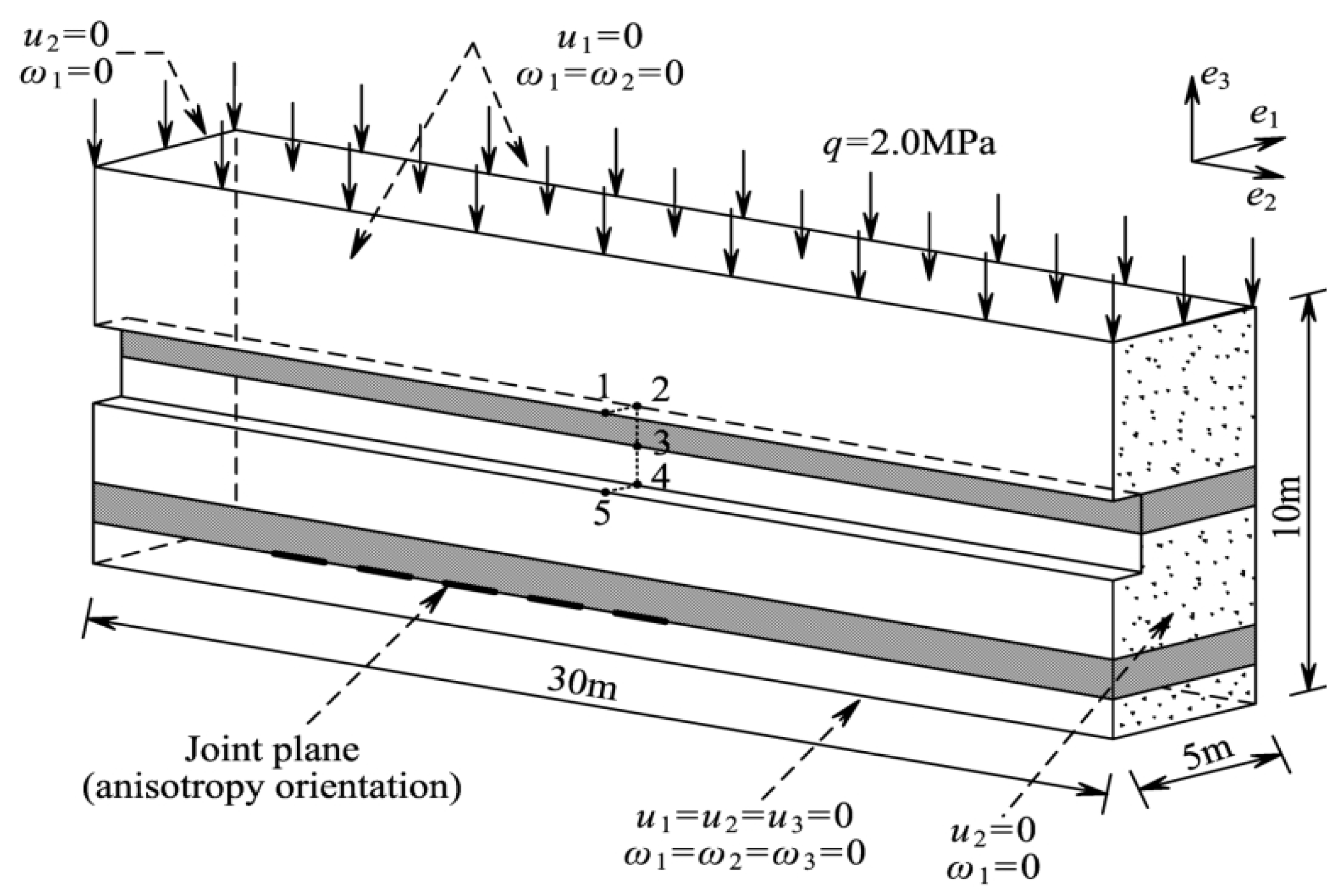
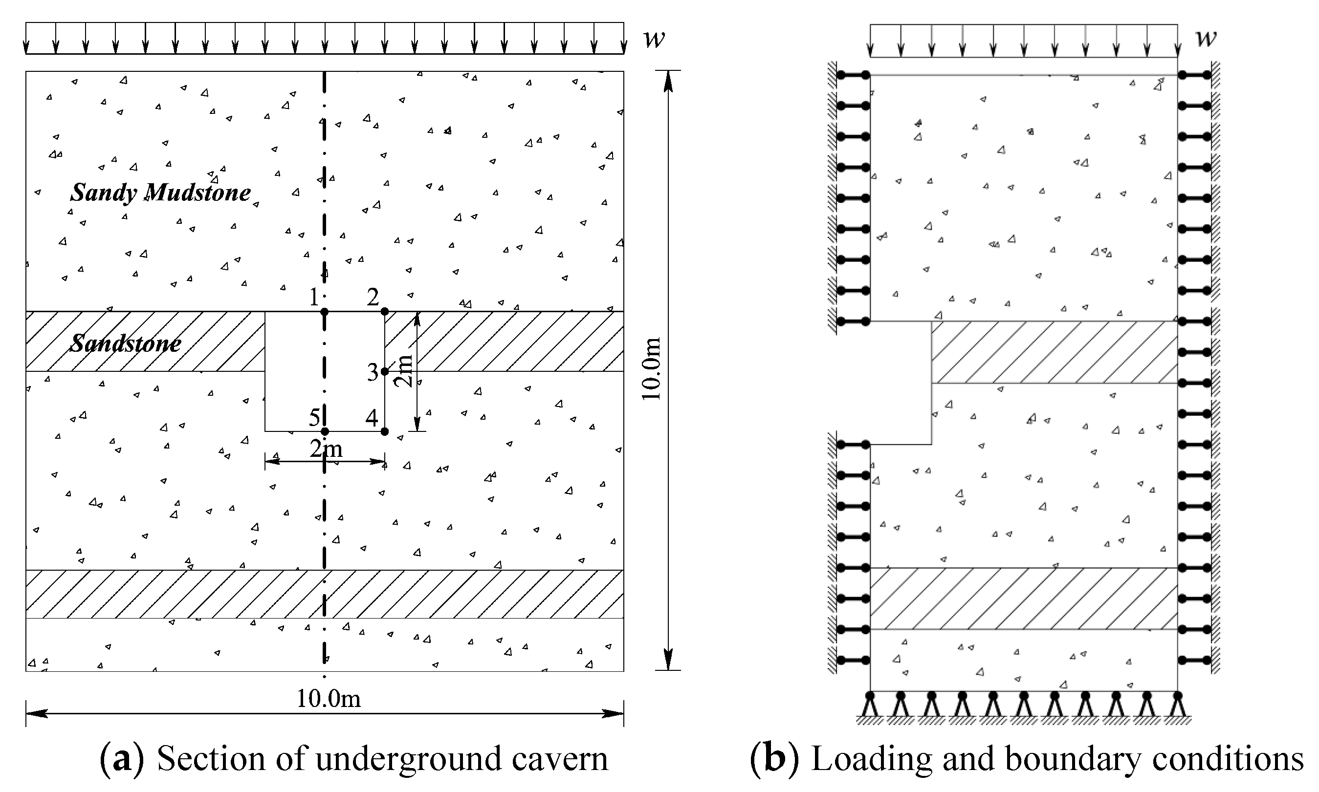
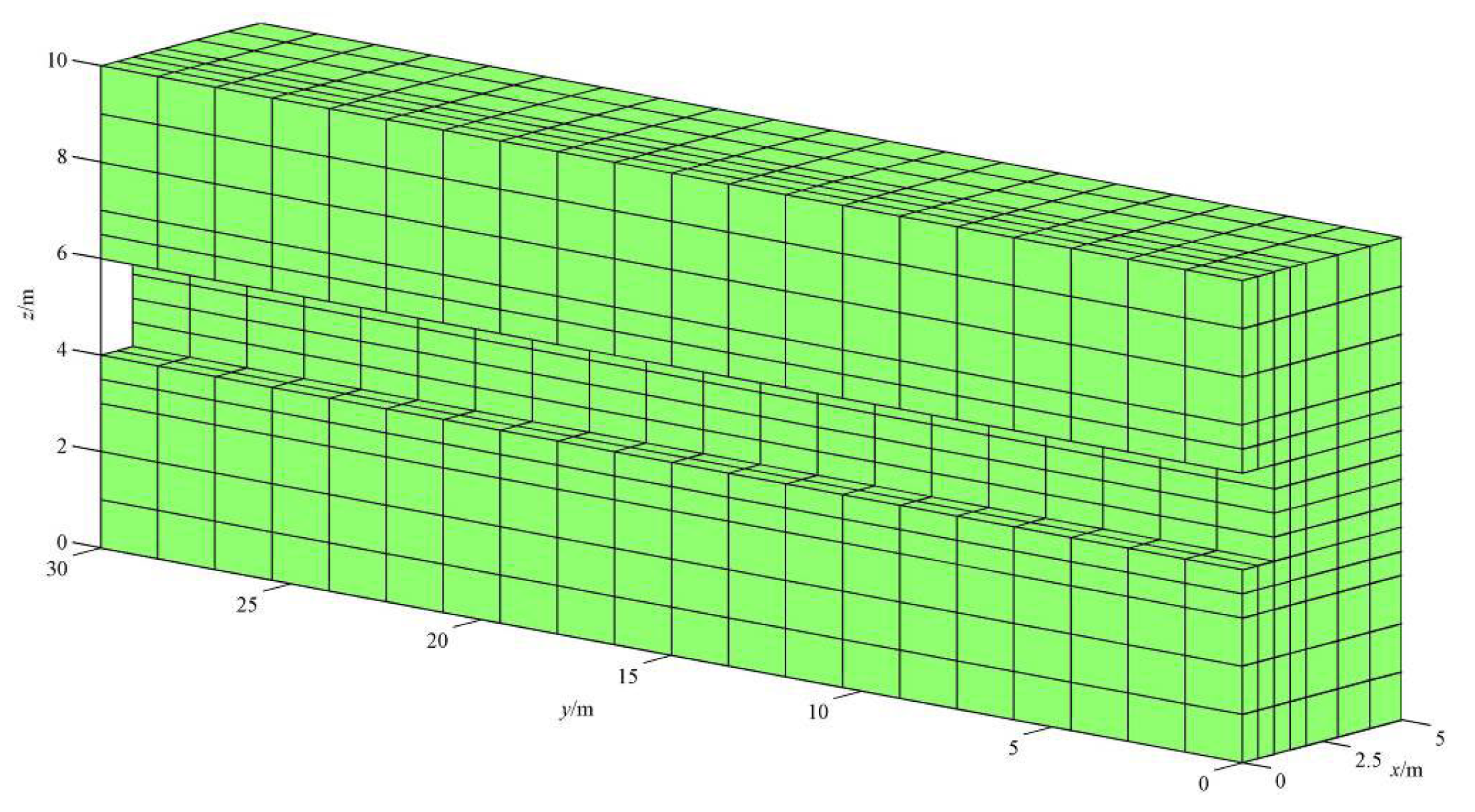
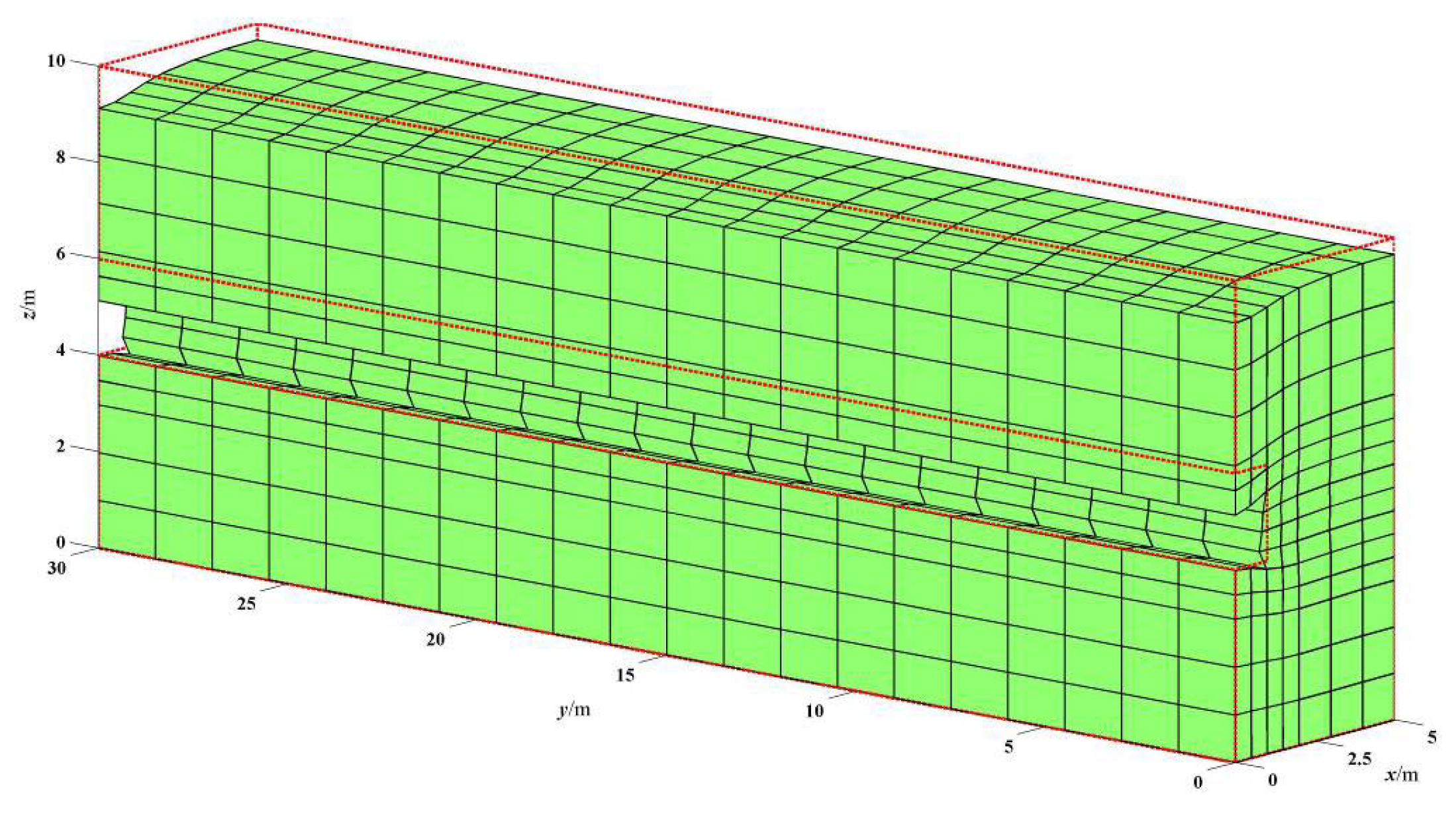
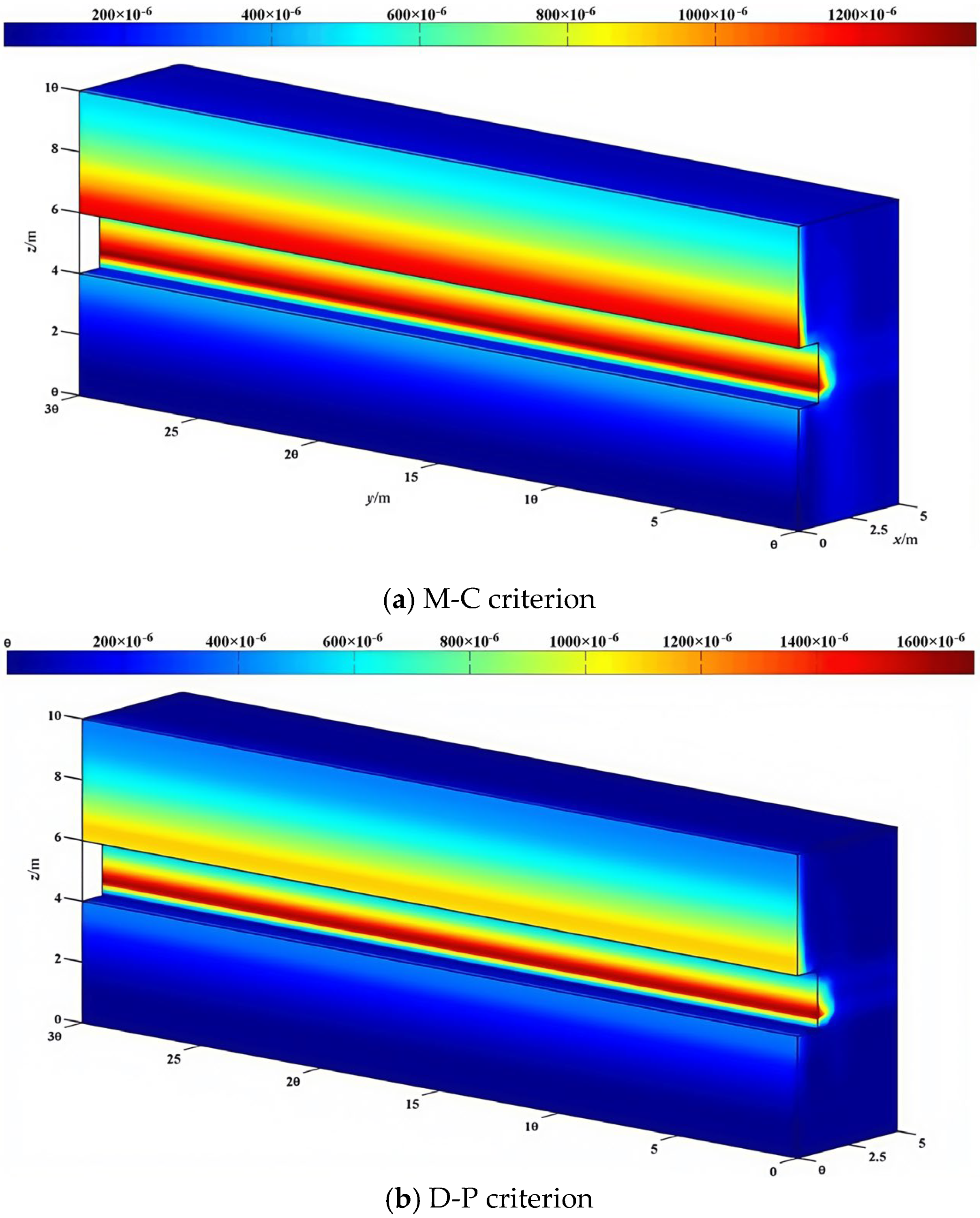
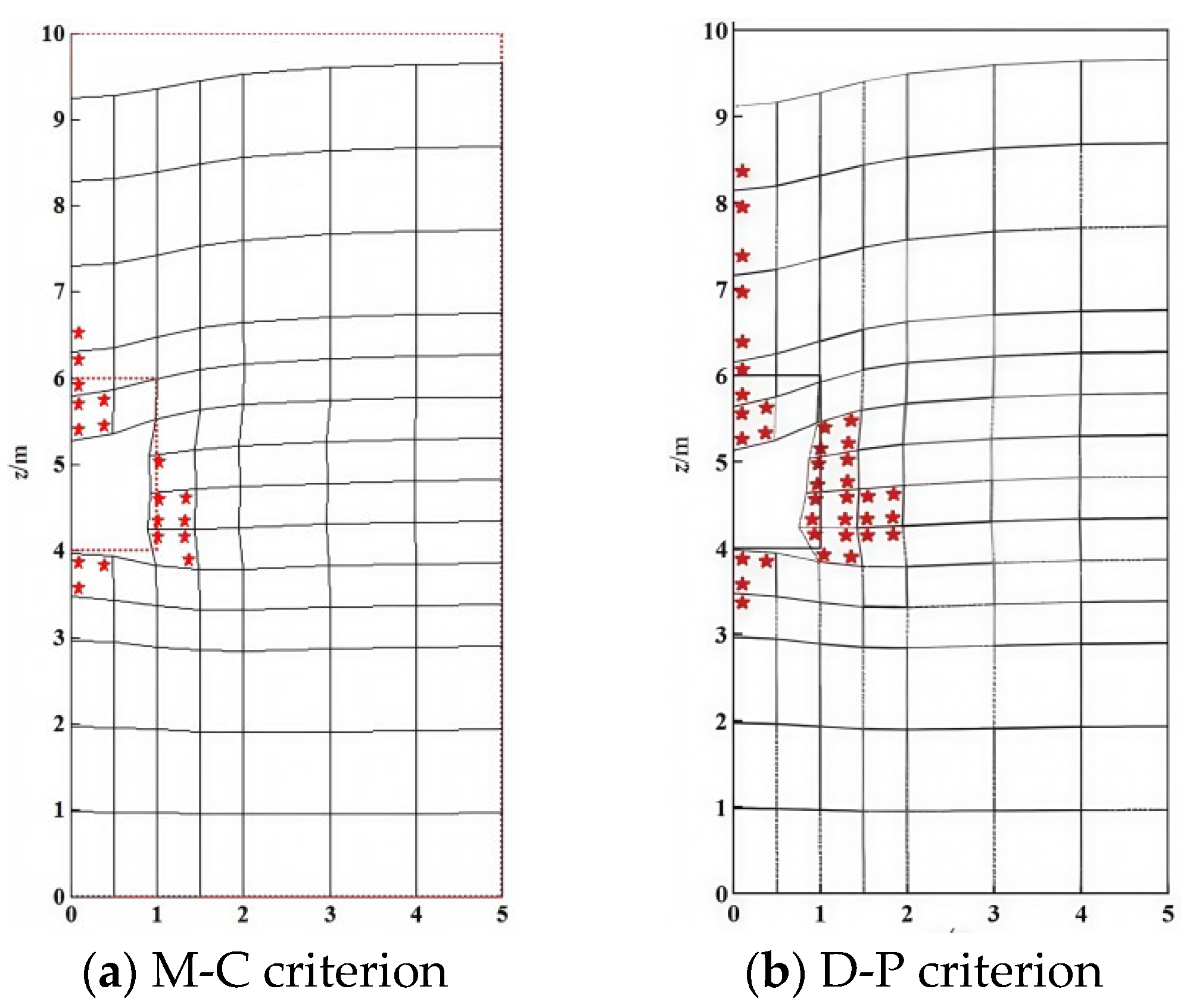
7.2. 3D Analysis of an Excavation in Layered Rock

This example investigates the impact of out-of-plane layers on the deformation and stability of an excavation. It highlights the effectiveness and precision of the Cos-FEA method in predicting the behavior of layered structures. Figure 6 illustrates the geometry, boundary conditions, loading configuration and definition of layer orientation for this problem. Due to the symmetry of the problem, we study only a quarter of it, as shown in Figure 7. The basic parameters of the interstratified rock mass are listed in

Table 3. Basic parameters of the layered rock mass.

	Name	Sandstone	Sandy Mudstone
Parameters
Volume concentration (n)/%		25.0	75.0
Volume density (k)/kN·m−3		24.9	25.8
Elastic modulus (E)/GPa		21.78	5.15
Internal friction angle (γ)/°		26.0	34.0
Cohesive strength (σc)/MPa		1.40	0.75
Poisson’s ratio (μ)		0.23	0.31

. The length of the chamber is set to 30 m, and a uniform pressure of 2.0 MPa is applied to the top surface. Using its symmetry, half of the model is simulated with 1800 eight-node equal-parameter brick elements.

Element type: eight-node brick element;

Number of elements: 1800;

Number of elements in out-of-plane direction: 20;

Number of FEM nodes: 2394;

Number of degrees of freedom in 3D space: 11,357.

The Cosserat FEM (CFEM) mesh discretization of the structure is shown in Figure 8. The numerical deformed configuration diagram is exhibited in Figure 9. Moreover, the contour maps of vertical displacement, the maximum principal stress and the maximum shear strain at failure were obtained by using the M-C criterion-based CFEM (CFEM M-C) and the D-P criterion-based CFEM (CFEM D-P), as shown in Figure 10, Figure 11, Figure 12 and Figure 13. The mesh grid of structural deformation is enlarged by 200 times, where red stars represent the yielded Gaussian points, as shown in Figure 13. As can be seen from Figure 10, Figure 11, Figure 12 and Figure 13, the results calculated by the D-P criterion are larger, and the damage area of the cavern is predicted to be wider. Due to the stress concentration, the maximum compressive stress occurs in the area of abrupt shape, that is, the four corners of the cavern. The maximum tensile stress is concentrated on the side wall, top and bottom of the cavern, which is consistent with the location of the failure phenomena, such as rock bending, that occur when the cavern is excavated in the layered rock mass. In addition, due to the equivalence of the Cosserat extended model, the contour maps calculated using the two intensity criteria appear to be relatively smooth. The load factors are accessed on the first iteration of each load increment. In this program, they were specified as 0.8 and 0.2, so the total load acting on the structure during the second increment is 1.0 times the calculated loads. Figure 14 indicates that when computation convergence is attained, the M-C criterion-based Cosserat FEM (CFEM M-C) need to finish 102 iterations, and the D-P criterion-based Cosserat FEM (CFEM D-P) only needs 18 iterations. The former was approximately six times more than the latter.

Displacements of all tracking points at the middle section (z = 15 m) by the CFEM M-C and CFEM D-P are listed in

Table 4. Displacements of all tracking points at the middle section (z = 15 m) using Cosserat FEM analysis, with anisotropy orientation.

Tracking Points (Coordinate)	D-P			M-C
	u1/mm	u3/mm	ω2/mrad	u1/mm	u3/mm	ω2/mrad
1 (0, 15, 6)	0.000	−4.350	0.000	0.000	−3.619	0.000
2 (1, 15, 6)	−0.174	−2.740	−1.806	−0.090	−2.361	−1.485
3 (1, 15, 5)	−0.822	−1.820	−0.462	−0.360	−1.609	−0.370
4 (1, 15, 4)	−0.105	−0.790	0.829	−0.101	−0.814	0.810
5 (0, 15, 4)	0.000	−0.080	0.000	0.000	−0.120	0.000

Unwritten displacements u₂, ω₁ and ω₃ are zero.

. As shown in Table 4, the following information can be obtained: With the release of stratigraphic stress, because of the symmetry of structure and loading, the horizontal displacements of points 1 and 5 are zero. And that vertical displacement of point 1 is the highest. As can be seen from Figure 15, based on the M-C and D-P criteria, u₃ of each tracking point are calculated by using four methods: Cosserat Finite Element Method (CFEM) and Traditional Finite Element Method (TFEM), respectively. Figure 15 also indicate that the analytical results are close, especially at the tracking points 3, 4 and 5. Meanwhile, the small plot in Figure 15 represents the variance of u₃ calculated using the four methods at each tracking point. The max value of variance is only 0.6554 mm². It shows that on the basis of the above two criteria, the four methods were reliable. However, for the positions of the structure with an obvious stress gradient or bending effect, i.e., the top of cave point 1 and the corner of cave point 2, the results of the M-C- and D-P-based Cosserat medium methods are larger. Moreover, the D-P-based Cos-FEA is approximately twice the M-C-based Cos-FEA.

8. Conclusions

In order to account for some major stratigraphic characteristics of the layered rocks, i.e., features that have a major influence on the mechanical behavior of excavations in these deposits, the application of two modified strength criteria to a Cosserat-like medium constitutive model for bedded rocks is proposed. The major conclusions are summarized as follows:

(1)

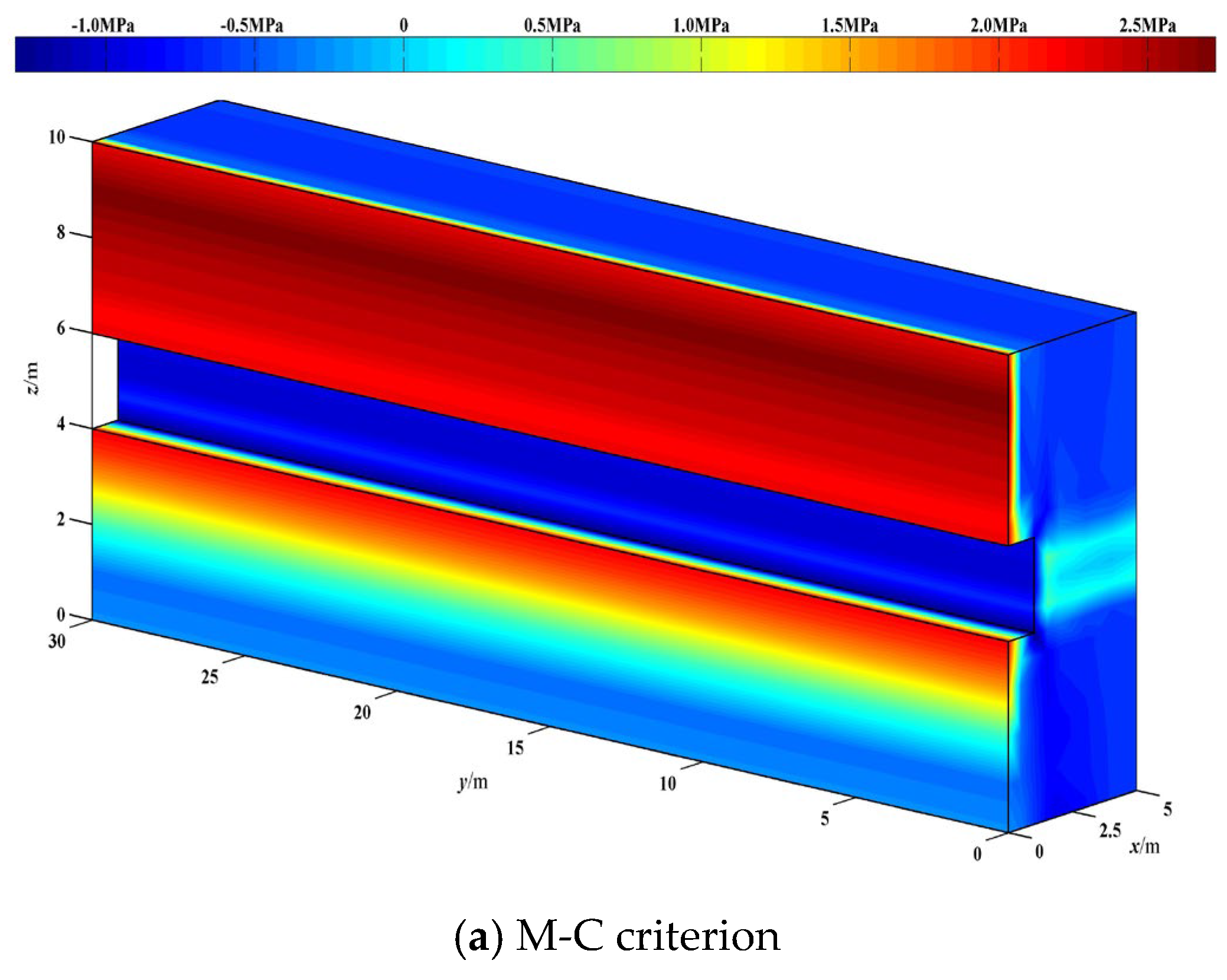
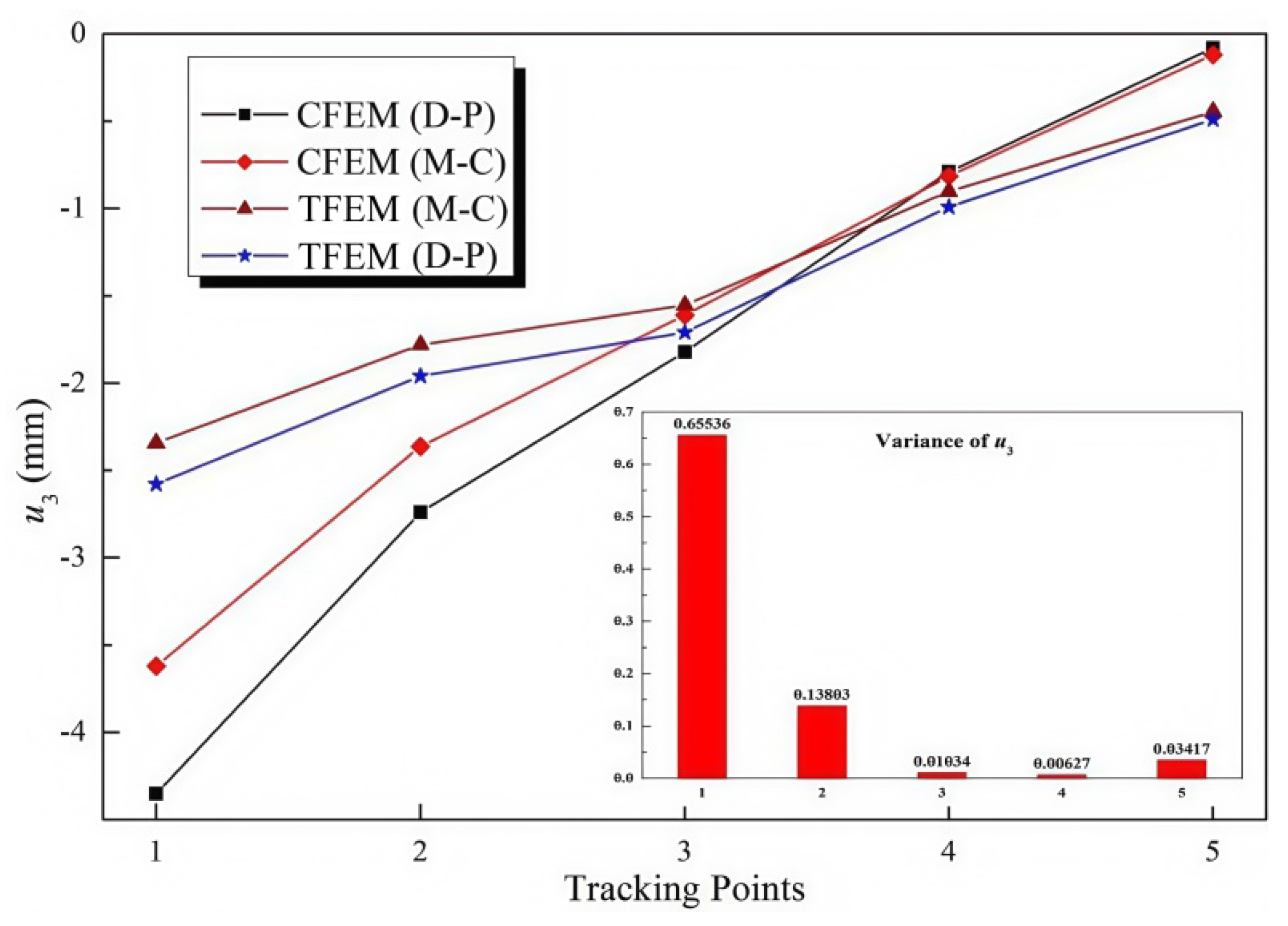
The numerical simulation examples showed that based on M-C and D-P criteria, the Cos-FEA was effective in analyzing the flexural deformation of an underground cave in an alternating rock mass. The vertical displacement (u₃) value of the top cavern calculated using the D-P criterion was found to be higher than that of the modified M-C method. However, horizontal displacements of the former were lower than the latter.

(2)

Under the same calculation capacity, the D-P criterion-based Cos-FEA was observed to have a higher convergence speed and a lower number of iterations when compared with that based on the M-C criterion.

(3)

Since the M-C hexagonal yield surface is not smooth but has corners, these corners of the hexagon can cause numerical difficulty in its application to the asymmetric Cosserat constitutive relationship. However, the D-P criterion can be viewed as a smooth approximation of the M-C criterion to avoid such difficulty, and the D-P criterion can be made to match the M-C criterion by adjusting the size of the cone. Meanwhile, the M-C criterion does not take into account the influence of the intermediate principal stress on strength, but the D-P criterion is able to reflect the combined effect of the three principal stresses. Thus, the D-P criterion-based Cos-FEA is observed to have a higher convergence speed and stability.

It should be noted that the present numerical model is based on a simplified version of the proposed Cosserat expanded constitutive theory for taking into account the influence of bending and needs further development, especially for creep damage, as well as the influence of possible healing.

References

1. Cosserat, E.; Cosserat, F. Théorie des Corps Déformables; A. Herman et Fils: Paris, France, 1909. [Google Scholar]
2. Marin, M.; Seadawy, A.; Vlase, S.; Chirila, A. On mixed problem in thermoelasticity of type III for Cosserat media. J. Taibah Univ. Sci. 2022, 16, 1264–1274. [Google Scholar] [CrossRef]
3. Alavi, S.; Ganghoffer, J.; Sadighi, M.; Nasimsobhan, M.; Akbarzadeh, A. Continualization method of lattice materials and analysis of size effects revisited based on Cosserat models. Int. J. Solids Struct. 2022, 254, 111894. [Google Scholar] [CrossRef]
4. Surówka, P.; Souslov, A.; Jülicher, F.; Banerjee, D. Odd Cosserat elasticity in active materials. Phys. Rev. E 2023, 108, 064609. [Google Scholar] [PubMed]
5. Tummers, M.; Lebastard, V.; Boyer, F.; Troccaz, J.; Rosa, B.; Chikhaoui, M.T. Cosserat rod modeling of continuum robots from newtonian and lagrangian perspectives. IEEE Trans. Robot. 2023, 39, 2360–2378. [Google Scholar]
6. Marin, M.; Carrera, E.; Othman, M.I.A.; Abbas, I. A variational approach of the boundary value problem for elastic Cosserat bodies. Mech. Adv. Mater. Struct. 2024, 31, 58–63. [Google Scholar]
7. Ghiba, I.-D.; Rizzi, G.; Madeo, A.; Neff, P. Cosserat micropolar elasticity: Classical Eringen vs. dislocation form. J. Mech. Mater. Struct. 2023, 18, 93–123. [Google Scholar]
8. Song, X.; Pashazad, H. Computational Cosserat periporomechanics for strain localization and cracking in deformable porous media. Int. J. Solids Struct. 2024, 288, 112593. [Google Scholar] [CrossRef]
9. Adhikary, D.P.; Mühlhaus, H.B.; Dyskin, A.V. A numerical study of flexural buckling of foliated rock slopes. Int. J. Numer. Anal. Methods Geomech. 2001, 30, 871–884. [Google Scholar]
10. Mühlhaus, H. Continuum models for layered and blocky rock. Compr. Rock Eng. 2014, 2, 209–231. [Google Scholar]
11. She, C.; Xiong, W.; Chen, S. Elasto-visco plastic Cosserat theory of layered rock mass and its application in engineering. J. Hydraul. Eng. 1996, 4, 10–17. [Google Scholar]
12. Li, Y.P.; Yang, C.H. Three-dimensional expanded Cosserat medium constitutive model for laminated salt rock. Rock Soil Mech. 2006, 27, 509–513. [Google Scholar]
13. Marin, M.; Fudulu, I.M.; Vlase, S. On some qualitative results in thermodynamics of Cosserat bodies. Bound. Value Probl. 2022, 2022, 69. [Google Scholar]
14. Li, H.; Xun, L.; Zheng, G.; Renda, F. Discrete cosserat static model-based control of soft manipulator. IEEE Robot. Autom. Lett. 2023, 8, 1739–1746. [Google Scholar]
15. Nebel, L.J.; Sander, O.; Bîrsan, M.; Neff, P. A geometrically nonlinear Cosserat shell model for orientable and non-orientable surfaces: Discretization with geometric finite elements. Comput. Methods Appl. Mech. Eng. 2023, 416, 116309. [Google Scholar]
16. Yu, F.; Huang, G.; Li, W.; Ni, H.; Huang, B.; Li, J.; Duan, J. Modeling lateral vibration of bottom hole assembly using Cosserat theory and laboratory experiment verification. Geoenergy Sci. Eng. 2023, 222, 211359. [Google Scholar]
17. Boyer, F.; Lebastard, V.; Candelier, F.; Renda, F.; Alamir, M. Statics and dynamics of continuum robots based on Cosserat rods and optimal control theories. IEEE Trans. Robot. 2022, 39, 1544–1562. [Google Scholar]
18. Tuan, L.T.; Dung, N.T.; Van Thom, D.; Van Minh, P.; Zenkour, A.M. Propagation of non-stationary kinematic disturbances from a spherical cavity in the pseudo-elastic cosserat medium. Eur. Phys. J. Plus 2021, 136, 1–16. [Google Scholar]
19. Tang, H.; Wei, W.; Liu, F.; Chen, G. Elastoplastic Cosserat continuum model considering strength anisotropy and its application to the analysis of slope stability. Comput. Geotech. 2020, 117, 103235. [Google Scholar]
20. Tang, H.; Wei, W.; Song, X.; Liu, F. An anisotropic elastoplastic Cosserat continuum model for shear failure in stratified geomaterials. Eng. Geol. 2021, 293, 106304. [Google Scholar]
21. Reda, H.; Alavi, S.; Nasimsobhan, M.; Ganghoffer, J. Homogenization towards chiral Cosserat continua and applications to enhanced Timoshenko beam theories. Mech. Mater. 2021, 155, 103728. [Google Scholar]
22. Armanini, C.; Hussain, I.; Iqbal, M.Z.; Gan, D.; Prattichizzo, D.; Renda, F. Discrete cosserat approach for closed-chain soft robots: Application to the fin-ray finger. IEEE Trans. Robot. 2021, 37, 2083–2098. [Google Scholar] [CrossRef]
23. Ghiba, I.D.; Bîrsan, M.; Lewintan, P.; Neff, P. The isotropic Cosserat shell model including terms up to O (h 5). Part I: Derivation in matrix notation. J. Elast. 2020, 142, 201–262. [Google Scholar] [CrossRef]
24. Colatosti, M.; Fantuzzi, N.; Trovalusci, P.; Masiani, R. New insights on homogenization for hexagonal-shaped composites as Cosserat continua. Meccanica 2022, 57, 885–904. [Google Scholar] [CrossRef]
25. Shirani, M.; Steigmann, D.J. A Cosserat model of elastic solids reinforced by a family of curved and twisted fibers. Symmetry 2020, 12, 1133. [Google Scholar] [CrossRef]
26. Giorgio, I.; De Angelo, M.; Turco, E.; Misra, A. A Biot–Cosserat two-dimensional elastic nonlinear model for a micromorphic medium. Contin. Mech. Thermodyn. 2020, 32, 1357–1369. [Google Scholar] [CrossRef]
27. Chen, K.; Zou, D.; Tang, H.; Liu, J.; Zhuo, Y. Scaled boundary polygon formula for Cosserat continuum and its verification. Eng. Anal. Bound. Elem. 2021, 126, 136–150. [Google Scholar] [CrossRef]
28. Fantuzzi, N.; Trovalusci, P.; Luciano, R. Material symmetries in homogenized hexagonal-shaped composites as Cosserat continua. Symmetry 2020, 12, 441. [Google Scholar] [CrossRef]
29. Russo, R.; Forest, S.; Girot Mata, F.A. Thermomechanics of Cosserat medium: Modeling adiabatic shear bands in metals. Contin. Mech. Thermodyn. 2020, 35, 919–938. [Google Scholar] [CrossRef]
30. Orekhov, A.L.; Simaan, N. Solving cosserat rod models via collocation and the magnus expansion. In Proceedings of the 2020 IEEE/RSJ International Conference on Intelligent Robots and Systems (IROS), Las Vegas, NV, USA, 24 October 2020–24 January 2021; pp. 8653–8660. [Google Scholar]
31. Timoshenko, S.; Goodier, J.N. Theory of Elasticity, 3rd ed.; McGraw-Hill: New York, NY, USA, 1970. [Google Scholar]
Figure 1. Schematic of the stress components of the three-dimensional Cosserat continuum on the alternating layered rock mass.
Applsci 15 03604 g001
Figure 2. A 3D representation of stress and couple stress measures.
Applsci 15 03604 g002
Figure 3. M-C and D-P criteria when they coincide along the compressive meridian.
Applsci 15 03604 g003
Figure 4. Numerical procedures for Cosserat FEM calculations.
Applsci 15 03604 g004
Figure 5. Geometry, boundary conditions, loading and mesh for a cantilever layered plate.
Applsci 15 03604 g005
Figure 6. The geometric dimensions, boundary conditions and loads of the model.
Applsci 15 03604 g006
Figure 7. Calculating schematic of a square tunnel in an interlayered rock mass.
Applsci 15 03604 g007
Figure 8. Cos-FEA mesh discretization of structure.
Applsci 15 03604 g008
Figure 9. Numerical deformed configuration diagram. The red frame represents the dimensions of the structure that are not deformed.
Applsci 15 03604 g009
Figure 10. Contour map of vertical displacement (u3) using D-P method.
Applsci 15 03604 g010
Figure 11. Contour maps of the maximum principal stress at failure.
Applsci 15 03604 g011aApplsci 15 03604 g011b
Figure 12. Contour maps of the maximum shear strain at failure.
Applsci 15 03604 g012
Figure 13. Distribution diagram of plastic zones.
Applsci 15 03604 g013
Figure 14. The effect of convergence by two criteria.
Applsci 15 03604 g014
Figure 15. Vertical displacements (u3) of all tracking points using Cosserat FEM and traditional FEM.
Applsci 15 03604 g015