Three-Dimensional Geological Modeling Method Based on Potential Vector Fields

Abstract

With the development of 3D geological modeling, implicit modeling methods have gradually gained popularity. However, existing potential field methods cannot directly represent unconformable geological interfaces. In response, an implicit modeling method based on a potential vector field was proposed, which generates geological surface models through the potential vector field method and generalized marching cubes algorithm, and visualizes the modeling results. An experiment was conducted on the study area of a certain mineral deposit, and a 3D geological surface model with consistency and no topological errors was established, demonstrating the effectiveness of the method for the surface modeling of unconformity geological interfaces.

1. Introduction

Three-dimensional geological modeling uses mathematical methods to construct the geometric models of geological bodies according to geological rules (surface model) or the spatial distribution of physical property indicators (voxel model) [1,2]. This technique plays a significant role in geological research. Wang et al. [3] implemented 3D geological modeling in urban underground space planning for Shenyang City, ensuring spatial coordination across multiple dimensions. Guo et al. [4] developed integrated 3D geological models for volcanic systems, achieving geometric fusion of diverse complex geological structures. Yang et al. [5] established a comprehensive 3D geological modeling framework utilizing geospatial data from Singapore, accompanied by the development of a specialized model management system. The methodology demonstrates exceptional capability in providing flexible and intuitive representation of geological structures, stratigraphy, lithology, and other geological conditions [6,7].

The 3D geological surface modeling methods primarily include explicit modeling and implicit modeling. The explicit modeling method defines each object in the model explicitly, directly obtaining the coordinates of points, lines, and faces of the geological objects to form surfaces [4], such as the cross-section method [8], Coons surfaces [9], Bézier curve/surfaces [10], etc. However, it has certain limitations: (1) it requires significant manual interaction and is inefficient for modeling complex shapes; (2) the results often contains topological errors, such as triangle intersections, which require subsequent verification and correction; and (3) different modelers may have varying skills and understandings, which can lead to uncertainty and multiple solutions in the model [11,12]. The implicit modeling method treats the entire stratigraphic space as a potential field, which is a scalar field defined by an implicit function. The geological interfaces are defined as isosurfaces in the potential field [13]. In implicit modeling, the implicit function is first selected, and the unknowns quantities in the function are solved using known constraints, thereby establishing the potential field. The 3D geological surface model is then obtained using surface generation algorithms. Compared with explicit modeling, implicit modeling has advantages such as faster modeling speed, no need for manual interactions, and real-time dynamic modeling [14,15,16].

The key to establishing a potential field lies in the interpolation method [17]. Commonly used methods include Kriging interpolation [18,19,20,21], radial basis function (RBF) interpolation [3,16,22,23,24,25], etc. Kriging interpolation requires the data to follow a normal distribution, and it is difficult for data with large variations in spatial density to meet this requirement. In contrast, RBF interpolation has lower data requirements and performs better when constructing complex surfaces [26].

Surface generation algorithms divide the entire space into basic voxel units and compute the potential field values at the vertices of these voxel units using the implicit function. Within each voxel unit, triangular facets are used to approximate the isosurface. Depending on the type of basic voxel unit, the algorithms can be divided into marching cubes (MCs) [27] and marching tetrahedra (MTs) [28]. Compared to the MT algorithm, the MC algorithm is more complex but does not require additional tracking of the grid’s topological information. Additionally, when the number of voxel units is roughly the same, the MC algorithm offers higher approximation accuracy [29].

The potential field function is continuous throughout the space and cannot represent unconformable stratigraphic interfaces, such as pinch-outs and erosions. Many researchers have chosen to post-process modeling results to extract unconformable stratigraphic interfaces [26], but this compromises the consistency of the model and consequently affects its quality. Furthermore, current MC algorithms can only handle interface between two regions and cannot address multi-region interfaces at unconformable stratigraphic interfaces. A potential vector field method is proposed to solve the issue of representing unconformable stratigraphic interfaces using potential field functions. A generalized marching cubes algorithm is introduced to handle the surface generation of multi-region interfaces. An experiment was conducted on a mining study area with unconformable stratigraphic interfaces, and a consistent 3D geological surface model without topological errors was established. The results demonstrate the effectiveness of the proposed method for modeling unconformable stratigraphic interfaces.

2. Materials and Methods

In this section, the potential vector field method and the generalized marching cubes algorithm are first introduced. Then, the entire modeling process is presented in conjunction with actual borehole data.

2.1. Potential Vector Field Method

In the potential field method, the potential field is a scalar function $f:{\mathbb{R}}^3\to \mathbb{R}$ defined in space, where the independent variable $\mathit{x}=(x, y, z)\in {\mathbb{R}}^3$ represents spatial coordinates. Due to the gradual variation of the potential field values within each stratum, countless non-intersecting equipotential surfaces exist. Each geological interface has a specific potential field value, allowing the interface to be represented as a series of specific isosurfaces $f\left(\mathit{x}\right)=s_k$ (where $k=1, \dots , K$). Different interfaces correspond to different potential field values; therefore, this definition is unable to represent multi-region interfaces at unconformable stratigraphic interfaces.

In response, we propose the potential vector field function representation. Suppose there are l strata in the study area, and a vector function $\mathit{f}\left(\mathit{x}\right)=(f_1\left(\mathit{x}\right), f_2\left(\mathit{x}\right), \dots , f_l\left(\mathit{x}\right))\in {\mathbb{R}}^3$ is defined in the space. For any point ${\mathit{x}}_0$ in the space, the t-th component of the function, $f_t\left(\mathit{x}\right)$, can be determined as follows: Let the distances from the point ${\mathit{x}}_0$ to the upper and lower interfaces of stratum t in the vertical direction be $d_1$ and $d_2$, respectively. Then, according to

$$f_t\left({\mathit{x}}_0\right)=\left\{\begin{array}{cc}\min \left\{d_1, d_2\right\}\hfill & \left({\mathit{x}}_0\mathrm{is}\mathrm{inside}\mathrm{stratum}t\right)\hfill \\ -\min \{d_1, d_2\}\hfill & \left({\mathit{x}}_0\mathrm{is}\mathrm{outside}\mathrm{stratum}t\right)\hfill \\ 0\hfill & \left({\mathit{x}}_0\mathrm{is}\mathrm{at}\mathrm{the}\mathrm{interface}\mathrm{of}\mathrm{stratum}t\right)\hfill \end{array}\right.,$$

(1)

it is evident that $f_t\left({\mathit{x}}_0\right)$ represents the distance in the vertical direction from point ${\mathit{x}}_0$ to the closer of the two interfaces (upper or lower) of stratum t, with its sign indicating the relative position to stratum t. A positive value indicates that the point is inside the stratum, while a negative value indicates it is outside the stratum. Specifically, when point ${\mathit{x}}_0$ lies exactly on the interface of stratum t, $f_t\left({\mathit{x}}_0\right)=0$.

When point ${\mathit{x}}_0$ is inside or on the interface of stratum k, it is evident that

$$f_t\left({\mathit{x}}_0\right)=\left\{\begin{array}{cc}{f}_t\left({\mathit{x}}_0\right)\ge 0\hfill & (t=k)\hfill \\ f_t\left({\mathit{x}}_0\right)<0\hfill & (t\ne k)\hfill \end{array}\right.,$$

(2)

However, due to potential computational errors, Equation (2) is not suitable for direct solution. Nevertheless, it can be observed that, under ideal conditions, the k-th component of $\mathit{f}\left(\mathit{x}\right)$ is always non-negative within stratum k, while all other components remain negative. Based on this observation, stratum k can be represented as

$$f_k\left(\mathit{x}\right)=\max \left\{f_1\left(\mathit{x}\right), f_2\left(\mathit{x}\right), \dots , f_l\left(\mathit{x}\right)\right\}$$

(3)

That is, for any point $\mathit{x}$ within stratum k, the k-th component of $\mathit{f}\left(\mathit{x}\right)$ is always the largest component.

Similarly, the interface between strata $k_1$ and $k_2$ can be represented as

$$f_{k_1}\left(\mathit{x}\right)=f_{k_2}\left(\mathit{x}\right)=\max \left\{f_1\left(\mathit{x}\right), f_2\left(\mathit{x}\right), \dots , f_l\left(\mathit{x}\right)\right\}.$$

(4)

The intersection of strata $k_1$, $k_2$ and $k_3$ can be represented as

$$f_{k_1}\left(\mathit{x}\right)=f_{k_2}\left(\mathit{x}\right)=f_{k_3}\left(\mathit{x}\right)=\max \left\{f_1\left(\mathit{x}\right), f_2\left(\mathit{x}\right), \dots , f_l\left(\mathit{x}\right)\right\}$$

(5)

Given a set of data points ${\{{\mathit{x}}_i, {\mathit{s}}_i\}}_{i=1}^n\in {\mathbb{R}}^3\times {\mathbb{R}}^l$, where ${\mathit{x}}_i$ is the spatial coordinates of i-th point and ${\mathit{s}}_i=(s_{i1}, s_{i2}, \dots , s_{il})$ is the potential vector field value at i-th point, the potential vector field function is obtained through radial basis function interpolation. The goal is to find an interpolation function of the following form:

$$\mathit{f}\left(\mathit{x}\right)=\sum _{j=1}^n{\mathit{\lambda }}_j\phi \left(\parallel \mathit{x}-{\mathit{x}}_j\parallel \right)+\mathit{p}\left(\mathit{x}\right),$$

(6)

where ${\mathit{\lambda }}_j=({\mathbf{\lambda }}_{j1}, {\mathbf{\lambda }}_{j2}, \dots , {\mathbf{\lambda }}_{jl})$ ($j=1, \dots , n$) is the undetermined coefficient, $\parallel \mathit{x}-{\mathit{x}}_j\parallel$ denotes the Euclidean distance between the points $\mathit{x}$ and ${\mathit{x}}_j$, $\phi \left(\left(\parallel \mathit{x}-{\mathit{x}}_j\parallel \right)\right)=\sqrt{{\left(\parallel \mathit{x}-{\mathit{x}}_j\parallel \right)}^2+c^2}$ is the radial basis function, and c is the shape parameter of the function. The polynomial terms are given by $\mathit{p}\left(\mathit{x}\right)={\mathit{a}}_1+{\mathit{a}}_{2}x+{\mathit{a}}_{3}y+{\mathit{a}}_{4}z$, and ${\mathit{a}}_j=(a_{j1}, a_{j2}, \dots , a_{jl})$ ($j=1, 2, 3, 4$) are the undetermined coefficients.

The interpolation function satisfies the constraints $\mathit{f}\left({\mathit{x}}_i\right)={\mathit{s}}_i$ ($i=1, \dots , n$), which provide n equations, while the number of unknown coefficients is $(n+4)l$. Since the number of equations is insufficient, orthogonality constraints are needed:

$$\underset{j=1}{\sum ^n}{\mathit{\lambda }}_j=\underset{j=1}{\sum ^n}{\mathit{\lambda }}_j{x}_j=\underset{j=1}{\sum ^n}{\mathit{\lambda }}_j{y}_j=\underset{j=1}{\sum ^n}{\mathit{\lambda }}_j{z}_j=\mathbf{0}$$

(7)

where the final system of equations is given by

$$\left\{\begin{array}{cc}\hfill & {\displaystyle \underset{j=1}{\sum ^n}}{\mathit{\lambda }}_j\phi \left(\parallel {\mathit{x}}_i-{\mathit{x}}_j\parallel \right)+\mathit{p}\left({\mathit{x}}_i\right)(i=1, \dots , n)\hfill \\ \hfill & {\displaystyle \underset{j=1}{\sum ^n}}{\mathit{\lambda }}_j={\displaystyle \underset{j=1}{\sum ^n}}{\mathit{\lambda }}_j{x}_j={\displaystyle \underset{j=1}{\sum ^n}}{\mathit{\lambda }}_j{y}_j={\displaystyle \underset{j=1}{\sum ^n}}{\mathit{\lambda }}_j{z}_j=\mathbf{0}\hfill \end{array}\right.$$

(8)

Let ${\phi }_{ij}=\phi \left(\parallel {\mathit{x}}_i-{\mathit{x}}_j\parallel \right)$, $\mathsf{\Phi }=\left[\begin{array}{cccc}{\phi }_{11}& {\phi }_{12}& \dots & {\phi }_{1n}\\ {\phi }_{21}& {\phi }_{22}& \dots & {\phi }_{2n}\\ ⋮& ⋮& \ddots & ⋮\\ {\phi }_{n1}& {\phi }_{n2}& \dots & {\phi }_{nn}\end{array}\right]$, $\mathsf{\Lambda }=\left[\begin{array}{cccc}{\lambda }_{11}& {\lambda }_{12}& \dots & {\lambda }_{1l}\\ {\lambda }_{21}& {\lambda }_{22}& \dots & {\lambda }_{2l}\\ ⋮& ⋮& \ddots & ⋮\\ {\lambda }_{n1}& {\lambda }_{n2}& \dots & {\lambda }_{nl}\end{array}\right]$, $\mathit{S}=\left[\begin{array}{cccc}{s}_{11}& s_{12}& \dots & s_{1l}\\ s_{21}& s_{22}& \dots & s_{2l}\\ ⋮& ⋮& \ddots & ⋮\\ s_{n1}& s_{n2}& \dots & s_{nl}\end{array}\right]$, $\mathit{P}=\left[\begin{array}{cccc}1& x_1& y_1& z_1\\ 1& x_2& y_2& z_2\\ ⋮& ⋮& ⋮& ⋮\\ 1& x_n& y_n& z_n\end{array}\right]$, and $\mathit{A}=\left[\begin{array}{cccc}{a}_{11}& a_{11}& \dots & a_{1l}\\ a_{21}& a_{22}& \dots & a_{2l}\\ a_{31}& a_{32}& \dots & a_{3l}\\ a_{41}& a_{42}& \dots & a_{4l}\end{array}\right]$. The equations can be simplified to matrix form:

$$\left[\begin{array}{cc}\mathsf{\Phi }& \mathit{P}\\ {\mathit{P}}^T& \mathbf{0}\end{array}\right]\left[\begin{array}{c}\mathsf{\Lambda }\\ \mathit{A}\end{array}\right]=\left[\begin{array}{c}\mathit{s}\\ \mathbf{0}\end{array}\right]$$

(9)

Solving the system of equations yields the coefficient matrices $\mathsf{\Lambda }$ and $\mathit{A}$, from which the potential vector field function $\mathit{f}\left(\mathit{x}\right)$ can be obtained.

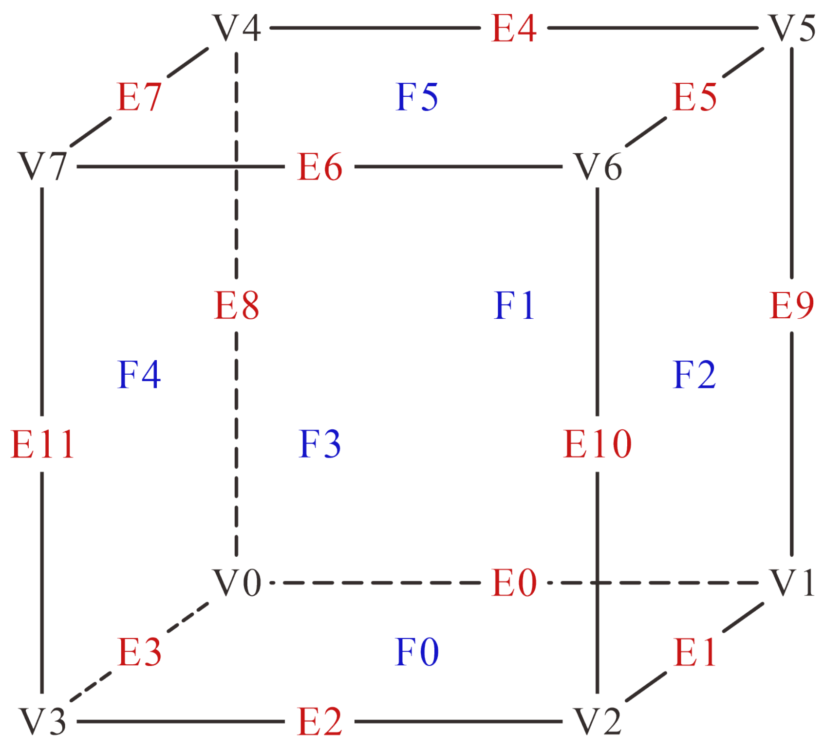
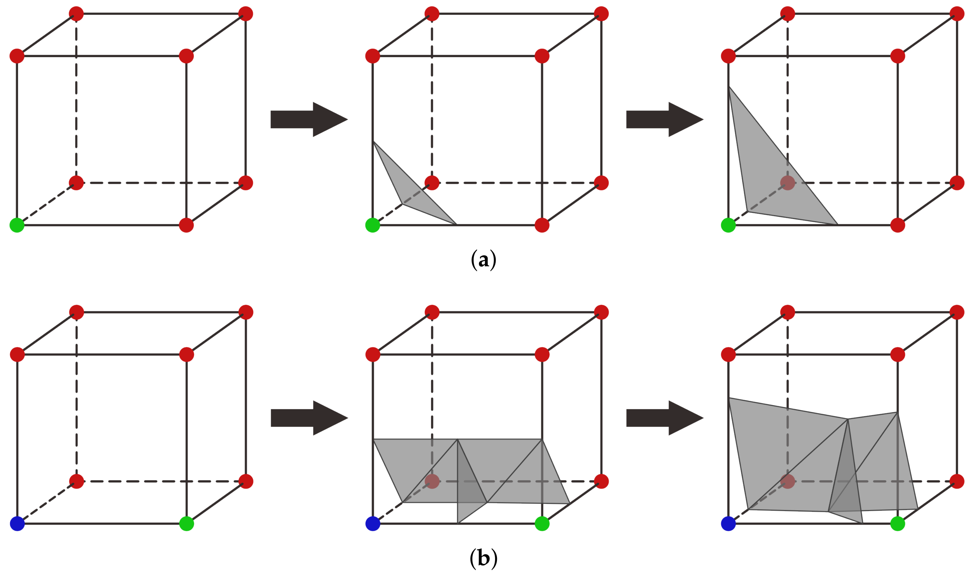
2.2. Generalized Marching Cubes Algorithm

The traditional marching cubes algorithm is limited to generating two-region interfaces, while geological interfaces may involve multi-region intersections. A generalized marching cubes algorithm is proposed to represent multi-region interfaces, with the three-region intersection used as an example.

First, the entire modeling region is discretized into a grid, with each cube in the grid computed independently. Figure 1 illustrates the spatial relationships among vertices (${\mathrm{V}}_0\sim {\mathrm{V}}_7$), edges (${\mathrm{E}}_0\sim {\mathrm{E}}_{1}1$), and faces (${\mathrm{F}}_0\sim {\mathrm{F}}_5$) within a cubic structure. As shown in, within each cube, the stratigraphy at each vertex ${\mathrm{P}}_{\mathrm{V}q}$ (where $q=0, \dots , 7$) is sequentially calculated as follows:

$$k_{\mathrm{V}q}=\underset{i}{\arg \max }\left\{f_i\left({\mathit{x}}_{\mathrm{V}q}\right)\right\}(i=1, \dots , l)$$

(10)

where ${\mathit{x}}_{\mathrm{V}q}$ is the coordinates of the vertex ${\mathrm{P}}_{\mathrm{V}q}$. In Equation (10), which is derived from Equation (3), the component of $\mathit{f}\left({\mathit{x}}_{\mathrm{V}q}\right)$ with the maximum value is identified, and its index is stored as $k_{\mathrm{V}q}$.

As shown in Figure 1, there are 18 possible intersection points in the cube: 12 edge-intersection points ${\mathrm{P}}_{\mathrm{E}0}\sim {\mathrm{P}}_{\mathrm{E}11}$, where the interfaces intersect the 12 edges of the cube, and 6 face-intersection points ${\mathrm{P}}_{\mathrm{F}0}\sim {\mathrm{P}}_{\mathrm{F}5}$, where the intersection between interfaces intersect the 6 faces of the cube. Within each cube, depending on the stratum in which each vertex is located, there may be $3^8=6561$ possible configurations. However, due to the rotational invariance of the cube and the rotational symmetry of the vertices, these configurations can be reduced to 72 unique cases. Figure 2 illustrates the triangular facets within the cube for these 72 cases, where the red, green, and blue points are vertices located in different regions, and the gray triangles simply indicate the presence of triangular facets without including coordinate information.

After determining the existence of the triangular facets, the next step is to identify the vertices of the triangles, i.e., the coordinates of all intersection points within the cube. For convenience, let ${\mathrm{P}}_{\mathrm{V}0}{\mathrm{P}}_{\mathrm{V}3}\Vert x$-axis, ${\mathrm{P}}_{\mathrm{V}0}{\mathrm{P}}_{\mathrm{V}1}\Vert y$-axis, and ${\mathrm{P}}_{\mathrm{V}0}\sim {\mathrm{P}}_{\mathrm{V}4}\Vert z$-axis.

• For the intersection points ${\mathrm{P}}_{\mathrm{E}0}\sim {\mathrm{P}}_{\mathrm{E}11}$

The calculation method for the coordinates of these points is based on Equation (4). Let the coordinates of the two vertices of an edge be ${\mathit{x}}_1$ and ${\mathit{x}}_2$, located in strata $k_1$ and $k_2$, respectively. The coordinates of the intersection point ${\mathit{x}}_{\mathrm{E}}$ are then calculated using linear interpolation. Let

$$m={\displaystyle \frac{f_{k_1}\left({\mathit{x}}_1\right)-f_{k_2}\left({\mathit{x}}_1\right)}{f_{k_1}\left({\mathit{x}}_1\right)-f_{k_2}\left({\mathit{x}}_1\right)+f_{k_1}\left({\mathit{x}}_2\right)-f_{k_2}\left({\mathit{x}}_2\right)}}.$$

(11)

For the intersection points ${\mathrm{P}}_{\mathrm{E}1}, {\mathrm{P}}_{\mathrm{E}3}, {\mathrm{P}}_{\mathrm{E}5}, {\mathrm{P}}_{\mathrm{E}7}$, the coordinates of the vertices and the intersection points are related as follows:

$$\left\{\begin{array}{cc}{\mathit{x}}_1\hfill & =(x_1, y_0, z_0)\hfill \\ {\mathit{x}}_2\hfill & =(x_2, y_0, z_0)\hfill \\ {\mathit{x}}_{\mathrm{E}}\hfill & =(x_1+m(x_2-x_1), y_0, z_0)\hfill \end{array}\right.;$$

(12)

similarly, for ${\mathrm{P}}_{\mathrm{E}0}, {\mathrm{P}}_{\mathrm{E}2}, {\mathrm{P}}_{\mathrm{E}4}, {\mathrm{P}}_{\mathrm{E}6}$, we have

$$\left\{\begin{array}{cc}{\mathit{x}}_1\hfill & =(x_0, y_1, z_0)\hfill \\ {\mathit{x}}_2\hfill & =(x_0, y_2, z_0)\hfill \\ {\mathit{x}}_{\mathrm{E}}\hfill & =(x_0, y_1+m(y_2-y_1), z_0)\hfill \end{array}\right.;$$

(13)

for ${\mathrm{P}}_{\mathrm{E}8}, {\mathrm{P}}_{\mathrm{E}9}, {\mathrm{P}}_{\mathrm{E}10}, {\mathrm{P}}_{\mathrm{E}11}$:

$$\left\{\begin{array}{cc}{\mathit{x}}_1\hfill & =(x_0, y_0, z_1)\hfill \\ {\mathit{x}}_2\hfill & =(x_0, y_0, z_2)\hfill \\ {\mathit{x}}_{\mathrm{E}}\hfill & =(x_0, y_0, z_1+m(z_2-z_1))\hfill \end{array}\right.$$

(14)

2.

For the intersection points ${\mathrm{P}}_{\mathrm{F}0}\sim {\mathrm{P}}_{\mathrm{F}5}$

The calculation method for the coordinates of these points is based on Equation (5). Let the coordinates of the four vertices of the face be ${\mathit{x}}_1, {\mathit{x}}_2, {\mathit{x}}_3, {\mathit{x}}_4$, located in three strata $k_1, k_2, k_3$, respectively. The coordinates of the intersection point ${\mathit{x}}_{\mathrm{F}}$ are then calculated using bilinear interpolation. For the intersection points ${\mathrm{P}}_{\mathrm{F}0}$ and ${\mathrm{P}}_{\mathrm{F}5}$, we have

$$\left\{\begin{array}{cc}{\mathit{x}}_1\hfill & =(x_1, y_1, z_0)\hfill \\ {\mathit{x}}_2\hfill & =(x_1, y_2, z_0)\hfill \\ {\mathit{x}}_3\hfill & =(x_2, y_2, z_0)\hfill \\ {\mathit{x}}_4\hfill & =(x_2, y_1, z_0)\hfill \\ {\mathit{x}}_{\mathrm{F}}\hfill & =(x_{\mathrm{F}}, y_{\mathrm{F}}, z_0)\hfill \end{array}\right.,$$

(15)

Bilinear interpolation is performed on $f_{k_1}, f_{k_2}, f_{k_3}$, and the result is

$${\tilde{f}}_{k_t}(x, y)=a_{t}xy+b_{t}x+c_{t}y+d_t(t=1, 2, 3),$$

(16)

where

$$\left\{\begin{array}{cc}{a}_t\hfill & ={\displaystyle \frac{f_{k_t}\left({\mathit{x}}_1\right)-f_{k_t}\left({\mathit{x}}_2\right)+f_{k_t}\left({\mathit{x}}_3\right)-f_{k_t}\left({\mathit{x}}_4\right)}{(x_2-x_1)(y_2-y_1)}}\hfill \\ b_t\hfill & ={\displaystyle \frac{-y_2{f}_{k_t}\left({\mathit{x}}_1\right)+y_1{f}_{k_t}\left({\mathit{x}}_2\right)-y_1{f}_{k_t}\left({\mathit{x}}_3\right)+y_2{f}_{k_t}\left({\mathit{x}}_4\right)}{(x_2-x_1)(y_2-y_1)}}\hfill \\ c_t\hfill & ={\displaystyle \frac{-x_2{f}_{k_t}\left({\mathit{x}}_1\right)+x_1{f}_{k_t}\left({\mathit{x}}_2\right)-x_1{f}_{k_t}\left({\mathit{x}}_3\right)+x_2{f}_{k_t}\left({\mathit{x}}_4\right)}{(x_2-x_1)(y_2-y_1)}}\hfill \\ d_t\hfill & ={\displaystyle \frac{x_2{y}_2{f}_{k_t}\left({\mathit{x}}_1\right)-x_2{y}_1{f}_{k_t}\left({\mathit{x}}_2\right)+x_1{y}_1{f}_{k_t}\left({\mathit{x}}_3\right)-x_1{y}_2{f}_{k_t}\left({\mathit{x}}_4\right)}{(x_2-x_1)(y_2-y_1)}}\hfill \end{array}\right.$$

(17)

The intersection point is located at the intersection of the stratigraphic interfaces; therefore,

$${\tilde{f}}_{k_1}(x, y)={\tilde{f}}_{k_2}(x, y)={\tilde{f}}_{k_3}(x, y).$$

(18)

This allows the problem to be transformed into a system of equations, as follows:

$$\left\{\begin{array}{cc}(a_2-a_1)x_{\mathrm{F}}{y}_{\mathrm{F}}+(b_2-b_1)x_{\mathrm{F}}+(c_2-c_1)y_{\mathrm{F}}+(d_2-d_1)\hfill & =0\hfill \\ (a_3-a_1)x_{\mathrm{F}}{y}_{\mathrm{F}}+(b_3-b_1)x_{\mathrm{F}}+(c_3-c_1)y_{\mathrm{F}}+(d_3-d_1)\hfill & =0\hfill \end{array}\right.$$

(19)

${\mathit{x}}_{\mathrm{F}}$ and ${\mathit{y}}_{\mathrm{F}}$ are obtained by solving the equations. Similarly, the coordinates of ${\mathrm{P}}_{\mathrm{F}1}, {\mathrm{P}}_{\mathrm{F}2}, {\mathrm{P}}_{\mathrm{F}3}, {\mathrm{P}}_{\mathrm{F}4}$ can also be calculated.

Figure 3 illustrates the complete modeling process of triangular facets within the cube. In Figure 3a, the first diagram identifies the stratum corresponding to the eight vertices, where ${\mathrm{P}}_{\mathrm{V}}3$ belongs to one stratum while the remaining vertices belong to another. This cube corresponds to Case 01 in Figure 2, leading to the identification of points ${\mathrm{P}}_{\mathrm{E}}2$, ${\mathrm{P}}_{\mathrm{E}}3$, and ${\mathrm{P}}_{\mathrm{E}}11$, as well as the triangular facet ${\mathrm{P}}_{\mathrm{E}}2{\mathrm{P}}_{\mathrm{E}}3{\mathrm{P}}_{\mathrm{E}}11$, as shown in the second diagram. The coordinates of ${\mathrm{P}}_{\mathrm{E}}2$, ${\mathrm{P}}_{\mathrm{E}}3$, and ${\mathrm{P}}_{\mathrm{E}}11$ are then computed, with a possible result displayed in the third diagram. Figure 3b presents the modeling process for a cube containing three strata, corresponding to Case 03 in Figure 2.

The final step is to calculate the normal vector at each vertex of the triangle. During model visualization, the rendering program will smooth the lighting effects based on the vertex normal vectors, resulting in a high degree of smoothness. Let ${\mathit{x}}^{\prime }$ be an arbitrary point on the interface between strata $k_1$ and $k_2$. The normal vector at each vertex is

$${\mathit{n}}^{\prime }=\sum _{j=1}^n({\mathbf{\lambda }}_{j{k}_1}-{\mathbf{\lambda }}_{j{k}_2}){\displaystyle \frac{{\mathit{x}}^{\prime }-{\mathit{x}}_j}{\sqrt{{∥{\mathit{x}}^{\prime }-{\mathit{x}}_j∥}^2+c^2}}}$$

(20)

2.3. Modeling Process

The modeling process is shown in Figure 4. Control points at the interfaces are obtained from borehole data, and points within the strata are inserted based on these control points. The coordinates and potential vector values of both control and inserted points form a dataset. Radial basis function interpolation is then applied to obtain the potential vector field for the entire study area. The region is discretized into a regular cubic grid, and the potential vector values at all cube vertices are calculated. Finally, a 3D geological model is generated using the generalized marching cubes algorithm.

We use a mineral deposit area as the study area, with an east–west length of 6112.8 m and a north–south length of 13,310.2 m. A total of 100 borehole data points were collected, and the region was divided into five stratigraphic layers. The distribution of the boreholes is shown in Figure 5. Different strata are represented by distinct colors in the boreholes. The borehole depths are much smaller than the horizontal span of the region, so the z-axis is scaled proportionally by a factor of $A=10$ to enhance the visual representation of both the borehole data and the final modeling results.

Throughout the modeling process, the key issues addressed are as follows:

• Data Point Acquisition from Borehole Data

The borehole data for the study area includes the following: (a) Basic borehole information: This dataset records the geographical location and depth information of each borehole, including geodetic coordinates, borehole elevation, and borehole depth. (b) Borehole stratification information: This dataset records the depth information of the strata within each borehole, including the starting depth and the ending depth of each layer.

As shown in Figure 6, the data points located at the stratigraphic interface are control points that can be directly obtained from borehole data, represented by red points. The data points located within the strata are inserted between the control points, represented by blue points. The coordinates of the control points, ${\mathit{x}}_r=(x_r, y_r, z_r)$, can be expressed as

$$\left\{\begin{array}{cc}{x}_r\hfill & =X\hfill \\ y_r\hfill & =Y\hfill \\ z_r\hfill & =Z-D\hfill \end{array}\right.,$$

(21)

where X and Y represent the geographic coordinates of the borehole, Z denotes the elevation at the borehole mouth, and D refers to the depth of the control point, expressed using either the starting or reaching depth of the stratum. A series of data points with equal spacing are inserted between adjacent control points, and the specific number of these data points, denoted as $n_a$, is

$$n_{\mathrm{a}}=\max \left\{⌈{\displaystyle \frac{d_{\mathrm{a}}}{d_{\max }}}⌉-1, n_{\min }\right\},$$

(22)

where $d_{\mathrm{a}}$ is the distance between two adjacent control points, while $d_{\max }$ and $n_{\min }$ need to be specified based on actual conditions. $d_{\max }$ is the maximum distance between data points, and $n_{\min }$ is the minimum number of data points between two control points. The data points between two control points are spaced at equal intervals, given by

$$d={\displaystyle \frac{d_{\mathrm{a}}}{n_{\mathrm{a}}+1}}$$

(23)

Between two control points, there are relationships given by

$$\left\{\begin{array}{cc}{n}_{\mathrm{a}}>n_{\min }\hfill & (d_a>(n_{\min }+1)d_{\max })\hfill \\ n_{\mathrm{a}}=n_{\min }\hfill & (d_a\le (n_{\min }+1)d_{\max })\hfill \end{array}\right.,$$

(24)

$$\left\{\begin{array}{cc}{\displaystyle \frac{n_{\min }}{n_{\min }+1}}{d}_{\max }<d\le d_{\max }\hfill & (d_a>(n_{\min }+1)d_{\max })\hfill \\ d=d_{\max }\hfill & (d_a=(n_{\min }+1)d_{\max })\hfill \\ 0<d<d_{\max }\hfill & (d_a<(n_{\min }+1)d_{\max })\hfill \end{array}\right.$$

(25)

This ensures that the distance between data points in thick strata remains within a relatively defined range. In thin strata, a fixed number of data points is used. This approach prevents the data points from being too sparse, which could adversely affect the modeling accuracy, or too dense, which would lead to unnecessary computational overhead.

2.

Constructing a Potential Vector Field

The potential vector field values at all control points and insertion points are calculated using Equation (1). A dataset of data points ${\{{\mathit{x}}_i, {\mathit{s}}_i\}}_{i=1}^n$, containing coordinates and potential vector values, is constructed. The interpolation function $\mathit{f}\left(\mathit{x}\right)$, as shown in Equation (6), is sought by substituting the data points into the interpolation constraints, resulting in the linear system of equations represented by Equation (8). By solving this system, the unknown coefficients in Equation (6) are determined, and the resulting $\mathit{f}\left(\mathit{x}\right)$ is the desired potential vector field.

3.

Generating a Geological Surface Model

After obtaining the potential vector field function, the entire study area is divided into a regular cubic grid, with the grid size being determined according to practical requirements. The potential vector field values are then calculated at the intersection points of the grid. Subsequently, within each cube, triangular facets are obtained using the generalized marching cubes algorithm, and the vertex normal vectors of the triangles are computed using Equation (20). This process achieves illumination smoothing, and the collection of all triangular facets forms the final geological surface model.

4.

GPU Parallel Processing

Traditional methods for solving linear systems of equations have a time complexity of $O\left(n^3\right)$. When using a CPU to solve Equation (8), the computation time increases rapidly as the number of data points grows. For example, when the number of data points reaches several thousand, the solution process may take several hours. The GPU is a hardware platform designed for performing large-scale parallel computations, with hundreds or even thousands of processing cores. Based on the single instruction, multiple threads (SIMT) architecture, it enables efficient parallel computation using thread blocks. Many researchers have studied the parallel solution of large linear systems using GPUs [30,31,32]. In this paper, the LU decomposition API provided by the CUBLAS library is utilized to accelerate the solution of the linear system, thereby improving modeling efficiency.

3. Results

The modeling program was developed using the C++ programming language. The experimental environment was as follows:

• CPU: Intel(R) Core(TM) i5-8300H CPU 2.30 GHz (Intel Corporation, Santa Clara, CA, USA); Procurement Source: Dell(China) Inc., Xiamen, China.
• GPU: NVIDIA GeForce GTX 1050 (2.0 GB) (NVIDIA Corporation, Santa Clara, CA, USA); Procurement Source: Dell(CHina) Inc., Xiamen, China.;
• Memory: 8.0 GB.

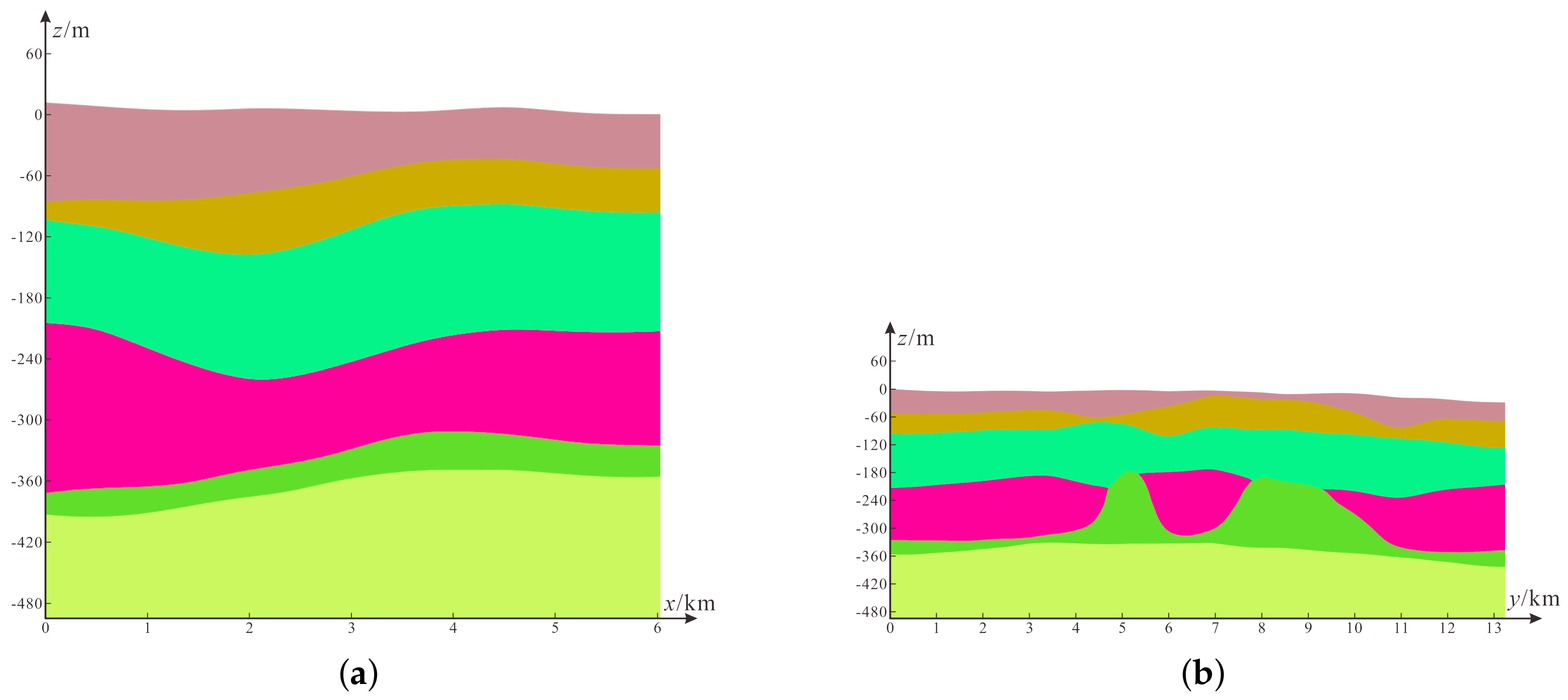
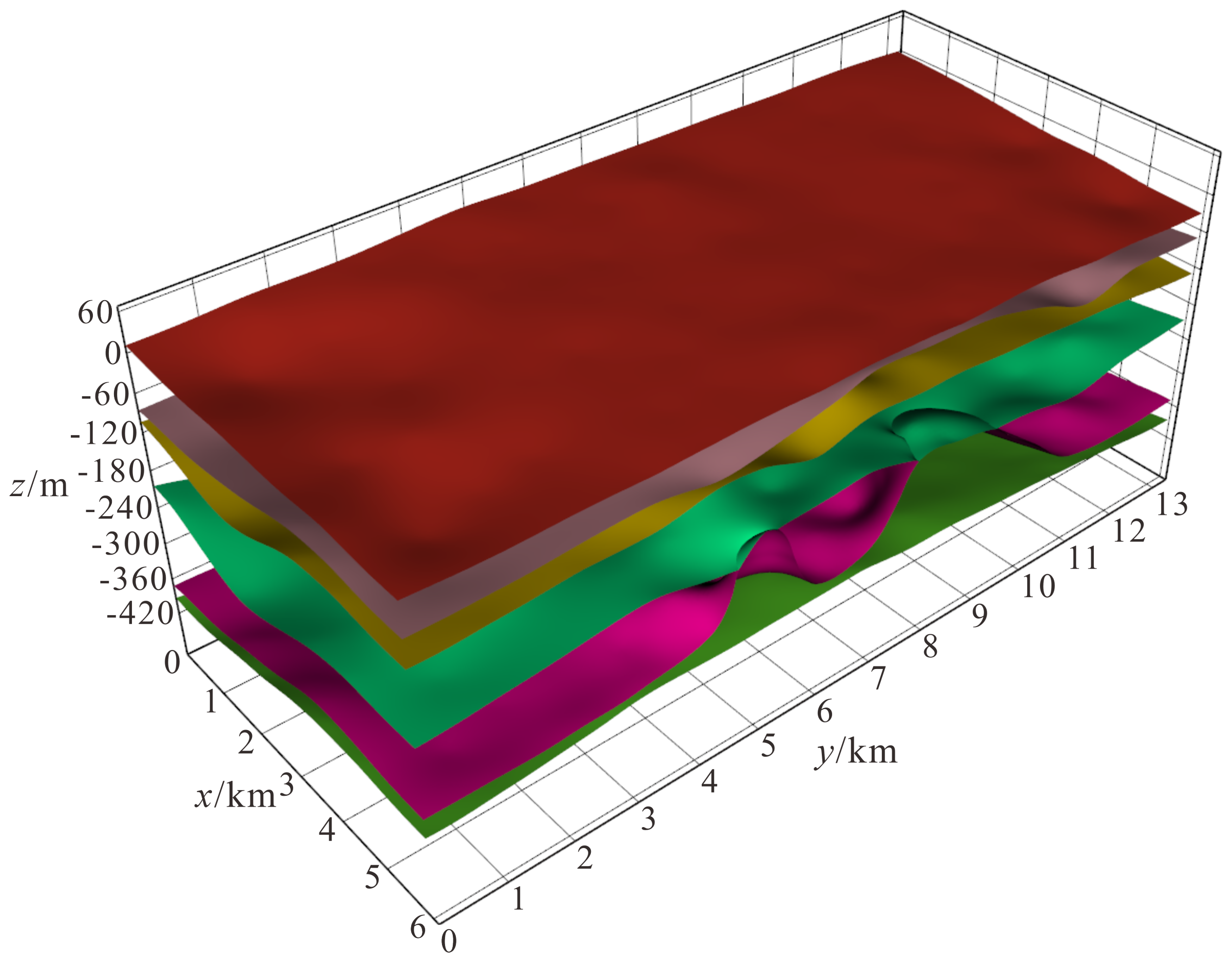
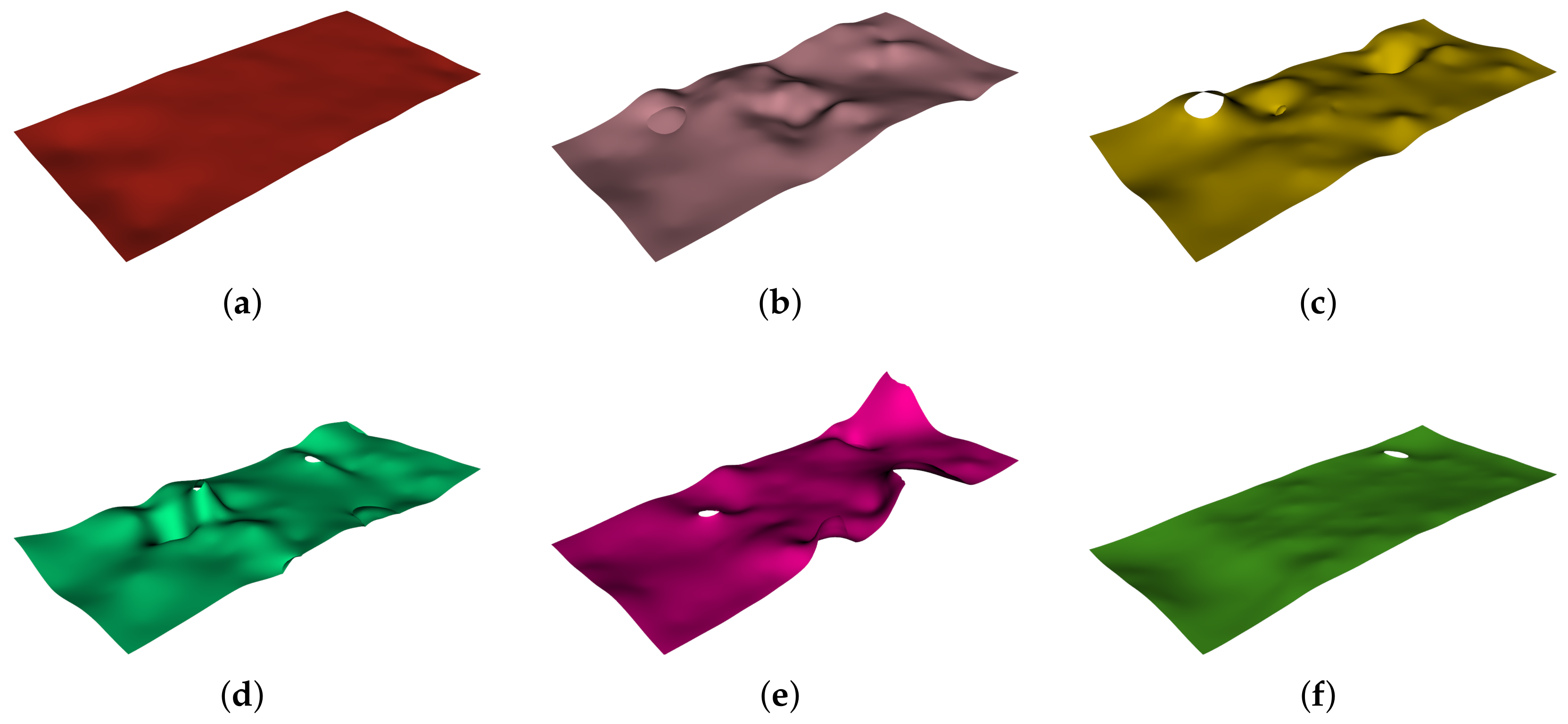
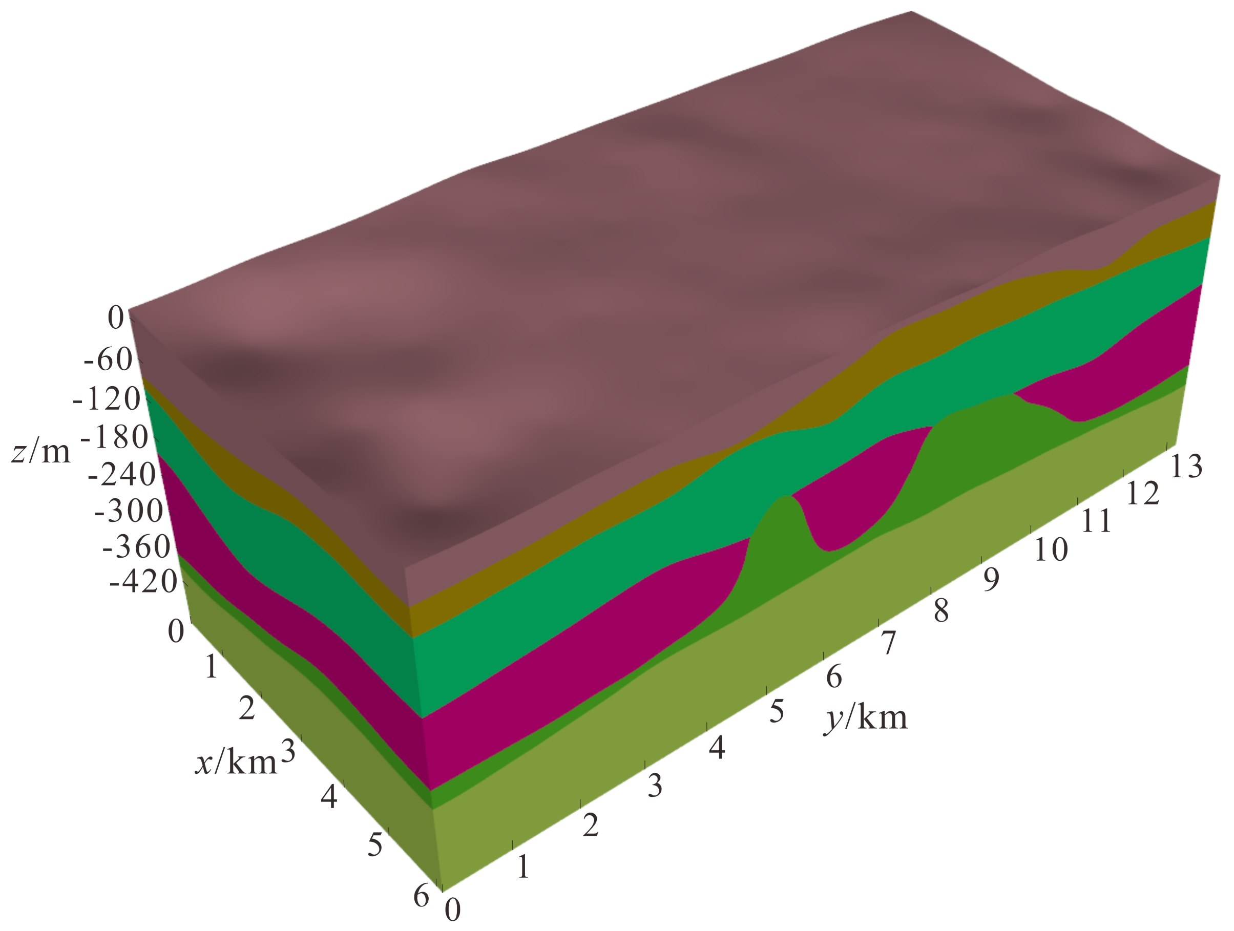
3.1. Geological Model Visualization Results

The parameters selected for the experiment were $c=10$, $d_{\max }=10\mathrm{m}$, $n_{\min }=5$, with a grid size of $90\mathrm{m}\times 90\mathrm{m}\times 3\mathrm{m}$. The resulting dataset contained 7306 data points, and the total number of cubes was 1,892,032.

Figure 7 presents the two-dimensional cross-sectional view along the x and y axes, where the intersection at the stratigraphic interfaces exhibiting erosion phenomena is correctly represented, with no topological errors. Figure 8 shows the visualization of the geological interface set, which includes 113,327 data points and 221,763 triangular facets. Figure 9 illustrates the results of different geological interfaces, where the interfaces in panels (c), (d), (e), and (f) exhibit partial missing sections, due to erosion occurring in the corresponding stratigraphic areas. Figure 10 displays the local geological interfaces where erosion phenomena are present. Figure 11 provides the full view generated from the geological interfaces. From the visualizations, it is evident that the experiment successfully produced consistent unconformable geological interfaces without any topological errors, thereby validating the effectiveness of the proposed method.

3.2. Influence of Parameters

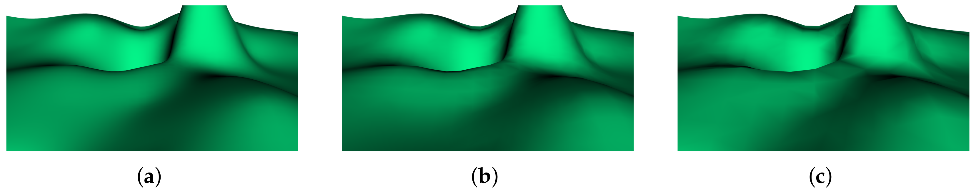
3.2.1. Influence of Grid Size

The rendering program performs smoothing of the triangular facets using vertex normal vectors without considering the influence of adjacent triangles. If the angle between adjacent triangles is too large, poor smoothing effects may occur at the junction. Figure 12 shows the local geological interfaces for grid sizes of $90\mathrm{m}\times 90\mathrm{m}\times 3\mathrm{m}$, $180\mathrm{m}\times 180\mathrm{m}\times 6\mathrm{m}$, and $270\mathrm{m}\times 270\mathrm{m}\times 9\mathrm{m}$, with average angles between adjacent triangles of 3.30°, 6.43°, and 9.29°, respectively. By reducing the grid size, the angle between adjacent triangles can be minimized, resulting in better smoothing effects. It is recommended that the average angle between adjacent triangles not exceed 5°.

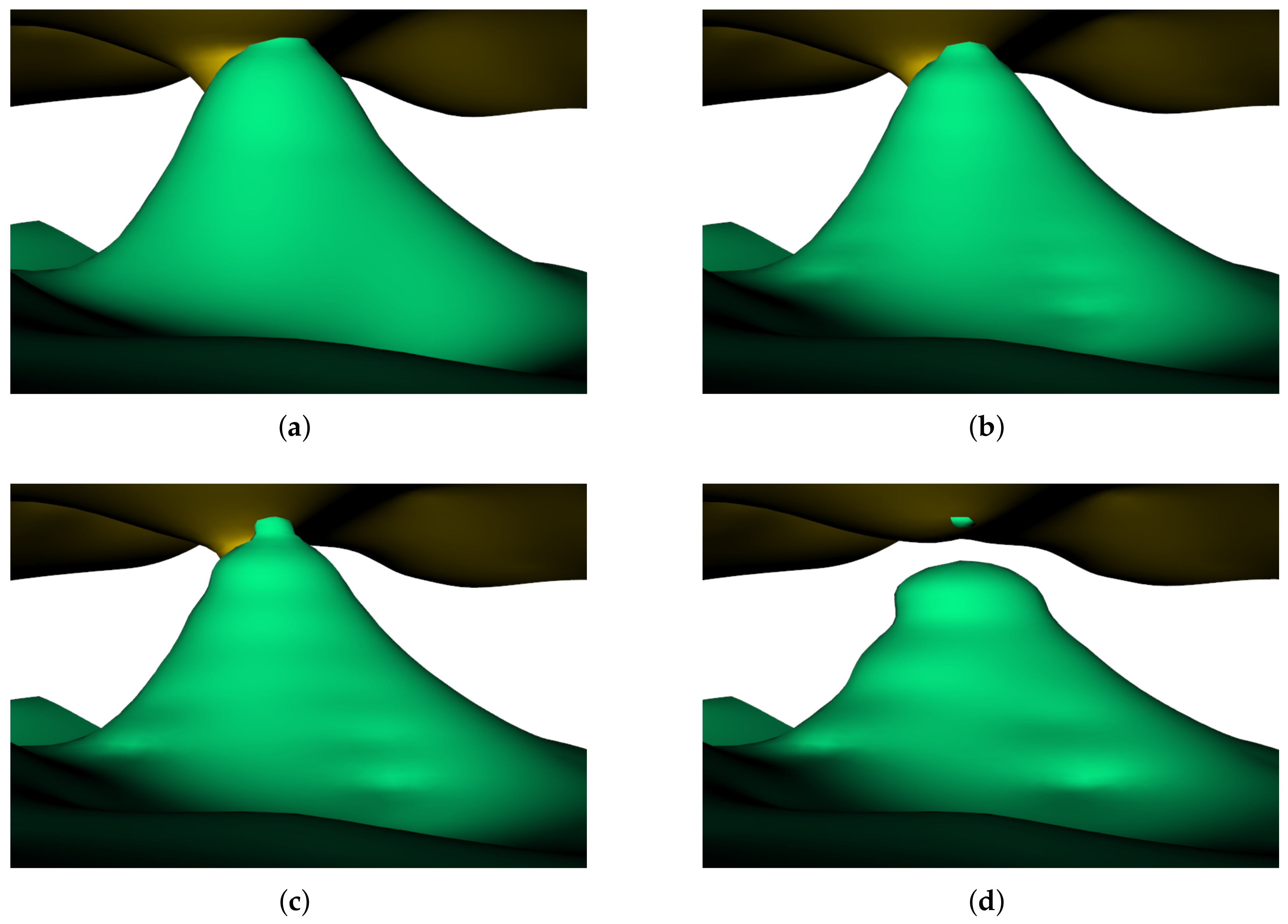
3.2.2. Influence of Data Point Spacing

The parameter $d_{\max }$ controls the maximum spacing between data points. Figure 13 shows the local geological interfaces when $n_{\min }=5$ and $c=10$, with $d_{\max }$ set to 10 m, 15 m, 20 m, and 25 m, respectively. In contrast to the geological interface shown in Figure 13a, the interfaces in Figure 13b–d exhibit noticeable undulating distortion at higher slopes. This is because a larger data point spacing leads to sparse data points in the z-axis direction, resulting in an unreasonable potential vector field. Based on experimental comparisons, it is recommended that $d_{\max }\le 1.0c$ to achieve higher-quality geological interfaces, with the shape parameter c selected according to references [33,34,35].

3.3. Validation of Model Accuracy

To evaluate the quality of the constructed 3D geological model, this study employs the leave-one-out cross-validation (LOOCV) method. Specifically, 99 out of the total 100 borehole datasets are used as the training set to construct the 3D geological model, while the remaining borehole is used as the test set. The model then predicts the depth values of stratigraphic interfaces at the test borehole location. Finally, the predicted values are compared with the true values obtained directly from the original data using quantitative error assessment metrics. To minimize randomness, all borehole data are included in the validation process. Three quantitative metrics, namely mean absolute error (MAE), root mean square error (RMSE), and Lin’s concordance correlation coefficient (CCC), are employed for evaluation, with the results being presented in

Table 1. Result of LOOCV.

Interface	MAE	RMSE	CCC
Ground surface	3.791	5.155	0.948
Base of the first stratum	7.691	9.296	0.866
Base of the second stratum	11.456	14.695	0.783
Base of the third stratum	12.578	15.901	0.758
Base of the fourth stratum	14.346	17.380	0.707
Base of the fifth stratum	3.272	5.095	0.987

. The results indicate that the model achieves an accuracy level suitable for practical applications. Moreover, the modeling accuracy for relatively flat stratigraphic interfaces is significantly higher than that for inclined interfaces. This discrepancy arises due to the limited availability of borehole data in regions with complex topography and specific drilling constraints, which negatively impacts the accuracy of certain stratigraphic interface models. To enhance the quality of the 3D geological model, future work may consider integrating multi-source data to impose additional constraints, thereby improving modeling accuracy.

3.4. GPU Acceleration Verification

To evaluate the acceleration effect of the GPU on modeling, the time required to solve the linear system of equations using the LU decomposition algorithm was tested under both CPU and GPU environments for different data point scales. The results are shown in

Table 2. Time consumption for solving the system using CPU and GPU at different data point scales.

Number of Data Points	CPU Time Consumption	GPU Time Consumption
2000	59.5 min	3.2 s
4000	7.4 h	14.9 s
6000	23.2 h	28.3 s
8000	50.7 h	49.2 s

. It can be observed that when the number of data points reaches several thousand, the CPU takes several hours, or even tens of hours, to solve the linear system. Thus, it becomes the bottleneck of the entire model generation process, which is unacceptable in practical applications. In contrast, the GPU can complete the solution in just a few seconds, achieving a solution speed more than 1000 times faster than the CPU. This significantly improves computational efficiency and enhances the adaptability of the proposed method when handling large-scale datasets.

4. Conclusions

Traditional implicit modeling methods based on potential fields cannot directly represent unconformable stratigraphic interfaces. This paper proposes a potential vector field method combined with the generalized marching cubes algorithm to achieve accurate modeling of unconformable stratigraphic interfaces. The potential vector field method uses the distance of a point in the vertical direction to the closest of two stratigraphic interfaces as a component, which introduces a new representation for unconformable stratigraphic interfaces. The generalized marching cubes algorithm extends the traditional algorithm to multi-region interfaces, constructing all possible cubes that can occur in multi-region cases, thus enabling surface generation when multiple regions meet in unconformable stratigraphic interfaces. Using actual borehole data, the paper models and visualizes surfaces that include unconformable stratigraphic interfaces, resulting in a consistent 3D geological surface model with no topological errors, thereby validating the effectiveness of the proposed method.

References

1. Wijns, C.; Boschetti, F.; Moresi, L. Inverse modelling in geology by interactive evolutionary computation. J. Struct. Geol. 2003, 25, 1615–1621. [Google Scholar] [CrossRef]
2. Madsen, R.B.; Høyer, A.S.; Andersen, L.T.; Møller, I.; Hansen, T.M. Geology-driven modeling: A new probabilistic approach for incorporating uncertain geological interpretations in 3D geological modeling. Eng. Geol. 2022, 309, 106833. [Google Scholar] [CrossRef]
3. Wang, X.; Guo, J.; Fu, S.; Zhang, H.; Liu, S.; Zhang, X.; Liu, Z.; Dun, L. Towards automatic and rapid 3D geological modelling of urban sedimentary strata from a large amount of borehole data using a parallel solution of implicit equations. Earth Sci. Inform. 2024, 17, 421–440. [Google Scholar]
4. Guo, J.; Wang, J.; Wu, L.; Liu, L.; Li, C.; Li, F.; Lin, M.; Jessell, M.W.; Li, P.; Dai, X.; et al. Explicit-implicit-integrated 3-D geological modelling approach: A case study of the Xianyan Demolition Volcano (Fujian, China). Tectonophysics 2020, 795, 228648. [Google Scholar] [CrossRef]
5. Yang, H.Q.; Chu, J.; Wu, S.; Zhu, X.; Qi, X.; Chiam, K. Advancing geological modelling and geodata management: A web-based system with AI assessment in Singapore. Georisk 2024, 19, 218–232. [Google Scholar] [CrossRef]
6. Thorleifson, H.; Berg, R.C.; Russell, H.A.J. Geological mapping goes 3-D in response to societal needs. GSA Today 2010, 20, 27–29. [Google Scholar] [CrossRef]
7. Martin-Izard, A.; Arias, D.; Arias, M.; Gumiel, P.; Sanderson, D.J.; Castañon, C.; Lavandeira, A.; Sanchez, J. A new 3D geological model and interpretation of structural evolution of the world-class Rio Tinto VMS deposit, Iberian Pyrite Belt (Spain). Ore Geol. Rev. 2015, 71, 457–476. [Google Scholar] [CrossRef]
8. Ming, J.; Pan, W.; Qu, H.; Ge, Z. GSIS: A 3D geological multi-body modeling system from netty cross-sections with topology. Comput. Geosci. 2010, 36, 756–767. [Google Scholar]
9. Guo, J.; Wu, L.; Zhou, W.; Li, C.; Li, F. Section-constrained local geological interface dynamic updating method based on the HRBF surface. J. Struct. Geol. 2018, 107, 64–72. [Google Scholar] [CrossRef]
10. González-Garcia, J.; Jessell, M. A 3D geological model for the Ruiz-Tolima Volcanic Massif (Colombia): Assessment of geological uncertainty using a stochastic approach based on Bézier curve design. Tectonophysics 2016, 687, 139–157. [Google Scholar]
11. Cowan, E.J.; Beatson, R.K.; Ross, H.J.; Fright, W.R.; McLennan, T.J.; Evans, T.R.; Carr, J.C.; Lane, R.J.; Bright, D.V.; Gillman, A.J.; et al. Practical implicit geological modelling. In Proceedings of the 5th International Mining Geology Conference, Bendigo, VIC, Australia, 17–19 November 2003. [Google Scholar]
12. Vollgger, S.A.; Cruden, A.R.; Cowan, J.E. 3D implicit geological modelling of a gold deposit from a structural geologist’s point of view. In Proceedings of the 12th SGA Biennial Meeting—Mineral Deposit Research for a High-Tech World, Uppsala, Sweden, 12–15 August 2013. [Google Scholar]
13. Calcagno, P.; Chilès, J.P.; Courrioux, G.; Guillen, A. Geological modelling from field data and geological knowledge: Part I. Modelling method coupling 3D potential-field interpolation and geological rules. Phys. Earth Planet. Inter. 2008, 171, 147–157. [Google Scholar]
14. Guo, F.; Zheng, B.; Qi, S.; Li, H.; Zhu, H.; Yue, Y.; Xie, H. A review of 3D geological modeling technology and methods. J. Eng. Geol. 2024, 32, 1143–1153. (In Chinese) [Google Scholar]
15. Li, J.; Liu, P.; Wang, X.; Cui, H.; Ma, Y. 3D geological implicit modeling method of regular voxel splitting based on layered interpolation data. Sci. Rep. 2022, 12, 13840. [Google Scholar] [CrossRef] [PubMed]
16. Wang, J.; Zhao, H.; Bi, L.; Wang, L. Implicit 3D modeling of ore body from geological boreholes data using hermite radial basis functions. Minerals 2018, 8, 443. [Google Scholar] [CrossRef]
17. Zhong, D.; Wang, L.; Bi, L.; Jia, M. Implicit modeling of complex orebody with constraints of geological rules. T. Nonferr. Metal. Soc. 2019, 29, 2392–2399. [Google Scholar]
18. Wilde, B.J.; Deutsch, C.V. Kriging and simulation in presence of stationary domains: Developments in boundary modeling. In Proceedings of the Geostatistics Oslo 2012, Oslo, Norway, 11–15 June 2012. [Google Scholar]
19. Pereira, P.E.C.; Rabelo, M.N.; Ribeiro, C.C.; Diniz-Pinto, H.S. Geological modeling by an indicator kriging approach applied to a limestone deposit in Indiara city-Goiás. REM Int. Eng. J. 2017, 70, 331–337. [Google Scholar]
20. Chen, G.; Zhu, J.; Qiang, M.; Gong, W. Three-dimensional site characterization with borehole data—A case study of Suzhou area. Eng. Geol. 2018, 234, 65–82. [Google Scholar]
21. Pakyuz-Charrier, E.; Lindsay, M.; Ogarko, V.; Giraud, J.; Jessell, M. Monte Carlo simulation for uncertainty estimation on structural data in implicit 3-D geological modeling, a guide for disturbance distribution selection and parameterization. Solid Earth 2018, 9, 385–402. [Google Scholar]
22. Macêdo, I.; Gois, J.P.; Velho, L. Hermite radial basis functions implicits. Comput. Graph. Forum 2011, 30, 27–42. [Google Scholar]
23. Guo, J.; Wang, J.; Wu, L.; Zhu, W.; Jessell, M.; Li, C.; Li, F.; Hu, H. Automatic and dynamic updating of three-dimensional ore body models from borehole and excavation data using the implicit function HRBF. Ore Geol. Rev. 2022, 148, 105018. [Google Scholar]
24. Zhang, Q.; Zhu, H. Collaborative 3D geological modeling analysis based on multi-source data standard. Eng. Geol. 2018, 246, 233–244. [Google Scholar] [CrossRef]
25. Vollgger, S.A.; Cruden, A.R.; Ailleres, L.; Cowan, E.J. Regional dome evolution and its control on ore-grade distribution: Insights from 3D implicit modelling of the Navachab gold deposit, Namibia. Ore Geol. Rev. 2015, 69, 268–284. [Google Scholar] [CrossRef]
26. Guo, J.; Wang, X.; Wang, J.; Dai, X.; Wu, L.; Li, C.; Li, F.; Liu, S.; Jessell, M.W. Three-dimensional geological modeling and spatial analysis from geotechnical borehole data using an implicit surface and marching tetrahedra algorithm. Eng. Geol. 2021, 284, 106047. [Google Scholar] [CrossRef]
27. Lorensen, W.E.; Cline, H.E. Marching cubes: A high resolution 3D surface construction algorithm. In Seminal Graphics: Pioneering Efforts that Shaped the Field; Association for Computing Machinery: New York, NY, USA, 1998; pp. 347–353. [Google Scholar]
28. Guéziec, A.; Hummel, R. Exploiting triangulated surface extraction using tetrahedral decomposition. IEEE Trans. Vis. Comput. Graph. 1995, 1, 328–342. [Google Scholar] [CrossRef]
29. Wang, M.; Feng, J.; Yang, B. Comparison and Evaluation of Marching Cubes and Marching Tetrahedra. J. Comput. Aided Des. Comput. Graph. 2014, 26, 2099–2106. (In Chinese) [Google Scholar]
30. Nico, G. LU-GPU: Efficient algorithms for solving dense linear systems on graphics hardware. In Proceedings of the SC’05: Proceedings of the 2005 ACM/IEEE Conference on Supercomputing, Seattle, WA, USA, 12–18 November 2005. [Google Scholar]
31. Volkov, V.; Demmel, J. LU, QR and Cholesky Factorizations Using Vector Capabilities of GPUs. 2008. Available online: https://bebop.cs.berkeley.edu/pubs/volkov2008-gpu-factorizations.pdf (accessed on 14 January 2025).
32. Agullo, E.; Augonnet, C.; Dongarra, J.; Faverge, M.; Ltaief, H.; Thibault, S.; Tomov, S. QR Factorization on a Multicore Node Enhanced with Multiple GPU Accelerators. In Proceedings of the 2011 IEEE International Parallel & Distributed Processing Symposium, Anchorage, AK, USA, 16–20 May 2011. [Google Scholar]
33. Hardy, R.L. Multiquadric equations of topography and other irregular surfaces. J. Geophys. Res. 1971, 76, 1905–1915. [Google Scholar] [CrossRef]
34. Franke, R. Scattered data interpolation: Tests of some methods. Math. Comput. 1982, 38, 181–200. [Google Scholar]
35. Foley, T.A. Interpolation and approximation of 3-D and 4-D scattered data. Comput. Math. Appl. 1987, 13, 711–740. [Google Scholar] [CrossRef]
Figure 1. The positional relationship between the vertices and the intersection points.
Applsci 15 03594 g001
Figure 2. Depiction of 72 cases with vertices and internal triangular facets.
Applsci 15 03594 g002
Figure 3. Triangular facets modeling process. (a) Case 01 in Figure 2. (b) Case 03 in Figure 2.
Applsci 15 03594 g003
Figure 4. Modeling flowchart.
Applsci 15 03594 g004
Figure 5. Borehole distribution map of the study area.
Applsci 15 03594 g005
Figure 6. The schematic diagram of the data points is determined based on the borehole data.
Applsci 15 03594 g006
Figure 7. Two-dimensional sectional model in different directions. (a) Longitudinal section along the x-axis. (b) Longitudinal section along the y-axis.
Applsci 15 03594 g007
Figure 8. Geological interface set of the study area.
Applsci 15 03594 g008
Figure 9. Various geological interfaces in the study area. (a) Ground surface. (b) Base of the first stratum. (c) Base of the second stratum. (d) Base of the third stratum. (e) Base of the fourth stratum. (f) Base of the fifth stratum.
Applsci 15 03594 g009
Figure 10. Local geological interfaces with erosion phenomena in the study area. (a) Erosion zone at the boundary of the study area. (b) Erosion zone within the study area.
Applsci 15 03594 g010
Figure 11. Overall view of the 3D geological model of the study area (derived from geological interfaces).
Applsci 15 03594 g011
Figure 12. Local geological interfaces at different grid sizes: (a) 90 m × 90 m × 3 m; (b) 180 m × 180 m × 6 m; (c) 270 m × 270 m × 9 m.
Applsci 15 03594 g012
Figure 13. Geological interface set and local geological interfaces at different d max values when n min = 5 . (a) d max = 10 m . (b) d max = 15 m . (c) d max = 20 m . (d) d max = 25 m .
Applsci 15 03594 g013