
Entropy-Driven Adaptive Neighborhood Selection and Fitting for Sub-Millimeter Defect Detection and Quantitative Evaluation in Magnetic Tiles


Abstract
1. Introduction
1.1. Problem Statement
1.2. Related Work
1.2.1. Methods Based on 2D Images
1.2.2. Methods Based on 3D Point Clouds
1.3. Our Contributions
- Combining the improved weighted covariance matrix and information entropy, the accuracy of defect detection is enhanced while reducing the need for extensive feature engineering.
- Leveraging luminance and point cloud mapping (LPM), the ability to identify potential defects is enhanced.
- Combining single-frame and multi-frame point cloud fitting reduces false detection rates, minimizes reliance on feature engineering, and aids in effective defect assessment.
2. Materials
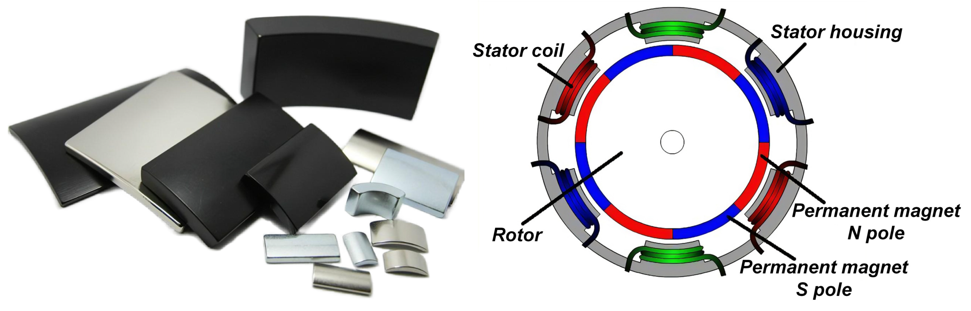
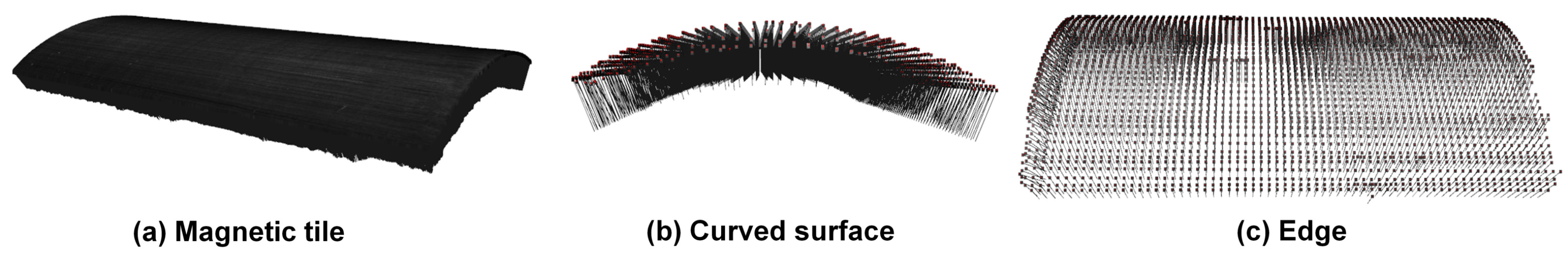
2.1. Magnetic Tiles
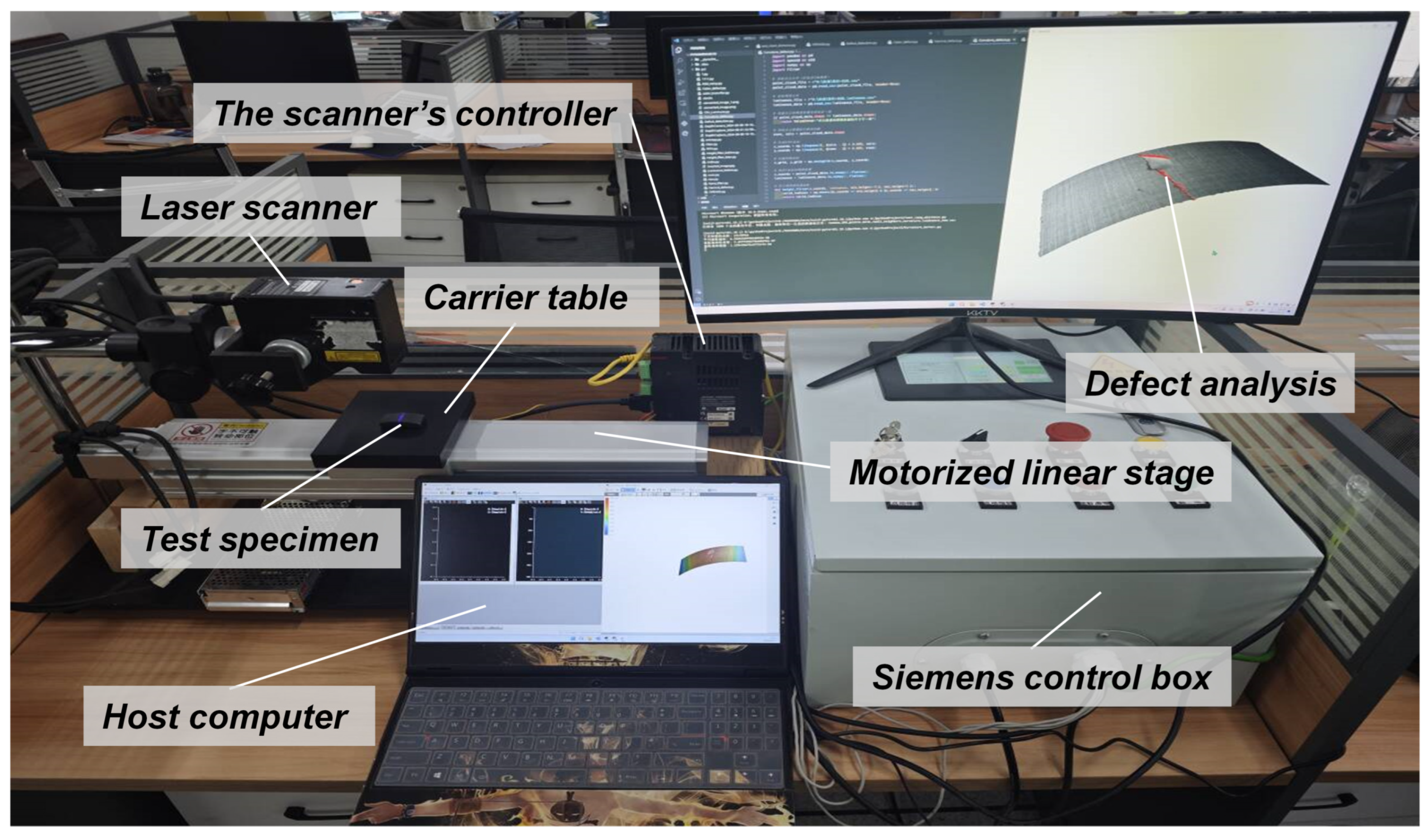
2.2. System Setup
2.3. Experimental Data
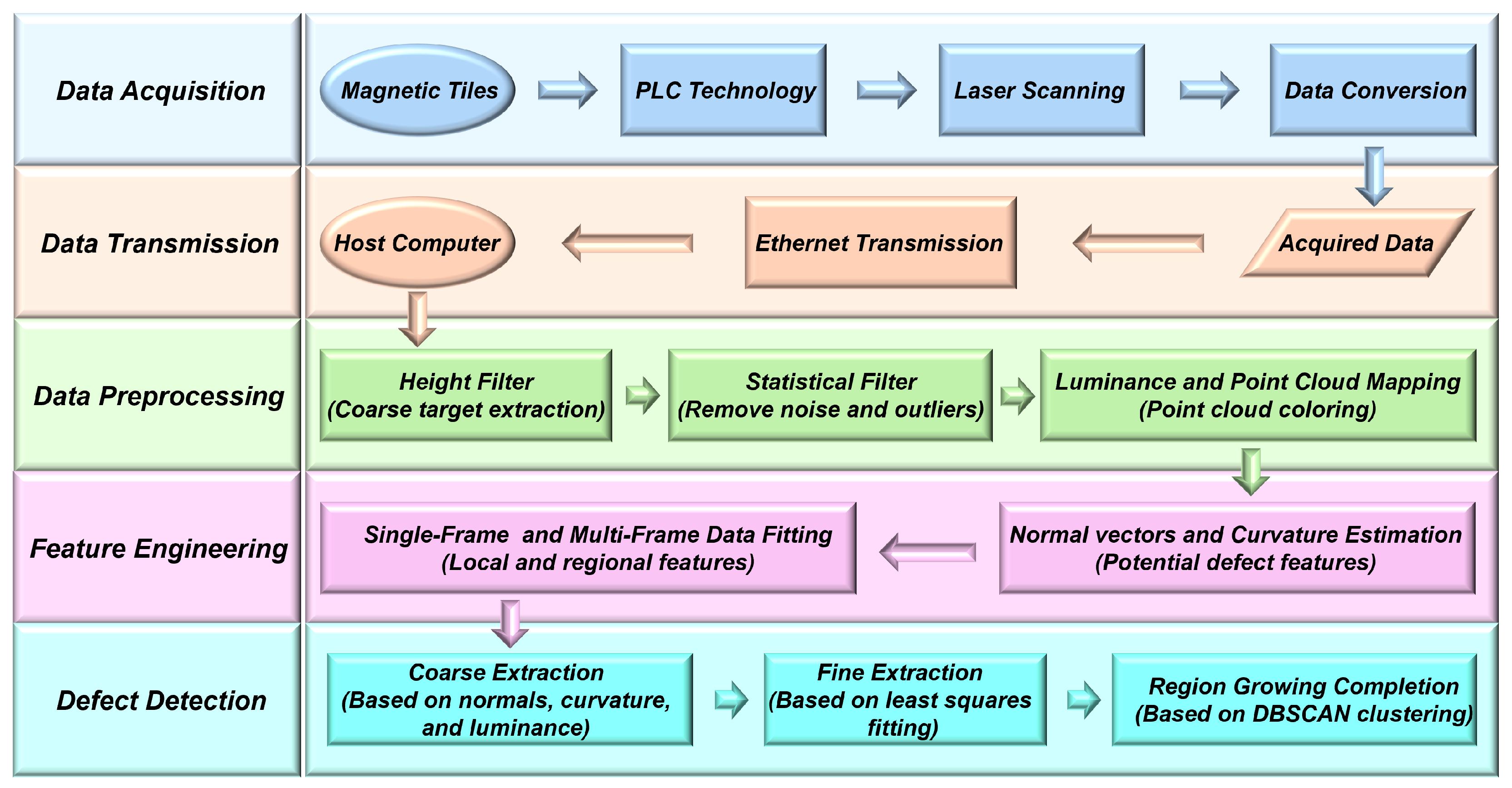
3. Methodology
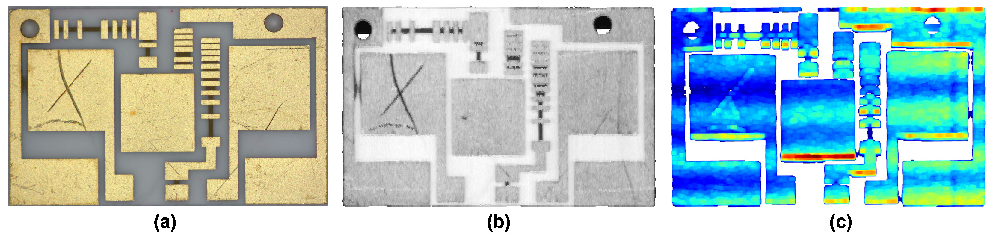
3.1. Height-Based Target Extraction
3.2. Outlier and Extraneous Point Removal
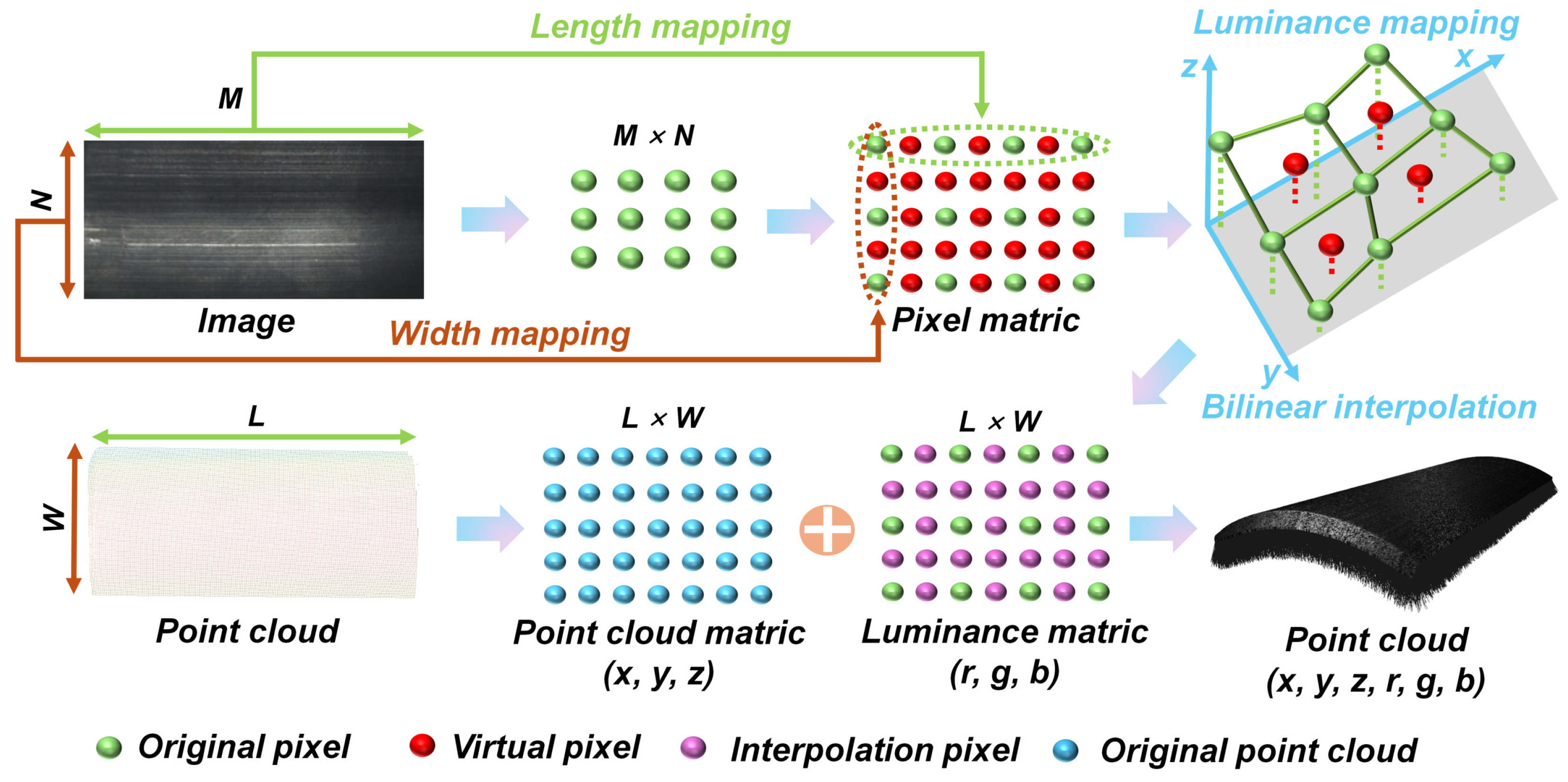
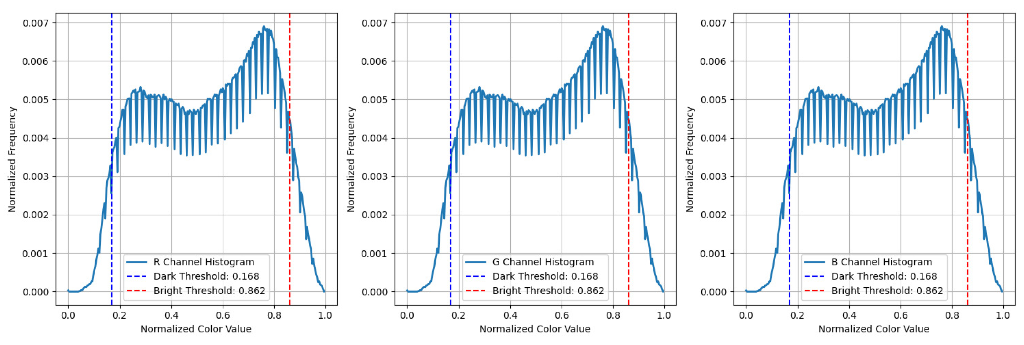
3.3. Luminance and Point Cloud Mapping
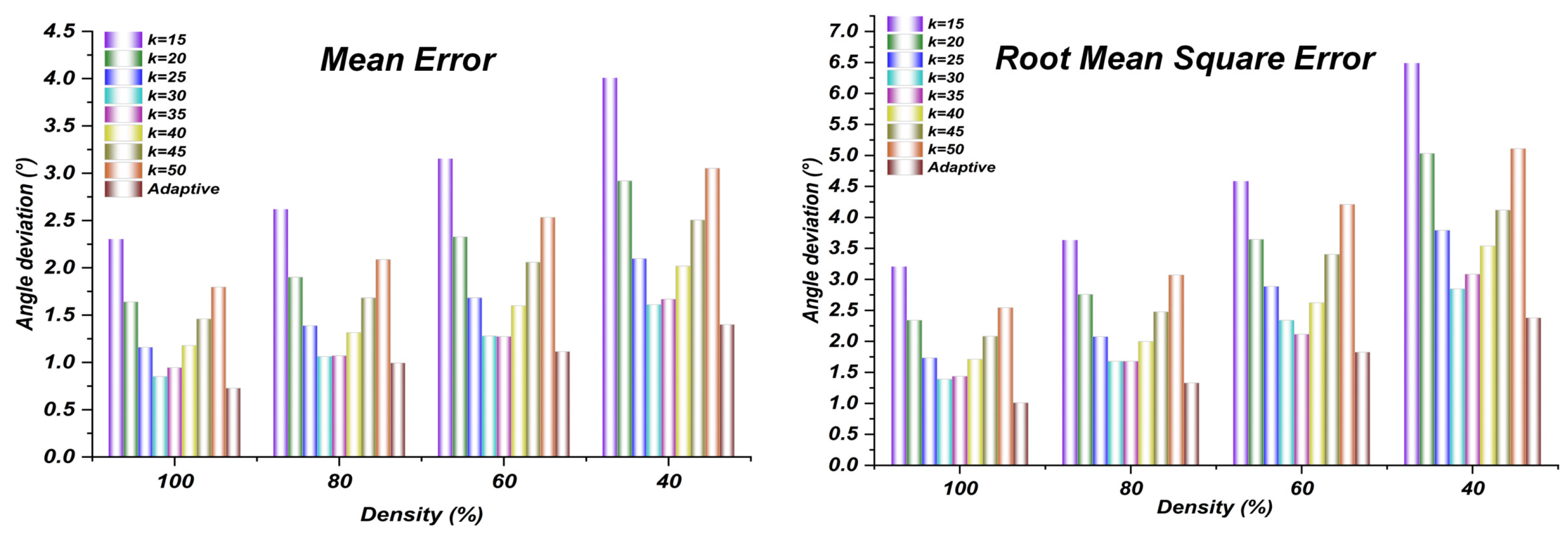
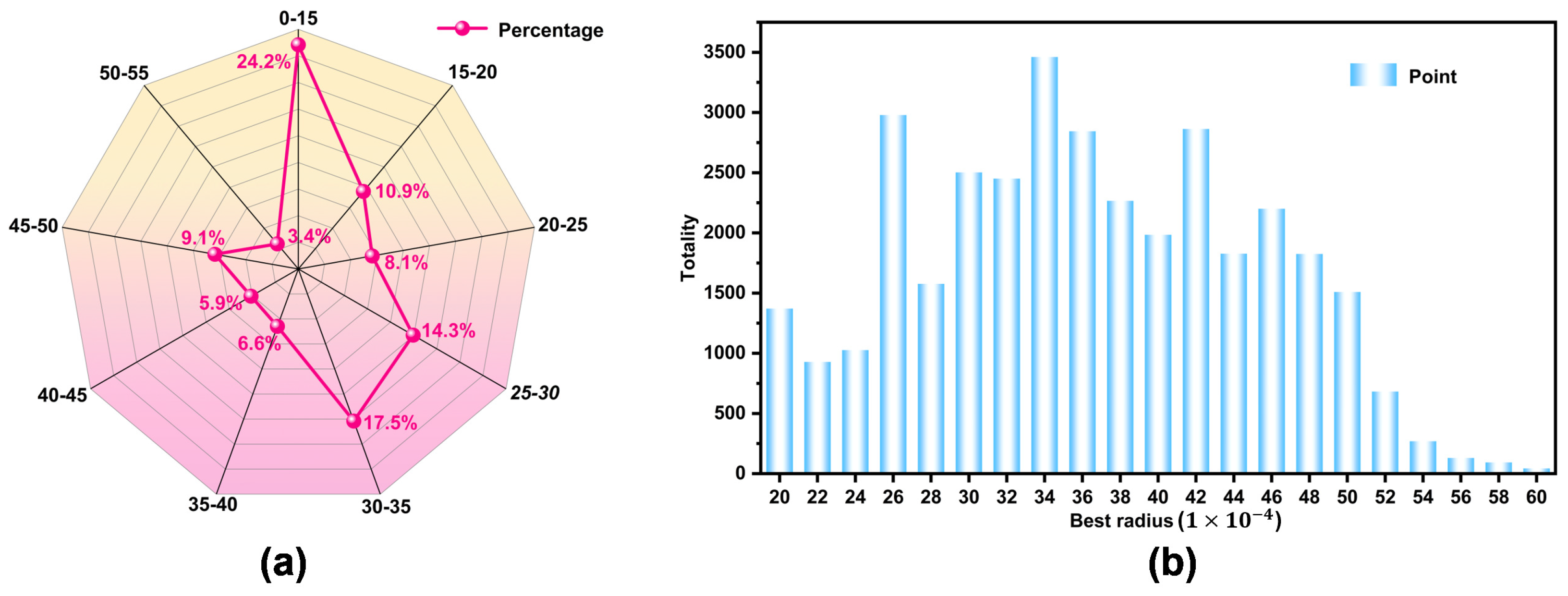
3.4. Adaptive Neighborhood Selection
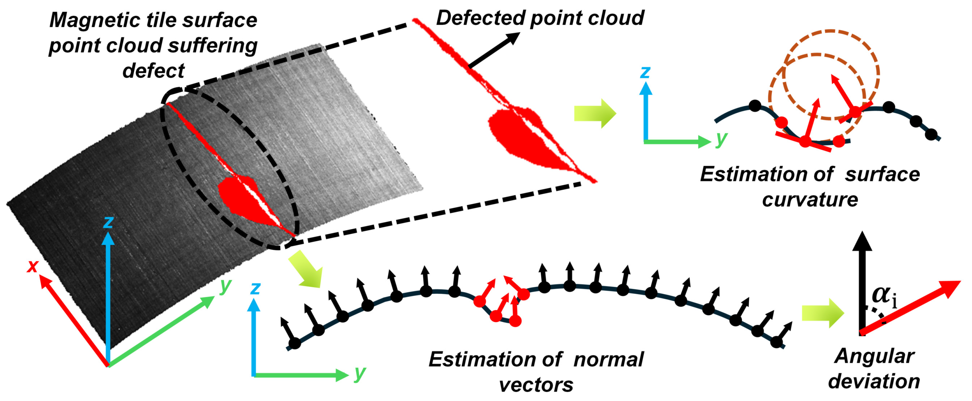
3.5. Normals and Curvature Estimation
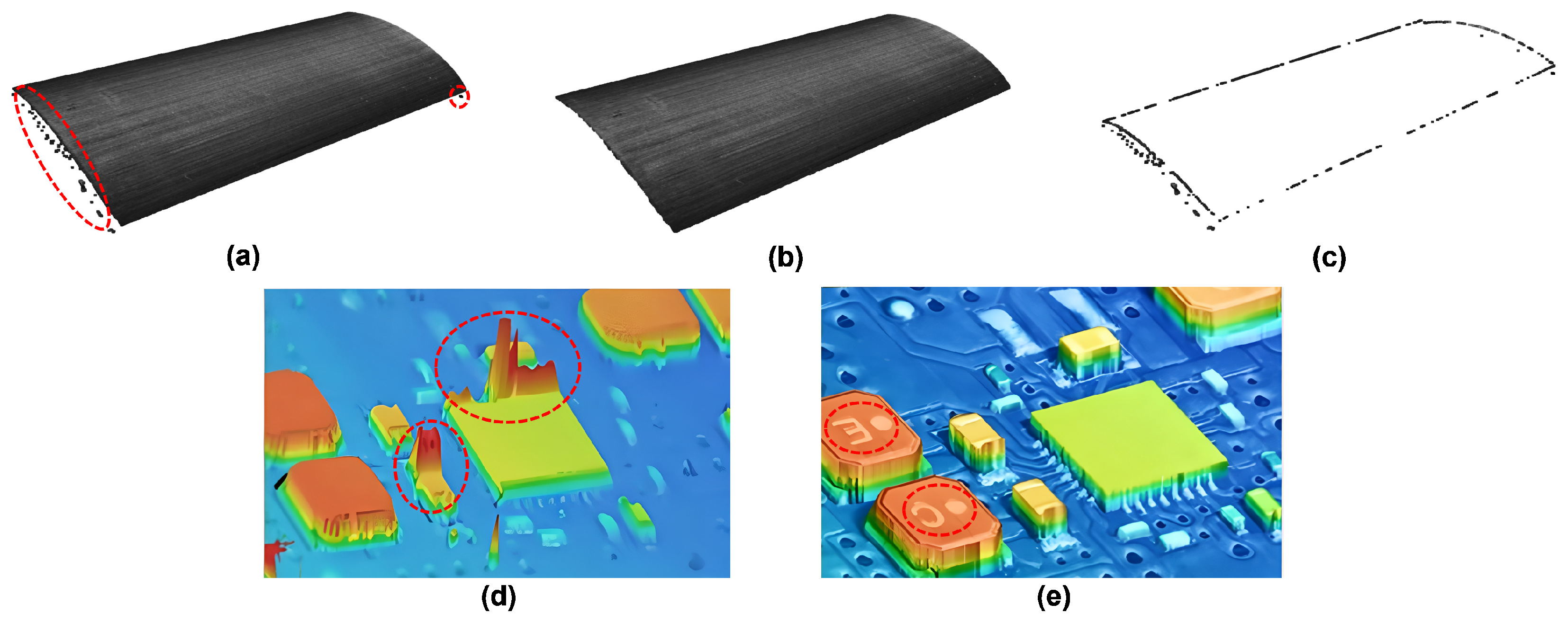
3.6. Contour Fitting Based on Single-Frame and Multi-Frame Point Clouds
3.7. Surface Defect Detection
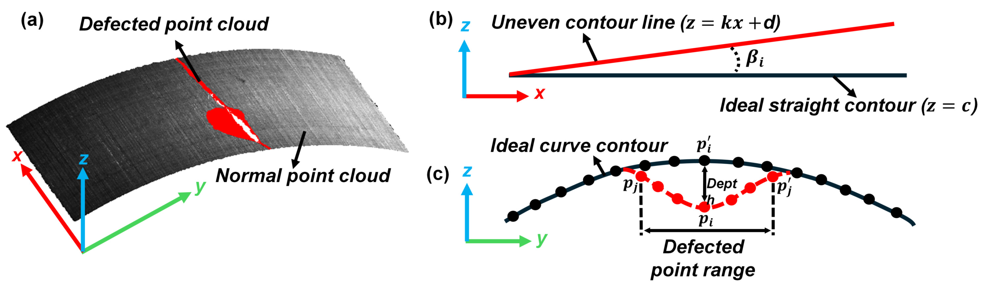
3.8. Quantitative Evaluation of Defect Severity
4. Experimental Results and Discussion
4.1. Feasibility of Normal Vectors and Curvature
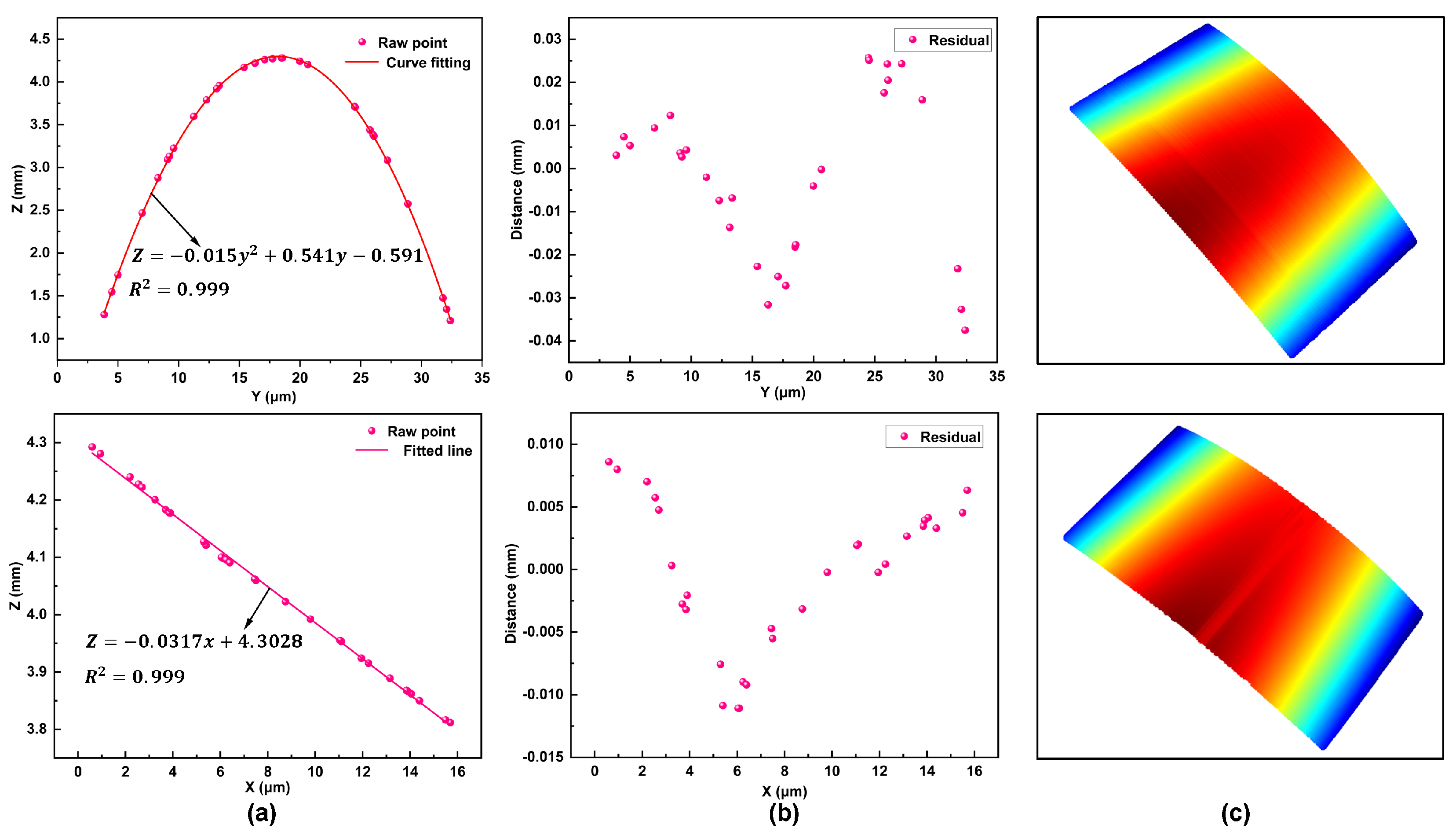
4.2. Validity of the Fitting
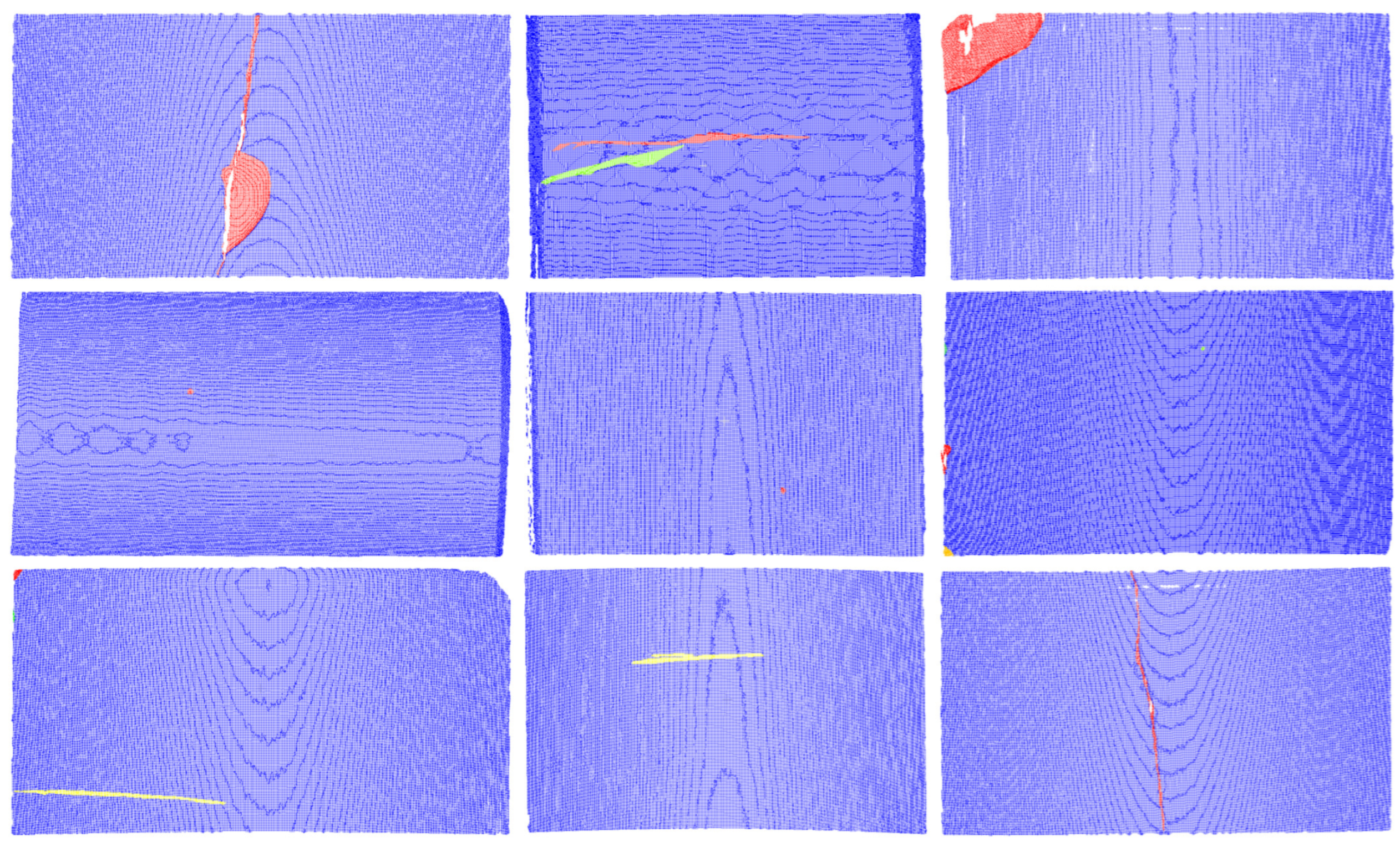
4.3. Case Study of Defect Detection
4.4. Comparison of Defect Sizes
4.5. Future Work
5. Conclusions
Author Contributions
Funding
Institutional Review Board Statement
Informed Consent Statement
Data Availability Statement
Conflicts of Interest
Appendix A
- (1)
- Indicesi and j: The index of a pixel or a point, where i = 0, 1, 2, …, n; j = 0, 1, 2, …, n.
- (2)
- Statistical filteringk: The k nearest neighbors surrounding a given point p.: The mean Euclidean distance of the k nearest neighbors from the given point p.: The standard deviation of the Euclidean distances between the k nearest neighbors and the given point p.: A scaling factor used to adjust the stringency of filtering.
- (3)
- Bilinear interpolation: The x-coordinate of a given pixel .: The y-coordinate of a given pixel .: The luminance value of a given pixel .
- (4)
- Least-squares fittingy: The y-coordinate of a given point p.z: The z-coordinate of a given point p.x: The x-coordinate of a given point p.: The original z-coordinate value of the ith point.
- (5)
- Surface defect detection algorithm: The angular deviation between the optimal normal vector of the ith point and the average normal vector of its neighboring points.: The mean curvature of all points within the adaptive neighborhood.: The standard deviation of the curvature of all points within the adaptive neighborhood.: A scale factor used to adjust the range of curvature deviation.: The height difference between two adjacent points on the same fitted contour in the x-direction.: The value of the height difference (residual) to be estimated.: The height difference (residual) of the ith observation point.
References
- Cao, X.; Chen, B.; He, W. Unsupervised Defect Segmentation of Magnetic Tile Based on Attention Enhanced Flexible U-Net. IEEE Trans. Instrum. Meas. 2022, 71, 1–10. [Google Scholar] [CrossRef]
- Ben Gharsallah, M.; Ben Braiek, E. Defect identification in magnetic tile images using an improved nonlinear diffusion method. Trans. Inst. Meas. Control 2021, 43, 2413–2424. [Google Scholar] [CrossRef]
- Jiang, C.; Zhang, X.; Xu, B.; Zheng, Q.; Li, Z.; Zhang, L.; Zhang, D. MT-U2Net: Lightweight detection network for high-precision magnetic tile surface defect localization. Mater. Today Commun. 2024, 41, 110480. [Google Scholar] [CrossRef]
- Li, Z.; Song, S.; Liu, X.; Suo, H.; Liu, W.; Song, Y. A zero-shot quantitative evaluation model for subsurface defects size based on ultrasonic nondestructive testing. Measurement 2025, 241, 115738. [Google Scholar] [CrossRef]
- Liang, C.; Wang, G.; Ma, H.; Xiao, Q.; Yu, X. A composite testing method of homologous magnetic flux leakage and motion-induced eddy current for inner and outer defects. Measurement 2025, 240, 115544. [Google Scholar] [CrossRef]
- Wu, Q.; Dong, K.; Qin, X.; Hu, Z.; Xiong, X. Magnetic particle inspection: Status, advances, and challenges—Demands for automatic non-destructive testing. NDT E Int. 2024, 143, 103030. [Google Scholar] [CrossRef]
- Vera, J.; Caballero, L.; Taboada, M. Reliability of Dye Penetrant Inspection Method to Detect Weld Discontinuities. Russ. J. Nondestr. Test. 2024, 60, 85–95. [Google Scholar] [CrossRef]
- Segovia Ramírez, I.; García Márquez, F.P.; Papaelias, M. Review on additive manufacturing and non-destructive testing. J. Manuf. Syst. 2023, 66, 260–286. [Google Scholar] [CrossRef]
- Chen, L.; Yao, X.; Xu, P.; Moon, S.K.; Bi, G. Rapid surface defect identification for additive manufacturing with in-situ point cloud processing and machine learning. Virtual Phys. Prototyp. 2021, 16, 50–67. [Google Scholar] [CrossRef]
- Inês Silva, M.; Malitckii, E.; Santos, T.G.; Vilaça, P. Review of conventional and advanced non-destructive testing techniques for detection and characterization of small-scale defects. Prog. Mater. Sci. 2023, 138, 101155. [Google Scholar] [CrossRef]
- Tang, S.; Wang, G.; Zhang, H. In situ 3D monitoring and control of geometric signatures in wire and arc additive manufacturing. Surf. Topogr-Metrol. 2019, 7, 025013. [Google Scholar] [CrossRef]
- Sohail, S.S.; Himeur, Y.; Kheddar, H.; Amira, A.; Fadli, F.; Atalla, S.; Copiaco, A.; Mansoor, W. Advancing 3D point cloud understanding through deep transfer learning: A comprehensive survey. Inform. Fusion 2025, 113, 102601. [Google Scholar] [CrossRef]
- Yang, C.; Liu, P.; Yin, G.; Jiang, H.; Li, X. Defect detection in magnetic tile images based on stationary wavelet transform. NDT E Int. 2016, 83, 78–87. [Google Scholar] [CrossRef]
- Xie, L.; Lin, L.; Yin, M.; Meng, L.; Yin, G. A novel surface defect inspection algorithm for magnetic tile. Appl. Surf. Sci. 2016, 375, 118–126. [Google Scholar] [CrossRef]
- Li, D.; Niu, Z.; Peng, D. Magnetic Tile Surface Defect Detection Based on Texture Feature Clustering. J. Shanghai Jiaotong Univ. Sci. 2019, 24, 663–670. [Google Scholar] [CrossRef]
- Wan, B.; Zhou, X.; Zheng, B.; Yin, H.; Zhu, Z.; Wang, H.; Sun, Y.; Zhang, J.; Yan, C. LFRNet: Localizing, Focus, and Refinement Network for Salient Object Detection of Surface Defects. IEEE Trans. Instrum. Meas. 2023, 72, 1–12. [Google Scholar] [CrossRef]
- Yang, B.; Liu, Z.; Duan, G.; Tan, J. Residual shape adaptive dense-nested Unet: Redesign the long lateral skip connections for metal surface tiny defect inspection. Pattern Recogn. 2024, 147, 110073. [Google Scholar] [CrossRef]
- Luo, F.; Cui, Y.; Liao, Y. MVRA-UNet: Multi-View Residual Attention U-Net for Precise Defect Segmentation on Magnetic Tile Surface. IEEE Access 2023, 11, 135212–135221. [Google Scholar] [CrossRef]
- Zhong, Z.; Wang, H.; Xiang, D. Small Defect Detection Based on Local Structure Similarity for Magnetic Tile Surface. Electronics 2023, 12, 185. [Google Scholar] [CrossRef]
- Huang, Y.; Huang, Z.; Jin, T. DEU-Net: A Multi-Scale Fusion Staged Network for Magnetic Tile Defect Detection. Appl. Sci. 2024, 14, 4724. [Google Scholar] [CrossRef]
- Huang, Y.; Qiu, C.; Yuan, K. Surface defect saliency of magnetic tile. Vis. Comput. 2020, 36, 85–96. [Google Scholar] [CrossRef]
- Yuan, H.; Peng, J. LCSeg-Net: A low-contrast images semantic segmentation model with structural and frequency spectrum information. Pattern Recogn. 2024, 151, 110428. [Google Scholar] [CrossRef]
- Zhu, Y.; Xie, L.; Yin, M.; Yin, G. Convolution With Rotation Invariance for Online Detection of Tiny Defects on Magnetic Tile Surface. IEEE Trans. Instrum. Meas. 2023, 72, 1–12. [Google Scholar] [CrossRef]
- Liu, T.; Ye, W. A semi-supervised learning method for surface defect classification of magnetic tiles. Mach. Vision Appl. 2022, 33, 35. [Google Scholar] [CrossRef]
- Kang, D.; Lai, J.; Han, Y. Accurate detection of surface defects by decomposing unreliable tasks under boundary guidance. Expert. Syst. Appl. 2024, 244, 122977. [Google Scholar] [CrossRef]
- Dekhovich, A.; Bessa, M.A. Continual learning for surface defect segmentation by subnetwork creation and selection. J. Intell. Manuf. 2024, 1–15. [Google Scholar] [CrossRef]
- Hou, W.; Jing, H. RC-YOLOv5s: For tile surface defect detection. Vis. Comput. 2024, 40, 459–470. [Google Scholar] [CrossRef]
- Gong, Y.; Wang, X.; Zhou, C.; Ge, M.; Liu, C.; Zhang, X. Human–machine knowledge hybrid augmentation method for surface defect detection based few-data learning. J. Intell. Manuf. 2024, 36, 1723–1742. [Google Scholar] [CrossRef]
- Yu, R.; Guo, B. Dynamic Reasoning Network for Image-Level Supervised Segmentation on Metal Surface Defect. IEEE Trans. Instrum. Meas. 2024, 73, 1–10. [Google Scholar] [CrossRef]
- Li, J.; Wang, K.; He, M.; Ke, L.; Wang, H. Attention-based convolution neural network for magnetic tile surface defect classification and detection. Appl. Soft. Comput. 2024, 159, 111631. [Google Scholar] [CrossRef]
- Zhou, X.; Zhou, S.; Zhang, Y.; Ren, Z.; Jiang, Z.; Luo, H. GDALR: Global Dual Attention and Local Representations in transformer for surface defect detection. Measurement 2024, 229, 114398. [Google Scholar] [CrossRef]
- Lv, C.; Zhang, E.; Qi, G.; Li, F.; Huo, J. A lightweight parallel attention residual network for tile defect recognition. Sci. Rep. 2024, 14, 21872. [Google Scholar] [CrossRef] [PubMed]
- Hu, C.; Liao, H.; Zhou, T.; Zhu, A.; Xu, C. Online recognition of magnetic tile defects based on UPM-DenseNet. Mater. Today Commun. 2022, 30, 103105. [Google Scholar] [CrossRef]
- Liu, T.; Cao, G.Z.; He, Z.; Xie, S. RoIA: Region of Interest Attention Network for Surface Defect Detection. IEEE Trans. Semiconduct. Manuf. 2023, 36, 159–169. [Google Scholar] [CrossRef]
- Li, R.; Jin, M.; Paquit, V.C. Geometrical defect detection for additive manufacturing with machine learning models. Mater. Des. 2021, 206, 109726. [Google Scholar] [CrossRef]
- Momtaz Dargahi, M.; Khaloo, A.; Lattanzi, D. Color-space analytics for damage detection in 3D point clouds. Struct. Infrastruct. Eng. 2022, 18, 775–788. [Google Scholar] [CrossRef]
- Xiong, Z.; Li, Q.; Mao, Q.; Zou, Q. A 3D Laser Profiling System for Rail Surface Defect Detection. Sensors 2017, 17, 1791. [Google Scholar] [CrossRef]
- He, Y.; Ma, W.; Li, Y.; Hao, C.; Wang, Y.; Wang, Y. An Octree-Based Two-Step Method of Surface Defects Detection for Remanufacture. Int. J. Precis. Eng. Manuf.-Green Technol. 2023, 10, 311–326. [Google Scholar] [CrossRef]
- Zhao, X.; Li, Q.; Xiao, M.; He, Z. Defect detection of 3D printing surface based on geometric local domain features. Int. J. Adv. Manuf. Technol. 2023, 125, 183–194. [Google Scholar] [CrossRef]
- Jovančević, I.; Pham, H.-H.; Orteu, J.-J.; Gilblas, R.; Harvent, J.; Maurice, X.; Brèthes, L. 3D Point Cloud Analysis for Detection and Characterization of Defects on Airplane Exterior Surface. J. Nondestruct. Eval. 2017, 36, 74. [Google Scholar] [CrossRef]
- Huang, D.; Du, S.; Li, G.; Zhao, C.; Deng, Y. Detection and monitoring of defects on three-dimensional curved surfaces based on high-density point cloud data. Precis. Eng. 2018, 53, 79–95. [Google Scholar] [CrossRef]
- Zhang, W.; Zhou, F.; Liu, Y.; Sun, P.; Chen, Y.; Wang, L. Object defect detection based on data fusion of a 3D point cloud and 2D image. Meas. Sci. Technol. 2023, 34, 025002. [Google Scholar] [CrossRef]
- Lee, E.T.; Fan, Z.; Sencer, B. A new approach to detect surface defects from 3D point cloud data with surface normal Gabor filter (SNGF). J. Manuf. Process. 2023, 92, 196–205. [Google Scholar] [CrossRef]
- Xu, Z.; Lin, Y.; Chen, D.; Yuan, M.; Zhu, Y.; Ai, Z.; Yuan, Y. Wood broken defect detection with laser profilometer based on Bi-LSTM network. Expert. Syst. Appl. 2024, 242, 122789. [Google Scholar] [CrossRef]
- Li, R.; Jin, M.; Pei, Z.; Wang, D. Geometrical defect detection on additive manufacturing parts with curvature feature and machine learning. Int. J. Adv. Manuf. Technol. 2022, 120, 3719–3729. [Google Scholar] [CrossRef]
- Makuch, M.; Gawronek, P. 3D Point Cloud Analysis for Damage Detection on Hyperboloid Cooling Tower Shells. Remote Sens. 2020, 12, 1542. [Google Scholar] [CrossRef]
- Tang, Y.; Wang, Q.; Wang, H.; Li, J.; Ke, Y. A novel 3D laser scanning defect detection and measurement approach for automated fibre placement. Meas. Sci. Technol. 2021, 32, 075201. [Google Scholar] [CrossRef]
- Cao, X.; Xie, W.; Ahmed, S.M.; Li, C.R. Defect detection method for rail surface based on line-structured light. Measurement 2020, 159, 107771. [Google Scholar] [CrossRef]
- Liu, M.; Bai, X.; Xi, S.; Dong, H.; Li, R.; Zhang, H.; Zhou, X. Detection and quantitative evaluation of surface defects in wire and arc additive manufacturing based on 3D point cloud. Virtual Phys. Prototyp. 2024, 19, e2294336. [Google Scholar] [CrossRef]
- Zheng, Q.; Zou, B.; Chen, W.; Wang, X.; Quan, T.; Ma, X. Study on the 3D-printed surface defect detection based on multi-row cyclic scanning method. Measurement 2023, 223, 113823. [Google Scholar] [CrossRef]
- Liu, X.; Wu, L.; Guo, X.; Andriukaitis, D.; Królczyk, G.; Li, Z. A novel approach for surface defect detection of lithium battery based on improved K-nearest neighbor and Euclidean clustering segmentation. Int. J. Adv. Manuf. Technol. 2023, 127, 971–985. [Google Scholar] [CrossRef]
- Puliti, M.; Montaggioli, G.; Sabato, A. Automated subsurface defects’ detection using point cloud reconstruction from infrared images. Autom. Constr. 2021, 129, 103829. [Google Scholar] [CrossRef]
- Wang, Q.; Wang, X.; He, Q.; Huang, J.; Huang, H.; Wang, P.; Yu, T.; Zhang, M. 3D tensor-based point cloud and image fusion for robust detection and measurement of rail surface defects. Autom. Constr. 2024, 161, 105342. [Google Scholar] [CrossRef]
- Zheng, L.; Lou, H.; Xu, X.; Lu, J. Tire Defect Detection via 3D Laser Scanning Technology. Appl. Sci. 2023, 13, 11350. [Google Scholar] [CrossRef]
- Zong, Y.; Liang, J.; Wang, H.; Ren, M.; Zhang, M.; Li, W.; Lu, W.; Ye, M. An intelligent and automated 3D surface defect detection system for quantitative 3D estimation and feature classification of material surface defects. Opt. Lasers Eng. 2021, 144, 106633. [Google Scholar] [CrossRef]
- Charles, R.Q.; Su, H.; Kaichun, M.; Guibas, L.J. PointNet: Deep Learning on Point Sets for 3D Classification and Segmentation. In Proceedings of the 2017 IEEE Conference on Computer Vision and Pattern Recognition (CVPR), Honolulu, HI, USA, 21–26 July 2017; pp. 77–85. [Google Scholar] [CrossRef]
- Qi, C.R.; Yi, L.; Su, H.; Guibas, L.J. Pointnet++: Deep hierarchical feature learning on point sets in a metric space. In Proceedings of the 31th Neural Information Processing Systems (NeurIPS), Long Beach, CA, USA, 4–9 December 2017; Volume 30. [Google Scholar] [CrossRef]
- Liu, Z.; Lin, Y.; Cao, Y.; Hu, H.; Wei, Y.; Zhang, Z.; Lin, S.; Guo, B. Swin Transformer: Hierarchical Vision Transformer using Shifted Windows. In Proceedings of the 2021 IEEE/CVF International Conference on Computer Vision (ICCV), Montreal, QC, Canada, 10–17 October 2021; pp. 9992–10002. [Google Scholar] [CrossRef]
- Wu, W.; Qi, Z.; Fuxin, L. PointConv: Deep Convolutional Networks on 3D Point Clouds. In Proceedings of the 2019 IEEE/CVF Conference on Computer Vision and Pattern Recognition (CVPR), Long Beach, CA, USA, 15–20 June 2019; pp. 9613–9622. [Google Scholar] [CrossRef]
- Ma, X.; Qin, C.; You, H.; Ran, H.; Fu, Y. Rethinking network design and local geometry in point cloud: A simple residual MLP framework. In Proceedings of the 10th International Conference on Learning Representations, Virtual, 25–29 April 2022; p. 07123. [Google Scholar] [CrossRef]
- Qian, G.; Li, Y.; Peng, H.; Mai, J.; Hammoud, H.; Elhoseiny, M.; Ghanem, B. PointNeXt: Revisiting PointNet++ with Improved Training and Scaling Strategies. In Proceedings of the 36th Neural Information Processing Systems (NeurIPS), New Orleans, LA, USA, 28 November 2022; Volume 35, pp. 23192–23204. [Google Scholar] [CrossRef]
- Zhou, Y.; Ji, A.; Zhang, L. Sewer defect detection from 3D point clouds using a transformer-based deep learning model. Autom. Constr. 2022, 136, 104163. [Google Scholar] [CrossRef]
- Wang, N.; Ma, D.; Du, X.; Li, B.; Di, D.; Pang, G.; Duan, Y. An automatic defect classification and segmentation method on three-dimensional point clouds for sewer pipes. Tunn. Undergr. Space Technol. 2024, 143, 105480. [Google Scholar] [CrossRef]
- Hu, Q.; Hao, K.; Wei, B.; Li, H. An efficient solder joint defects method for 3D point clouds with double-flow region attention network. Adv. Eng. Inform. 2022, 52, 101608. [Google Scholar] [CrossRef]
- García Peña, D.; García Pérez, D.; Díaz Blanco, I.; Juárez, J.M. Exploring deep fully convolutional neural networks for surface defect detection in complex geometries. Int. J. Adv. Manuf. Technol. 2024, 134, 97–111. [Google Scholar] [CrossRef]
- Pan, Y.; Yang, F.; Peng, W.; Liu, Q.; Zhang, C. Improved PointNet with accuracy and efficiency trade-off for online detection of defects in laser processing. Opt. Lasers Eng. 2025, 184, 108610. [Google Scholar] [CrossRef]
- Munakata, Y.; Pfaffly, J. Hebbian learning and development. Dev. sci. 2004, 7, 141–148. [Google Scholar] [CrossRef]
- Suchocki, C.; Błaszczak-Bąk, W.; Janicka, J.; Dumalski, A. Detection of defects in building walls using modified OptD method for down-sampling of point clouds. Build. Res. Inf. 2021, 49, 197–215. [Google Scholar] [CrossRef]
- Rusu, R.B.; Marton, Z.C.; Blodow, N.; Dolha, M.; Beetz, M. Towards 3D Point cloud based object maps for household environments. Robot. Auton. Syst. 2008, 56, 927–941. [Google Scholar] [CrossRef]
- Mancini, F.; Castagnetti, C.; Rossi, P.; Dubbini, M.; Fazio, N.L.; Perrotti, M.; Lollino, P. An Integrated Procedure to Assess the Stability of Coastal Rocky Cliffs: From UAV Close-Range Photogrammetry to Geomechanical Finite Element Modeling. Remote Sens. 2017, 9, 197–215. [Google Scholar] [CrossRef]
- Lin, Y.J.; Benziger, R.R.; Habib, A. Planar-based adaptive down-sampling of point clouds. Photogramm. Eng. Remote Sens. 2016, 82, 955–966. [Google Scholar] [CrossRef]
- Maglo, A.; Lavoué, G.; Dupont, F.; Hudelot, C. 3d mesh compression: Survey, comparisons, and emerging trends. ACM Comput. Surv. 2015, 47, 1–41. [Google Scholar] [CrossRef]
- Smith, P.R. Bilinear interpolation of digital images. Ultramicroscopy 1981, 6, 201–204. [Google Scholar] [CrossRef]
- Chen, Y.; Wu, K.; Chen, X.; Tang, C.; Zhu, Q. An entropy-based uncertainty measurement approach in neighborhood systems. Inf. Sci. 2014, 279, 239–250. [Google Scholar] [CrossRef]
- Lord, W.M.; Sun, J.; Bollt, E.M. Geometric k-nearest neighbor estimation of entropy and mutual information. Chaos 2018, 28, 033114. [Google Scholar] [CrossRef]
- Mariello, A.; Battiti, R. Feature Selection Based on the Neighborhood Entropy. IEEE Trans. Neural Netw. Learn. Syst. 2018, 29, 6313–6322. [Google Scholar] [CrossRef]
- Wang, C.; Huang, Y.; Shao, M.; Hu, Q.; Chen, D. Feature Selection Based on Neighborhood Self-Information. IEEE Trans. Cybern. 2020, 50, 4031–4042. [Google Scholar] [CrossRef]
- Guldur Erkal, B.; Hajjar, J.F. Laser-based surface damage detection and quantification using predicted surface properties. Autom. Constr. 2017, 83, 285–302. [Google Scholar] [CrossRef]
- D’Agostini, G. On the use of the covariance matrix to fit correlated data. Nucl. Instrum. Methods Phys. Res. Sect. A 1994, 346, 306–311. [Google Scholar] [CrossRef]
- Klema, V.; Laub, A. The singular value decomposition: Its computation and some applications. IEEE Trans. Autom. Control 1980, 25, 164–176. [Google Scholar] [CrossRef]
- Lin, J. Divergence measures based on the Shannon entropy. IEEE Trans. Inf. Theory 1991, 37, 145–151. [Google Scholar] [CrossRef]
- Levie, R.d. Curve Fitting with Least Squares. Crit. Rev. Anal. Chem. 2000, 30, 59–74. [Google Scholar] [CrossRef]
- Chicco, D.; Warrens, M.J.; Jurman, G. The coefficient of determination R-squared is more informative than SMAPE, MAE, MAPE, MSE and RMSE in regression analysis evaluation. Peerj Comput. Sci. 2021, 7, e623. [Google Scholar] [CrossRef]
- Kristan, M.; Leonardis, A.; Skočaj, D. Multivariate online kernel density estimation with Gaussian kernels. Pattern Recong. 2011, 44, 2630–2642. [Google Scholar] [CrossRef]
- Andersson, B.; von Davier, A.A. Improving the bandwidth selection in kernel equating. J. Educ. Meas. 2014, 51, 223–238. [Google Scholar] [CrossRef]
- Mahesh Kumar, K.; Rama Mohan Reddy, A. A fast DBSCAN clustering algorithm by accelerating neighbor searching using Groups method. Pattern Recogn. 2016, 58, 39–48. [Google Scholar] [CrossRef]
- Groth, D.; Hartmann, S.; Klie, S.; Selbig, J. Principal Components Analysis. Comput. Toxicol. 2013, 2, 527–547. [Google Scholar] [CrossRef]
- Goutte, C.; Gaussier, E. A Probabilistic Interpretation of Precision, Recall and F-Score, with Implication for Evaluation. In Advances in Information Retrieval; Springer: Berlin/Heidelberg, Germany, 2005; pp. 345–359. [Google Scholar] [CrossRef]


| Model | Scan Z Height | Scan X Length | Z-Axis Accuracy | X-Axis Accuracy | Single Line Points |
|---|---|---|---|---|---|
| KEYENCE LJ-X8060 | 64 ± 7.3 mm | 16 mm | 0.4 m | 0.5 m | 3200 |
| Method Name | Parameter Details |
|---|---|
| Statistical filtering | , |
| Adaptive neighborhood selection | , , , k: adaptive |
| Normal vector deviation | , k: adaptive |
| Curvature deviation | , k: adaptive |
| Coarse detection and fine extraction | Corresponding to the top 5th percentile and top 2nd percentile, respectively. |
| DBSCAN clustering | , |
| Method Name | Severe Defect | Tiny Defect | Severe Scratch | Minor Scratch | ||||||||
|---|---|---|---|---|---|---|---|---|---|---|---|---|
| Pre | Rec | F1 | Pre | Rec | F1 | Pre | Rec | F1 | Pre | Rec | F1 | |
| Nd | 0.5417 | 0.4877 | 0.5133 | 0.3463 | 0.8496 | 0.4920 | 0.5631 | 0.5802 | 0.5715 | - | - | - |
| Cd | 0.5629 | 0.5078 | 0.5339 | 0.3688 | 0.8547 | 0.5153 | 0.5698 | 0.5992 | 0.5841 | - | - | - |
| Mf | 0.9634 | 0.9512 | 0.9573 | 0.9320 | 0.9416 | 0.9368 | 0.8857 | 0.8404 | 0.8625 | 0.3505 | 0.7297 | 0.4735 |
| Ours | 0.9528 | 0.9697 | 0.9612 | 0.9233 | 0.9588 | 0.9407 | 0.9413 | 0.9505 | 0.9454 | 0.7375 | 0.7649 | 0.7510 |
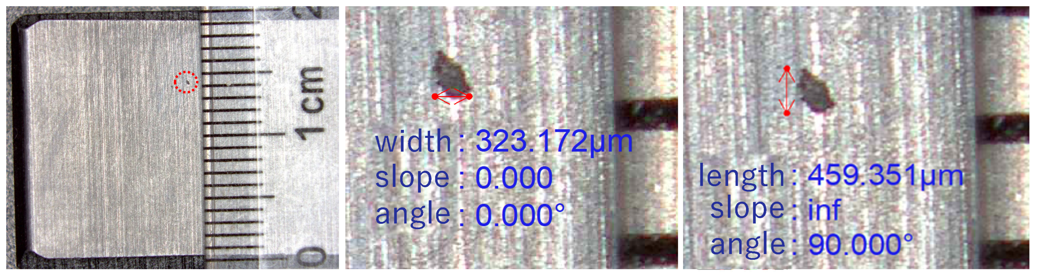
| Defect | Length (mm) | Error (%) | Width (mm) | Error (%) | Depth (mm) | Error (%) | |||
|---|---|---|---|---|---|---|---|---|---|
| R | M | R | M | R | M | ||||
| 1 | 16.160 | 15.62 | 3.34 | 3.470 | 3.351 | 3.43 | 0.483 | 0.472 | 2.28 |
| 2 | 0.527 | 0.549 | 4.17 | 0.235 | 0.247 | 5.11 | 0.031 | 0.042 | 3.55 |
| 3 | 0.360 | 0.372 | 3.33 | 0.115 | 0.183 | 5.91 | 0.082 | 0.077 | 6.10 |
| 4 | 0.615 | 0.638 | 3.74 | 0.291 | 0.304 | 4.47 | 0.052 | 0.055 | 5.77 |
| 5 | 9.682 | 9.419 | 2.72 | 0.478 | 0.459 | 3.97 | 0.038 | 0.041 | 7.89 |
| 6 | 7.080 | 7.254 | 2.46 | 0.365 | 0.377 | 3.29 | - | 0.013 | - |
| 7 | 14.845 | 14.215 | 4.24 | 0.430 | 0.407 | 5.35 | - | 0.011 | - |
| Average Error | - | - | 3.43 | - | - | 4.50 | - | - | 5.12 |
Disclaimer/Publisher’s Note: The statements, opinions and data contained in all publications are solely those of the individual author(s) and contributor(s) and not of MDPI and/or the editor(s). MDPI and/or the editor(s) disclaim responsibility for any injury to people or property resulting from any ideas, methods, instructions or products referred to in the content. |
© 2025 by the authors. Licensee MDPI, Basel, Switzerland. This article is an open access article distributed under the terms and conditions of the Creative Commons Attribution (CC BY) license (https://creativecommons.org/licenses/by/4.0/).
Share and Cite
Huang, J.; Huang, Q.; Jiang, W.; Sun, F. Entropy-Driven Adaptive Neighborhood Selection and Fitting for Sub-Millimeter Defect Detection and Quantitative Evaluation in Magnetic Tiles. Appl. Sci. 2025, 15, 3518. https://doi.org/10.3390/app15073518
Huang J, Huang Q, Jiang W, Sun F. Entropy-Driven Adaptive Neighborhood Selection and Fitting for Sub-Millimeter Defect Detection and Quantitative Evaluation in Magnetic Tiles. Applied Sciences. 2025; 15(7):3518. https://doi.org/10.3390/app15073518
Chicago/Turabian StyleHuang, Jiaxiong, Qinyuan Huang, Wengziyang Jiang, and Fei Sun. 2025. "Entropy-Driven Adaptive Neighborhood Selection and Fitting for Sub-Millimeter Defect Detection and Quantitative Evaluation in Magnetic Tiles" Applied Sciences 15, no. 7: 3518. https://doi.org/10.3390/app15073518
APA StyleHuang, J., Huang, Q., Jiang, W., & Sun, F. (2025). Entropy-Driven Adaptive Neighborhood Selection and Fitting for Sub-Millimeter Defect Detection and Quantitative Evaluation in Magnetic Tiles. Applied Sciences, 15(7), 3518. https://doi.org/10.3390/app15073518