Assessing Spatiotemporal LST Variations in Urban Landscapes Using Diurnal UAV Thermography

Abstract

This study investigates the spatiotemporal dynamics of land surface temperature (LST) across five distinct land use/land cover (LULC) classes through high-resolution unmanned aerial vehicle (UAV) thermal remote sensing. Thermal orthomosaics were systematically captured at four diurnal periods (morning, afternoon, evening, and midnight) over an urban university campus environment. Using stratified random sampling in each class with spatial controls to minimize autocorrelation, we quantified thermal signatures across bare soil, buildings, grassland, paved roads, and water bodies. Statistical analyses incorporating outlier management via the Interquartile Range (IQR) method, spatial autocorrelation assessment using Moran’s I, correlation testing, and Geographically Weighted Regression (GWR) revealed substantial thermal variability across LULC classes, with temperature differentials of up to 17.7 °C between grassland (20.57 ± 5.13 °C) and water bodies (7.10 ± 1.25 °C) during afternoon periods. The Moran’s I analysis indicated notable spatial dependence in land surface temperature, justifying the use of GWR to model these spatial patterns. Impervious surfaces demonstrated pronounced heat retention capabilities, with paved roads maintaining elevated temperatures into evening (13.18 ± 3.49 °C) and midnight (2.25 ± 1.51 °C) periods despite ambient cooling. Water bodies exhibited exceptional thermal stability (SD range: 0.79–2.85 °C across all periods), while grasslands showed efficient nocturnal cooling (ΔT = 23.02 °C from afternoon to midnight). GWR models identified spatially heterogeneous relationships between LST patterns and LULC distribution, with water bodies exerting the strongest localized cooling influence ($R^2$≈ 0.62–0.68 during morning/evening periods). The findings demonstrate that surface material properties significantly modulate diurnal heat flux dynamics, with human-made surfaces contributing to prolonged thermal loading. This research advances urban microclimate monitoring methodologies by integrating high-resolution UAV thermal imagery with robust statistical frameworks, providing empirically-grounded insights for climate-adaptive urban planning and heat mitigation strategies. Future work should incorporate multi-seasonal observations, in situ validation instrumentation, and integration with human thermal comfort indices.

1. Introduction

Understanding land surface temperature (LST) variations is critical for analyzing thermal dynamics in urban and natural environments, particularly in the context of climate change and urban planning. LST influences energy balance, urban heat island effects, and local climate resilience, making its accurate assessment essential for sustainable development and environmental management. Local climate resilience refers to the capacity of urban and natural environments to withstand, adapt to, and recover from climate-related stresses while maintaining essential functions and services. In the context of thermal dynamics, it encompasses the ability of different landscapes to moderate temperature extremes and mitigate heat-related impacts through their surface properties and cooling mechanisms [1]. This concept is increasingly crucial as cities face growing challenges from urban heat islands, extreme heat events, and changing precipitation patterns that directly impact human health, energy consumption, and ecosystem functioning [2,3]. The increasing urbanization and alteration of land cover types significantly affect surface heat retention, leading to localized temperature variations that influence microclimate conditions and energy balance [4]. Traditional satellite-based remote sensing methods, such as Landsat (16-day revisit cycle) or MODIS thermal infrared sensors (with up to four observations per day combining Terra and Aqua platforms), have been widely used to assess LST; however, these approaches are often limited by their low spatial resolution (100 m for MODIS thermal bands, 30–100 m for Landsat) and constrained temporal flexibility for capturing complete diurnal cycles, which restrict their ability to detect fine-scale temperature variations and rapid thermal transitions within urban environments [5]. As an alternative, unmanned aerial vehicles (UAVs) equipped with thermal infrared cameras provide high-resolution, on-demand thermal data collection at user-defined intervals throughout the day, allowing for more detailed temporal and spatial monitoring of temperature dynamics across different land cover types [6]. The high temporal flexibility and spatial resolution of UAV-based thermal imaging directly enables this study’s core methodological approach. While satellite platforms are limited to fixed overpass times and coarser resolutions (typically 30–100 m for Landsat/MODIS), our UAV deployment captures critical diurnal transitions (morning, afternoon, evening, and midnight) at centimeter-scale resolution. This capability is essential for detecting fine-scale thermal variations across our five target LULC classes and capturing the complete diurnal cycle of heat absorption and dissipation, which would be impossible using traditional satellite methods. The temporal granularity afforded by UAV platforms is particularly crucial for quantifying nocturnal cooling rates and heat retention differences among urban materials—key processes in understanding urban microclimate dynamics that satellite-based approaches cannot adequately resolve. UAV-based thermal imaging has been particularly effective in studying small-scale surface temperature variations, detecting urban heat island effects, and evaluating surface heat retention across various land uses [7].

Different land cover types exhibit distinct thermal responses due to their surface material properties. Impervious surfaces, such as asphalt and concrete, typically absorb and retain more heat than permeable surfaces like grass or water bodies, leading to significant temperature differences during the day [8]. UAV-based studies have documented temperature variations of up to 25 °C between urban and vegetated surfaces, highlighting the importance of land cover in modulating heat accumulation [9]. Moreover, natural surfaces, such as grasslands and water bodies, exhibit lower thermal fluctuations due to evapotranspiration and higher specific heat capacity, which contribute to effective heat dissipation [10]. Despite these findings, there remains a research gap in understanding the precise temporal thermal behavior of different land cover types, particularly under varying atmospheric conditions such as humidity, wind speed, and cloud cover, which influence heat retention and dissipation patterns.

Temporal monitoring of LST at different times of the day is essential for capturing diurnal thermal dynamics and understanding how surfaces respond to solar radiation. Studies have shown that asphalt surfaces can experience temperature increases of up to 30 °C from morning to afternoon, while vegetated areas remain more thermally stable due to their transpiration-driven cooling effects [11]. Water bodies, on the other hand, exhibit minimal temperature fluctuations due to their high thermal inertia, making them effective heat buffers [12]. UAV-based thermal monitoring allows researchers to capture these changes at a high temporal resolution, providing deeper insights into heat accumulation and dissipation patterns. However, challenges remain regarding the accuracy of UAV-derived LST measurements, which can be influenced by factors such as sensor calibration, surface emissivity variations, and atmospheric conditions [13]. Several studies comparing UAV-based thermal imagery with in situ infrared thermometer readings have reported root mean square errors ranging from 1.5 °C to 5.5 °C, depending on land cover and meteorological conditions [14]. The current findings demonstrate that sensor calibration and validation are a prerequisite for utilizing UAV-derived thermal data in studies demanding absolute temperature measurement.

Despite recent advancements in UAV-based thermal imaging, comprehensive studies integrating these methods with meteorological temperature records to analyze diurnal LST variations across multiple land use/land cover (LULC) types remain scarce. While previous research has largely concentrated on urban heat island assessments or agricultural applications, the high-resolution dynamics of surface temperature over the full diurnal cycle have not been thoroughly investigated—a gap that is increasingly critical given the rising frequency of extreme heat events under climate change. Addressing this need, our study investigates the diurnal thermal behavior of five distinct LULC classes—bare soil, buildings, grassland, paved roads, and water bodies—using UAV-mounted thermal cameras. Data are captured at four key periods—morning, afternoon, evening, and midnight—facilitating a time-specific assessment of LST variations. By integrating high-resolution UAV-based thermal images with robust statistical analyses, this research systematically examines the complete diurnal temperature cycle across diverse surfaces. Such an approach enhances our understanding of surface–atmosphere interactions and localized thermal anomalies while providing critical information for urban microclimate modeling, heat island mitigation strategies, and climate-adaptive urban planning.

2. Literature Review

The widespread adoption of UAVs and the integration of various sensors have significantly expanded their range of applications. A critical examination reveals important methodological patterns, technological advancements, and research gaps across diverse domains of these applications.

UAV-based thermal platforms have evolved across multiple application domains, each contributing to the methodological advancement. In agricultural contexts, Santesteban et al. [15] pioneered the high-resolution monitoring of plant water status in vineyards, while Ortiz-Sanz et al. [16] and Perich et al. [17] extended these approaches to wine cellars and crop phenotyping, respectively. These agricultural applications established fundamental approaches for surface temperature characterization. Concurrently, Nieto et al. [18] developed methodologies for evaporation studies, while Casana et al. [19] demonstrated archaeological applications, and Zheng et al. [20] applied thermal imaging to building energy assessment. This cross-disciplinary development reflects the progressive refinement of UAV thermal methodology, though most early applications focused on limited temporal sampling.

Sensor performance studies have been critical to methodological advancement. Kelly et al. [21] systematically documented internal temperature fluctuations in thermal sensors, while Acorsi et al. [22] provided comparative analysis between ground and airborne thermal measurements. These foundational studies identified key measurement challenges subsequently addressed through radiometric calibration procedures developed by Aragon et al. [23] and Henn and Peduzzi [24]. Further refinements addressed emissivity effects (Song and Park [25]) and camera angle influences (Lee et al. [26]). This methodological progression reflects increasing sophistication in addressing measurement accuracy—a critical consideration when comparing results across studies conducted in different urban environments.

The comparative assessment of urban thermal studies reveals considerable variation in spatiotemporal frameworks. Naughton and McDonald [27] documented from 3.9 to 15.8 °C LST differences across urban land covers in Milwaukee and El Paso through single-time-point monitoring. Similar methodological approaches by Soto-Estrada et al. [28] quantified tree shading effects, finding 12 °C reductions for asphalt and 5.7 °C for concrete surfaces in Medellin. These point-in-time studies provided valuable surface comparisons but lacked temporal dynamics.

Material-specific thermal behaviors have been documented across diverse urban contexts. Ahmad et al. [29] demonstrated that dark rooftops exhibited higher temperatures than light-colored alternatives, while Lee et al. [30] confirmed similar patterns in cold climate regions—suggesting consistent physical principles despite contextual variation. Son and Kim [31] documented extreme temperatures exceeding 50 °C in South Korean waterfront parks, while Yang et al. [32] integrated thermal assessments with ventilation analysis across 31 Chinese cities, finding that improved ventilation could reduce energy consumption by 6%—highlighting the importance of combining thermal assessment with urban morphology analysis.

Methodological comparisons between UAV and satellite-based approaches have established complementary strengths. Smith et al. [33] demonstrated that UAV-derived LST revealed finer-scale details than MODIS and Landsat in Chilean cities, while Xu et al. [14] used UAVs to observe how paved surfaces exhibited elevated LST and analyzed potential thermal runoff effects on nearby water bodies—capturing thermal relationships undetectable in coarser resolution data. Kim et al. [34] quantified this advantage, finding UAV-derived LST significantly outperformed Landsat in South Korean parks. Ahmad and Eisma [35] further confirmed this pattern for micro-urban heat island detection in Dallas-Fort Worth. These comparative studies consistently demonstrate the scale-dependent nature of thermal monitoring, with UAVs occupying a critical middle ground between in situ and satellite measurements.

Wang and Prigent [36] provided important context by comparing diurnal LST measurements across platforms, finding that satellite-based approaches performed adequately for homogeneous surfaces like barren lands but demonstrated reduced accuracy in vegetated areas. This finding underscores the context-dependent performance of different measurement approaches rather than suggesting universal superiority of any single platform.

A critical assessment of temporal frameworks reveals significant variation in approaches to capturing diurnal thermal patterns. Qian et al. [37] implemented three-dimensional thermal monitoring from 1.5 m to 200 m at the morning, afternoon, and night periods, providing valuable insights into vertical thermal structure but offering limited resolution of diurnal transitions. Chudnovsky et al. [8] employed ground-based radiometry complemented by UAV thermal imaging in Tel Aviv, recommending early-morning and midday measurements as critical points for capturing maximum thermal contrast—though this two-point approach necessarily simplifies complex diurnal patterns.

More comprehensive temporal frameworks have emerged in limited studies. Malbéteau et al. [38] documented approximately 20 °C daytime temperature swings in Saudi Arabian deserts compared to 12 °C in grass fields—highlighting the substantial influence of surface materials on diurnal amplitude. Wu et al. [39] demonstrated significant improvements in urban thermal characterization through integration of UAV thermal imagery with near-ground meteorological data, suggesting the importance of contextualizing thermal measurements within broader atmospheric conditions.

Although numerous studies have contributed valuable insights into UAV-based thermal imaging, most research has focused on single time points or limited daytime measurements. However, evening and nighttime measurements are crucial as they provide insights into heat retention, cooling rates, and thermal inertia effects across different land cover types, which are essential for understanding long-term microclimatic variations. Consequently, the complete diurnal cycle, particularly during evening and nighttime periods, remains under-investigated. Given that understanding these day-to-night transitions is essential for comprehending how different land cover types store and release heat, there is a clear need for a comprehensive analysis. This study aims to bridge that gap by systematically examining the full diurnal thermal behavior of various surfaces using high-resolution UAV-derived data.

3. Methods

This study investigates diurnal variations in LST across diverse LULC classes within an urban setting. The overall methodological framework encompasses systematic data acquisition, image processing and sample collection, outlier management, and a suite of advanced statistical and spatial analyses to characterize diurnal thermal behavior.

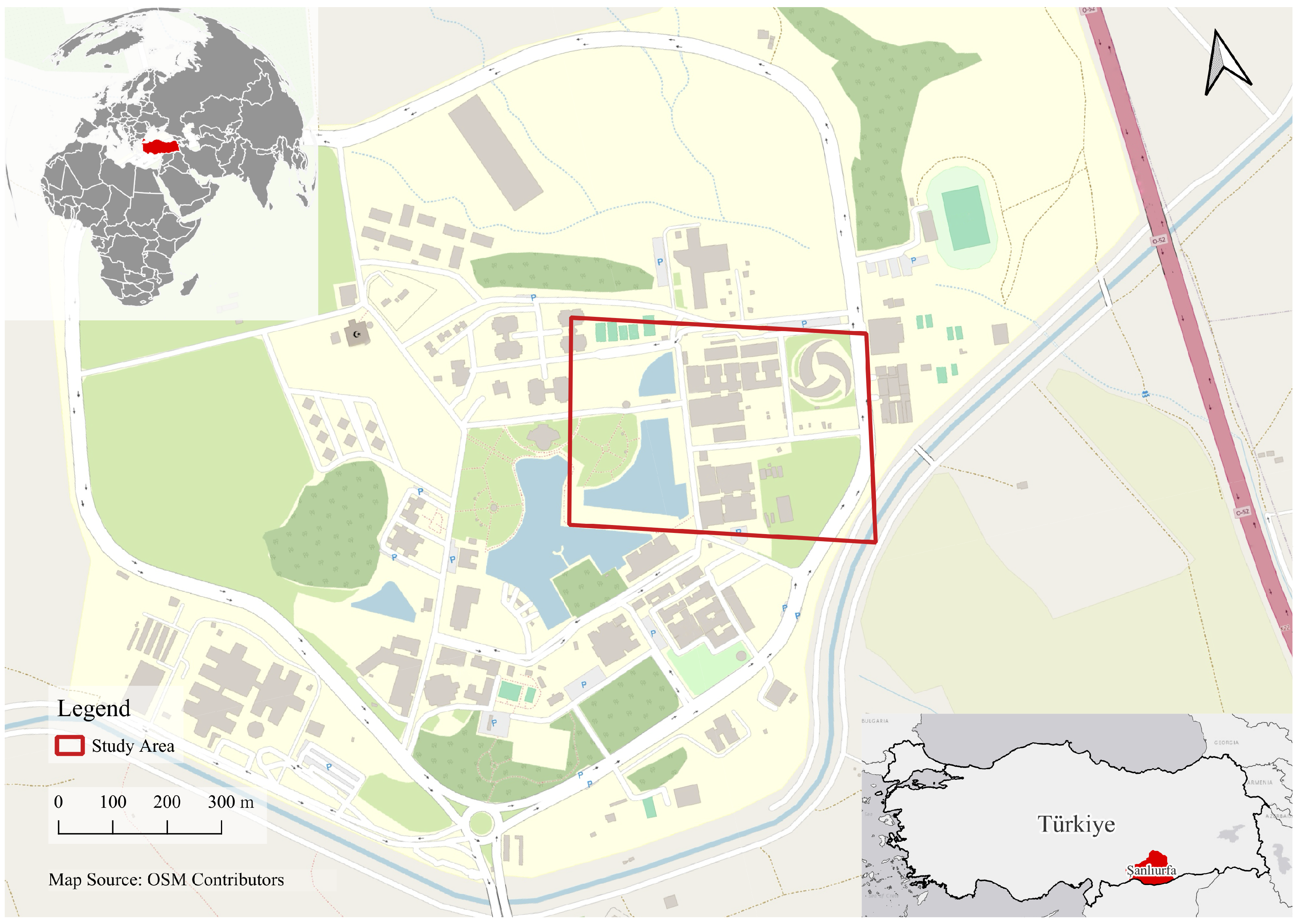
3.1. Study Area and Data Acquisition

This study was conducted on the Harran University Osmanbey Campus—a spatially diverse area featuring multiple LULC types such as lakes, bare soil, built-up areas, grasslands, and roads. Located in Şanlıurfa, the campus experiences a hot Mediterranean climate (Köppen-Geiger classification: Csa) with hot, dry summers and mild, wet winters [40,41,42]. Its well-defined, urban-like setting makes it an ideal site for investigating diurnal variations in LST across different surface types (Figure 1).

Data collection involved comprehensive thermal data acquisition using a DJI Mavic 3T Thermal quadcopter UAV (manufactured by DJI Technology Co., Ltd. headquartered in Shenzhen, China), which was selected for its advanced dual-camera payload system [43]. This system is equipped with a primary radiometric thermal camera utilizing a 640 × 512 pixel microbolometer array and a 40 mm lens with a 61° diagonal field of view. The thermal imager operates within the long-wave infrared spectral range (8–14 μm) and features a low noise equivalent temperature difference, enabling the acquisition of high-fidelity temperature measurements across a detection range from −20 °C to 150 °C. The system maintains a temperature measurement accuracy of ±2 °C or ±2% of the reading, whichever is greater. Complementing the thermal sensor, a secondary RGB camera, featuring a 4/3 CMOS sensor with a mechanical shutter, captured concurrent visual imagery at a resolution of 20 megapixels (5280 × 3956 pixels).

UAV flights were systematically conducted over the campus area in January 2025 at four distinct diurnal periods: morning (8:00–9:00), afternoon (12:00–13:00), evening (17:00–18:00), and midnight (22:00–23:00). These periods were specifically chosen to capture the key phases of diurnal thermal dynamics, from peak solar radiation to nocturnal cooling (sunrise: 7:30, sunset: 17:46). Photogrammetric UAV flights were executed following a standardized flight plan at a height of 40 m, with 80% transverse and longitudinal overlap ratios, yielding 1524 thermal aerial images per flight at a ground sample resolution of 5.66 cm/pix. Concurrent with thermal data acquisition, ambient air temperature measurements were recorded using a standard digital thermometer positioned at the UAV launch location. Temperature readings were taken at the beginning and end of each flight period (morning, afternoon, evening, and midnight) at approximately 1.5 m above ground level to provide contextual reference data for the thermal imagery analysis. It should be noted that these ambient temperature measurements were collected primarily to establish general atmospheric conditions during the data acquisition periods rather than to characterize the microclimate of specific LULC classes. A single representative temperature value was calculated for each diurnal period by averaging the recorded measurements. These ambient temperature reference points serve as important contextual data for interpreting the relative patterns in the thermal orthophotos, particularly when assessing the differential between air temperature and surface temperature across various LULC types.

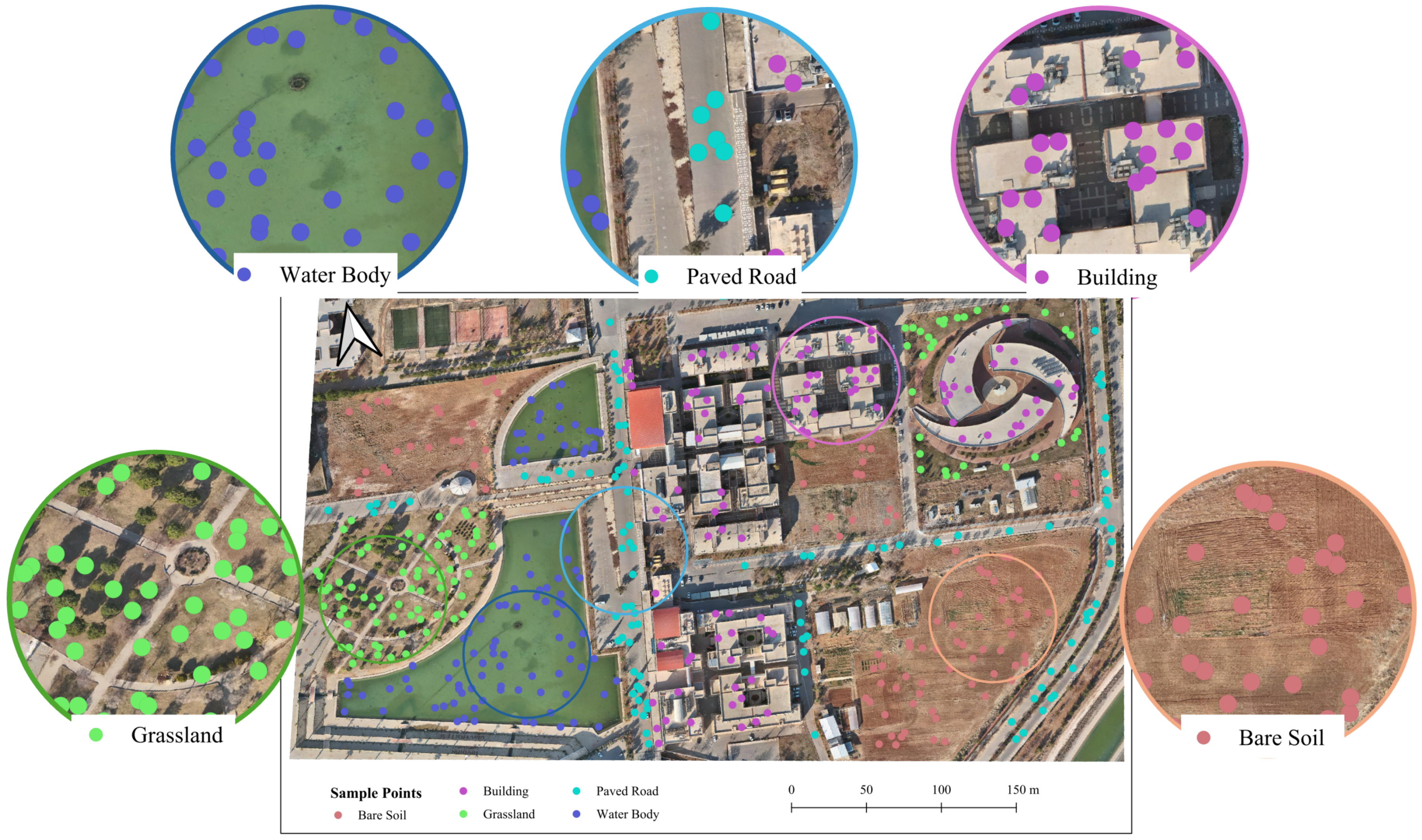
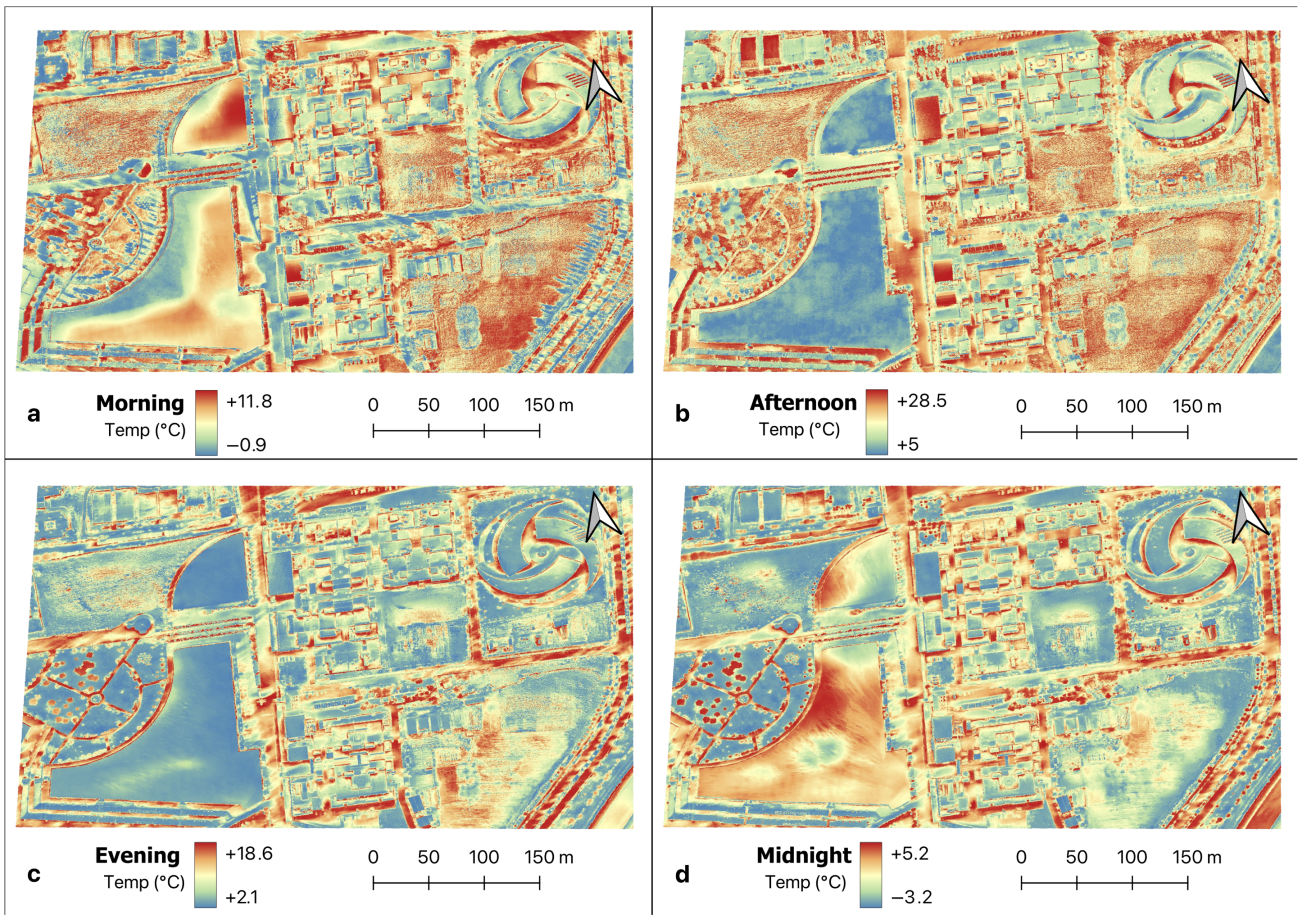
3.2. Thermal Image Processing and Sample Collection

Following the acquisition of thermal imagery during each UAV flight, a detailed photogrammetric workflow was implemented to produce high-resolution thermal orthophotos using Structure from Motion (SfM) photogrammetry. SfM is a computational technique that converts two-dimensional thermal images into geometrically corrected orthomosaics, effectively reconstructing the thermal landscape in three dimensions [44]. This process involved capturing overlapping photographs from multiple vantage points and employing specialized algorithms to detect and match keypoints across images, thereby generating a sparse point cloud. This sparse point cloud was subsequently refined into a dense point cloud through advanced image correlation methods. A Digital Elevation Model (DEM) was then constructed from the dense point cloud and integrated into the generation of the final thermal orthophotos, which serve as the foundational dataset for subsequent LST analysis [44,45].

For subsequent analysis, a stratified random sampling approach was employed within each of the identified LULC classes. To ensure spatial representativeness during stratified random sampling, we implemented distance-based controls with minimum threshold distances varying between 0.5 and 1 m based on the specific characteristics of each LULC class. This adaptive distance approach allowed for appropriate sampling density while minimizing spatial autocorrelation effects. Prior to sampling, we systematically reviewed and modified the delineation of LULC areas to exclude patches with complex geometries or insufficient size that could introduce sampling bias. This pre-processing step ensured that the final LULC classification included only well-defined, representative areas amenable to robust statistical analysis. First, regions of interest (ROIs) were delineated for each LULC category to define the spatial extents representative of their dominant surface types. Within each ROI, random sample points were generated and their locations recorded in projected coordinates for further spatial analyses. One hundred sample points were collected for each LULC class (totaling 500) to ensure statistical robustness and to accommodate potential outliers or measurement errors. During the sampling process, specific care was taken to exclude points from atypical surfaces. For instance, sample points were intentionally avoided on building materials such as air conditioners, chimneys, and metal fixtures on buildings; trees located within grassy areas; rocks present in bare soil areas; and parked vehicles on road surfaces. The spatial distribution of the sample points across the study area and within each LULC class is shown in Figure 2.

3.3. Outlier Management

Prior to statistical analysis, we implemented data filtering to ensure statistical robustness and reliable thermal pattern characterization. The initial dataset consisted of 500 sampling points, with 100 points collected for each of the five LULC classes. To mitigate the influence of statistical outliers that could potentially distort the interpretation of thermal behaviors, we applied the Interquartile Range (IQR) method to identify anomalous observations.

The IQR-based outlier detection was implemented independently for each LULC class and temporal period, identifying observations that fell outside the boundaries defined in Equation (1) by

$$[Q_1-1.5\times \mathrm{IQR},Q_3+1.5\times \mathrm{IQR}]$$

(1)

where $Q_1$ represents the first quartile, $Q_3$ represents the third quartile, and IQR = $Q_3-Q_1$.

This method defined outliers as observations that deviated significantly from the expected range, specifically those falling outside the 1.5 × IQR of the first and third quartiles for each categorized dataset and time period. Observations falling outside these thresholds were classified as outliers and subsequently removed from the dataset. By applying this statistical threshold, we ensured that extreme values, which could unduly influence analysis outcomes, were systematically identified and eliminated. This approach enhances data integrity and allows for a more accurate representation of underlying patterns while accommodating variations within different LULC classes and temporal conditions.

The IQR method was chosen because it provides a non-parametric approach to outlier detection that does not require assumptions about the underlying data distribution, making it suitable for potentially non-normal thermal data distributions [46,47].

3.4. Statistical Analysis

Following data pre-processing, statistical analyses were performed to characterize the thermal properties of each LULC type. Descriptive statistics, including the mean, median, standard deviation, minimum, and maximum LST values, were calculated for each LULC class and diurnal period to summarize the central tendency and dispersion of the data. Furthermore, frequency distributions, visualized through histograms overlaid with kernel density estimates, were generated to explore the distributional shapes, providing a foundational understanding of their thermal behavior.

3.5. Spatial Autocorrelation Analysis (Moran’s I)

To assess the potential for spatial dependence in LST data, a spatial autocorrelation analysis using Moran’s I statistic was conducted. A spatial weights matrix was constructed using a k-nearest neighbors (KNN) approach, with $k=8$, ensuring that each point was connected to its eight closest neighbors. The weights were row-standardized to account for variations in sampling density. Moran’s I is a widely used global measure of spatial autocorrelation that quantifies the degree to which values at one location are similar to values at nearby locations [48,49]. A positive Moran’s I value indicates spatial clustering, where similar values tend to be located close together, while a negative value suggests spatial dispersion, where dissimilar values are clustered. A value close to zero indicates a random spatial pattern.

Moran’s I was calculated for LST measurements for each of the four diurnal periods. This stratified approach allowed for the assessment of spatial autocorrelation across different temporal contexts to assess clustering between different LULC classes. For each calculation, the associated p-values were examined to determine the statistical significance of any observed spatial autocorrelation patterns. The rationale for employing Moran’s I was to rigorously examine the fundamental assumption of independence often required by classical statistical methods [50]. Given the stratified random sampling design within LULC classes, and the inherent spatial continuity of thermal phenomena, it was anticipated that LST values might exhibit spatial autocorrelation, particularly between LULC areas. The outcomes of this Moran’s I analysis were intended to inform the selection of subsequent spatial analysis techniques, specifically regarding the appropriateness of methods that account for spatial dependence versus those that assume spatial independence.

3.6. Geographically Weighted Regression (GWR) Analysis

Building upon the assessment of spatial autocorrelation (detailed in the previous section) and acknowledging the inherent spatial clustering introduced by our stratified sampling design across LULC classes, we implemented Geographically Weighted Regression (GWR) as our primary spatial analytical technique [51]. GWR is particularly appropriate for this dataset, as it explicitly models spatial non-stationarity, allowing regression parameters to vary continuously over geographic space. This approach enables the identification of localized relationships between proximity to specific LULC types and temperature variations while accounting for the inherent spatial dependence in thermal patterns [52].

To explore the spatial heterogeneity of temperature influences, GWR was implemented. For each temperature measurement point, Euclidean distances to the nearest instances of each LULC type were calculated using a k-d Tree nearest neighbor approach [53]. These distances were chosen as predictor variables, based on the hypothesis that the thermal properties of surrounding land cover significantly influence the land surface temperature at a given location. The GWR model was specified in Equation (2) as

$$T(u_i,v_i)={\beta }_0(u_i,v_i)+\sum _k{\beta }_k(u_i,v_i)X_k+{\epsilon }_i$$

(2)

where $T(u_i,v_i)$ represents the LST at location $(u_i,v_i)$, ${\beta }_k(u_i,v_i)$ are location-specific regression coefficients for each predictor variable $X_k$ (representing the Euclidean distance to the nearest instances of each LULC type), and ${\epsilon }_i$ is the error term.

The optimal bandwidth for the GWR model, which determines the spatial extent over which data points influence local parameter estimation, was determined using a cross-validation procedure. Specifically, the Golden Section Search method was employed to optimize the bandwidth by minimizing the cross-validation score [54], thereby ensuring the best possible local model fit. The performance of each GWR model was evaluated using $R^2$ and adjusted $R^2$ metrics, which quantified the proportion of variance in LST explained by the predictor variables at local scales, thus assessing the spatially varying influence of LULC features on surface temperatures.

4. Results

The thermal orthophotos resulting from the UAV data acquisition and photogrammetric processing are presented in Figure 3, illustrating the spatial distribution of LST across the study area during four diurnal periods. It should be noted that the results presented herein represent thermal conditions specific to January 2025 (winter season) in a semiarid climate, characterized by relatively cool ambient temperatures and minimal vegetation activity. These orthophotos reveal distinct thermal patterns across different LULC classes, with notable variations in temperature distribution between morning, afternoon, evening, and midnight acquisitions. In conjunction with Figure 2, these thermal orthophotos facilitate the identification of LST differentials across distinct land cover types. The thermal imagery provides the foundation for the subsequent quantitative analyses of LST variations.

4.1. Data Pre-Processing and Outlier Management Across LULC Classes

A comparative boxplot analysis of diurnal LST variations using the initial 500-point dataset reveals considerable variability and distinct thermal behaviors among different surface types before outlier removal (Figure 4). Notably, all LULC classes demonstrate maximum temperature values and highest variability during afternoon periods, with bare soil and grassland exhibiting the most pronounced median temperatures (20.78 °C and 21.33 °C, respectively) and extensive IQRs. Water bodies display remarkable thermal stability across all temporal periods, characterized by compressed boxplots and minimal outliers, particularly during afternoon (median = 7.20 °C) and evening (median = 3.52 °C) periods. The impervious surfaces (paved roads and buildings) show interesting temporal patterns, with paved roads maintaining elevated temperatures during evening hours (median = 13.23 °C) and displaying several upper outliers, indicating potential urban heat retention hotspots. The midnight period reveals significant thermal differentiation, with grassland demonstrating the lowest median temperature (−2.50 °C) and the most compressed distribution, while buildings and paved roads maintain notably higher temperatures, suggesting prolonged heat storage. Several statistical outliers, particularly evident in grassland and bare soil afternoon measurements, warrant further investigation for potential microclimate effects or measurement anomalies.

To ensure the robustness and reliability of thermal pattern analysis, an outlier removal analysis was applied. Initially, our dataset comprised 500 LST observations across five LULC classes. As highlighted in Figure 4, several statistical outliers were evident, particularly in afternoon measurements from grassland and bare soil, suggesting potential distortions in the characterization of typical thermal patterns. Recognizing that statistical outliers can significantly impede accurate interpretation and obscure underlying patterns, we implemented a stringent IQR method. This process identified anomalous temperature measurements, primarily in afternoon readings from bare soil ($n=7$) and grassland ($n=5$), which, upon detailed investigation, were attributed to potential sensor anomalies linked to high reflectivity or localized microclimatic effects, particularly at urban–rural transition zones. While less frequent outliers were also detected in other LULC classes and temporal periods, their limited representativeness of typical surface temperature dynamics, coupled with their potential to distort statistical characterization, necessitated their exclusion. Following IQR-based outlier removal, the refined analytical dataset comprised 463 observations, distributed across LULC classes as follows: bare soil ($n=96$), buildings ($n=98$), grassland ($n=81$), paved roads ($n=99$), and water bodies ($n=89$). The refined dataset, characterized by improved statistical consistency and clearer temporal signatures for each LULC class, provided a robust foundation for subsequent statistical analyses. It ensured that the characterization of thermal patterns remained unaffected by anomalous measurements, enabling a more reliable and accurate quantification of thermal amplitude and variability essential for analyzing urban heat dynamics.

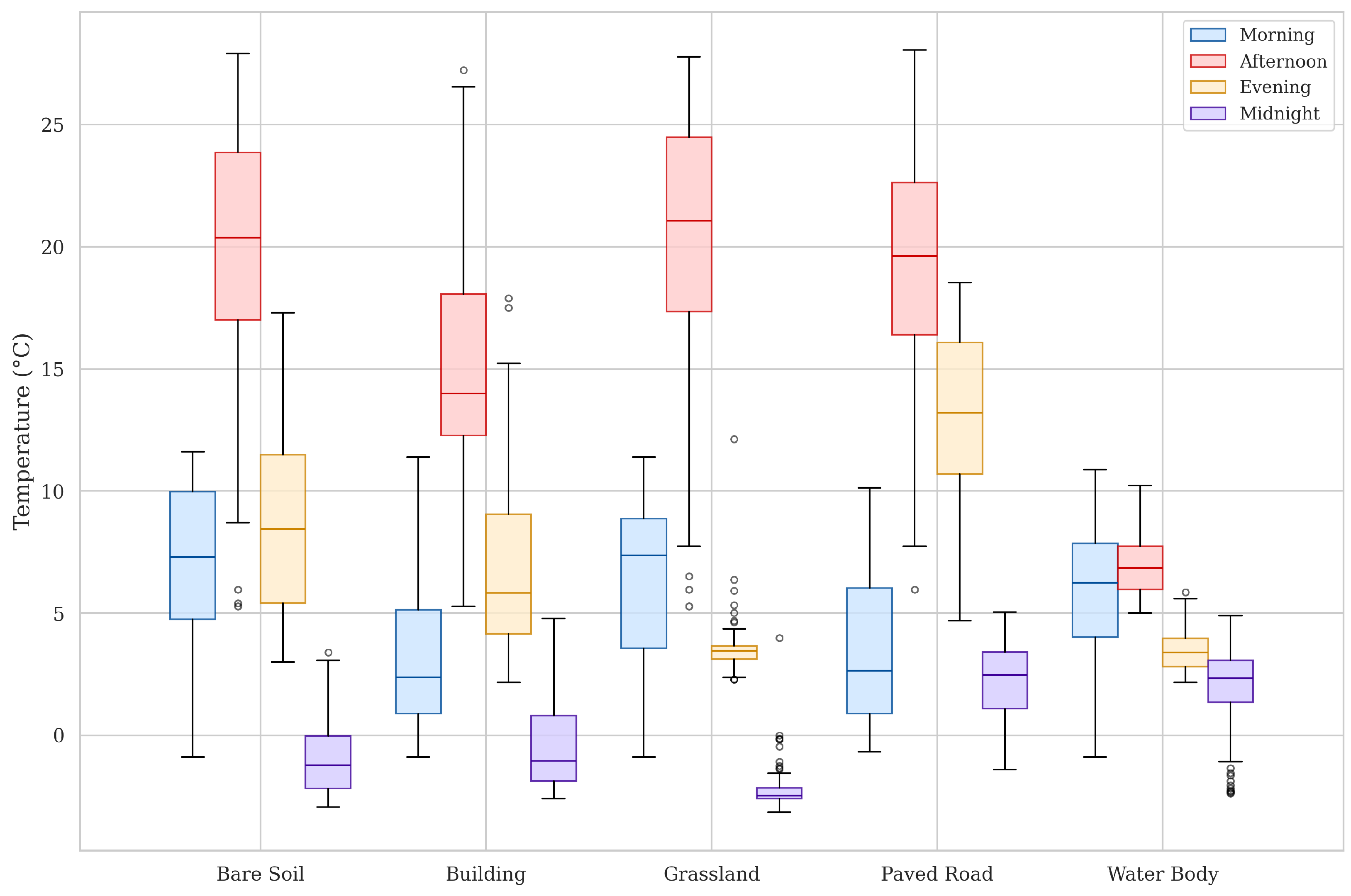
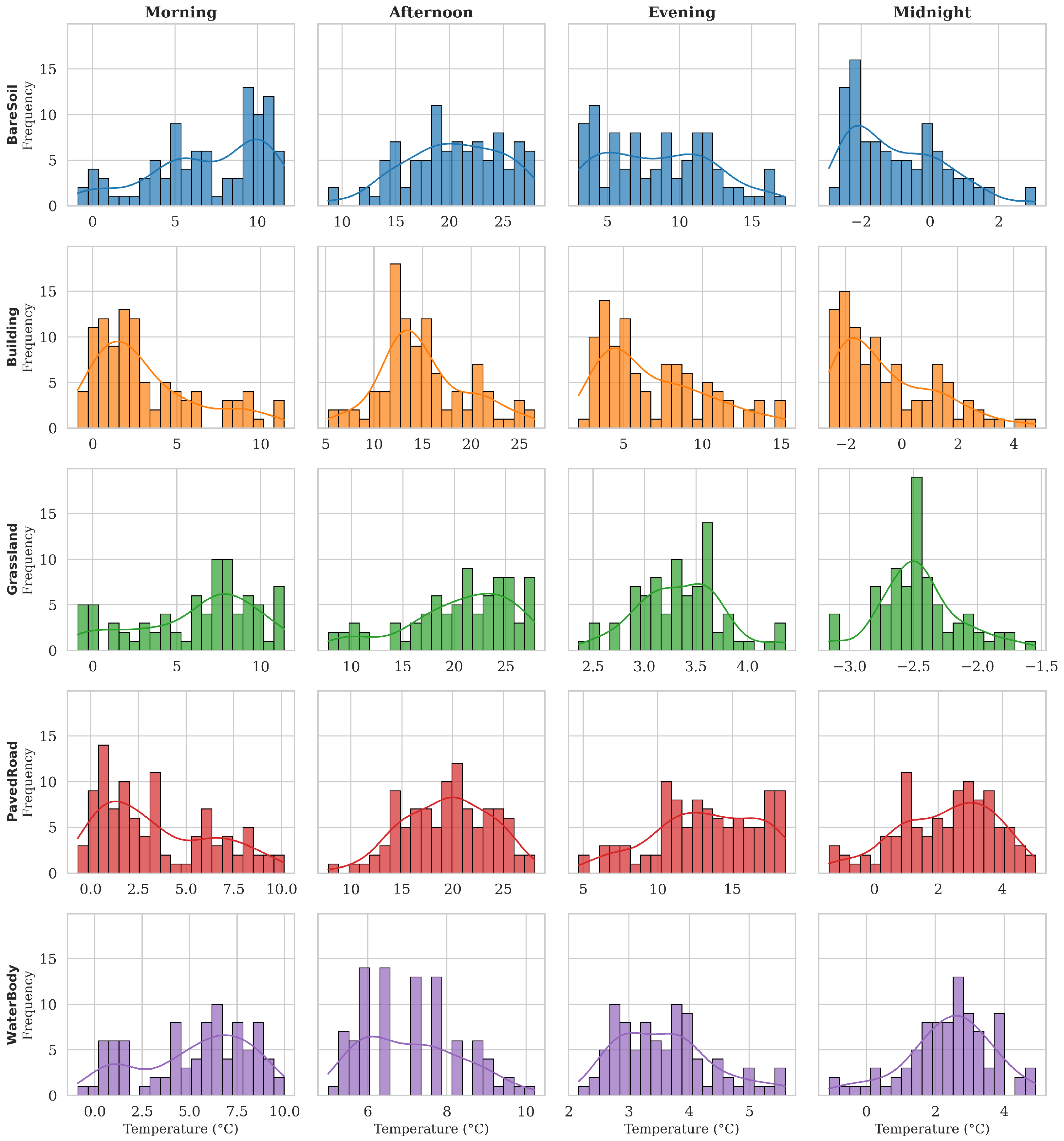
4.2. Frequency Distributions and Descriptive Statistics Analysis

The frequency distributions of LST across different LULC classes and temporal periods revealed distinct thermal behavior patterns, with histograms showing notable variations in distribution shapes and temperature ranges (Figure 5). During morning hours, bare soil and grassland exhibited relatively symmetric distributions centered around 7 °C, while building and paved road surfaces showed positively skewed distributions with peaks at lower temperatures (2–3 °C). Afternoon distributions indicated maximum thermal differentiation, with bare soil, grassland, and paved roads displaying broad, multi-modal distributions spanning 15–25 °C, whereas water bodies maintained a distinctive narrow, concentrated distribution (6–10 °C), reflecting their thermal stability. Evening patterns revealed interesting urban thermal characteristics, particularly in paved roads showing a platykurtic distribution across 5–15 °C, suggesting prolonged heat retention. The midnight distributions were especially noteworthy, with grassland exhibiting a pronounced normal distribution centered at −2.5 °C, while water bodies and paved surfaces maintained positive temperature ranges with right-skewed distributions.

Descriptive statistics of LST by LULC class and temporal period are presented, offering a comprehensive analysis of diurnal LST variations across five distinct LULC classes ($n=463$) as presented in

Table 1. Descriptive statistics of land surface temperature by LULC class and temporal period.

LULC Class	Temporal Period	n	Mean (°C)	SD	Median (°C)	Min	Max
Bare Soil	Morning	96	7.00	3.45	7.45	−0.90	11.62
	Afternoon	96	20.39	4.50	20.78	8.71	27.92
	Evening	96	8.60	3.78	8.57	3.01	17.31
	Midnight	96	−0.97	1.35	−1.18	−2.93	3.07
Building	Morning	98	3.15	3.07	2.38	−0.90	11.39
	Afternoon	98	15.12	4.54	14.06	5.27	26.55
	Evening	98	6.88	3.29	5.79	2.16	15.24
	Midnight	98	−0.52	1.71	−1.05	−2.60	4.78
Grassland	Morning	81	6.19	3.49	7.37	−0.90	11.39
	Afternoon	81	20.57	5.13	21.33	7.75	27.78
	Evening	81	3.34	0.41	3.33	2.36	4.36
	Midnight	81	−2.45	0.31	−2.50	−3.16	−1.55
Paved Road	Morning	99	3.47	2.92	2.75	−0.68	10.13
	Afternoon	99	19.45	4.22	19.69	7.75	28.06
	Evening	99	13.18	3.49	13.23	4.69	18.54
	Midnight	99	2.25	1.51	2.47	−1.41	5.04
Water Body	Morning	89	5.27	2.85	5.95	−0.90	9.98
	Afternoon	89	7.10	1.25	7.20	5.00	10.22
	Evening	89	3.59	0.79	3.52	2.16	5.59
	Midnight	89	2.39	1.25	2.60	−1.08	4.91

Note: SD = Standard Deviation; n = number of observations.

. The results reveal significant temporal and spatial heterogeneity in thermal patterns. Notably, bare soil and grassland exhibited the highest afternoon temperatures (20.39 ± 4.50 °C and 20.57 ± 5.13 °C, respectively), while water bodies demonstrated remarkable thermal stability across all temporal periods (SD range: 0.79–2.85 °C). The maximum thermal amplitude was observed in buildings (ΔT = 21.28 °C during afternoon) and paved roads (ΔT = 20.31 °C during afternoon), indicating strong urban surface heating. Conversely, water bodies maintained the most moderate temperature fluctuations (maximum ΔT = 10.88 °C during morning period), consistent with their high thermal inertia. The midnight period revealed distinct cooling patterns, with grassland showing the lowest temperatures (−2.45 ± 0.31 °C), while paved roads and water bodies retained higher temperatures (2.25 ± 1.51 °C and 2.39 ± 1.25 °C, respectively), suggesting significant human-induced heat retention in urban materials.

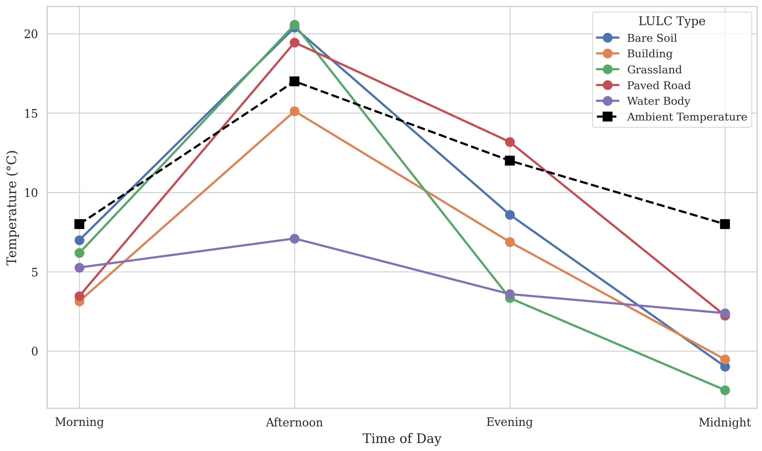
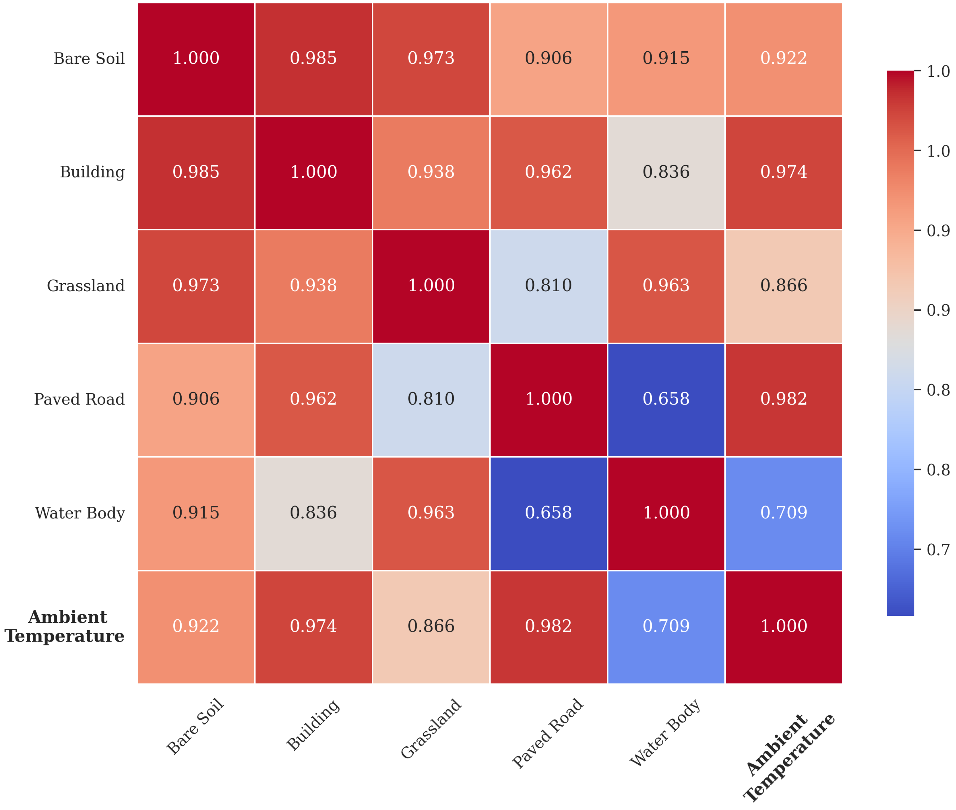
4.3. Trend and Correlation Analysis of LULC and Ambient Temperature

Ambient air temperature measurements were recorded concurrently with the UAV thermal data acquisition flights to establish the relationship between air and land surface temperatures across different temporal periods. The diurnal ambient temperature profile exhibited expected temporal variations, with minimum values recorded during morning and midnight periods (both 8 °C), reaching its peak during afternoon measurements (17 °C), and showing moderate temperatures during the evening period (12 °C). These ambient temperature measurements (single measurement for each time of day) serve as reference data for contextualizing the observed LST patterns and quantifying the surface–air temperature relationships across different LULC classes.

The comparison of LULC class mean temperatures (Figure 6) with ambient weather temperatures revealed significant variations in thermal behavior across different surfaces throughout the diurnal cycle. Bare soil and grassland exhibited the highest fluctuations, with temperatures rising sharply in the afternoon, exceeding ambient conditions, and cooling drastically at midnight. Paved roads demonstrated notable heat retention, maintaining higher temperatures during the evening and midnight hours compared to other LULC classes. Water bodies exhibited the most stable temperature profile, reflecting their high thermal inertia and capacity to moderate temperature fluctuations. Built-up areas, such as buildings, followed a trend similar to ambient temperatures but displayed slightly lower values during the morning and midnight periods. It is possible to say that urban surfaces (paved roads and buildings) retain heat more effectively, contributing to higher evening temperatures, while natural surfaces (bare soil, grassland, and water bodies) respond more dynamically to diurnal temperature variations.

The correlation analysis between LULC classes and ambient temperature revealed significant relationships that provide evidence of the influence of surface types on thermal variations (Figure 7). The results indicated that paved roads and buildings exhibited the strongest correlation with ambient temperature, reinforcing the well-documented urban heat island effect, where artificial surfaces retain and emit heat more intensely than natural landscapes. Urbanization and infrastructural development played a crucial role in modifying the local temperature patterns. In contrast, water bodies showed a weaker correlation with ambient temperature, which aligns with their inherent ability to moderate temperature fluctuations through evaporative cooling and thermal inertia. Furthermore, grasslands and bare soil exhibited moderate correlations, indicating their intermediary role in surface heat absorption and emission dynamics. Building upon these findings, a follow-up analysis examined the correlation between the mean temperature of LULC classes and ambient temperature, revealing a strong positive correlation coefficient of approximately 0.827. The results confirm that as ambient temperature increases, the overall mean temperature across different LULC classes also tends to significantly increase.

4.4. Spatial Autocorrelation Analysis (Moran’s I) Results

Given that sampled points span different LULC classes, it is hypothesized that LST values exhibit spatial clustering due to the thermal properties of various surfaces. To assess the overall spatial dependence of LST across the study area, a global Moran’s I analysis was conducted for four diurnal periods. This approach provides insight into the overall spatial clustering of LST, offering a basis for assessing the suitability of spatially explicit modeling techniques, particularly GWR.

Table 2. Global Moran’s I values for LST across diurnal periods.

Time Period	Moran’s I	p-Value	Interpretation
Morning	0.278	0.001	Moderate clustering
Afternoon	0.560	0.001	Strong clustering
Evening	0.592	0.001	Strong clustering
Midnight	0.604	0.001	Strong clustering

presents the Moran’s I values and their corresponding p-values for each time period. The results indicate statistically significant positive spatial autocorrelation across all timeframes ($p<0.001$), confirming that LST values cluster spatially rather than being randomly distributed.

The analysis shows that spatial autocorrelation in LST strengthens as the day progresses. The Moran’s I value is lowest in the morning (0.278), suggesting that LST distribution is relatively less structured during early hours, likely due to the effects of nocturnal cooling and minimal solar radiation. However, as solar heating intensifies, spatial clustering strengthens, reaching its peak at midnight (0.604), when impervious surfaces and other heat-retaining materials exhibit their maximum residual thermal loads.

The increasing Moran’s I values confirm the presence of structured thermal patterns, highlighting the need for GWR to address spatial dependence in LST variations between LULC categories. The observed clustering indicates that traditional regression models assuming spatial independence would be insufficient, as they would fail to capture the localized effects of different land cover types and their interactions with diurnal temperature variations.

The strong spatial autocorrelation in LST has key implications for the subsequent analytical approach. The significant spatial autocorrelation observed directly justifies the adoption of GWR as the primary spatial analytical technique in this study. GWR effectively models spatial non-stationarity and dependence, making it well suited for analyzing the spatially varying relationships between LULC and LST.

4.5. GWR Results

Following the Moran’s I analysis, which demonstrated significant spatial autocorrelation in LST across various LULC classes and diurnal periods, GWR was applied to explore the spatially varying relationships between LULC proximity and LST. The results of the GWR analysis are presented in both graphical and tabular formats to provide a comprehensive view of the spatial and temporal dynamics. Figure 8 displays a heat map of $R^2$ values, offering a visual representation of the model’s explanatory power across different LULC classes and timeframes. In parallel,

Table 3. Detailed GWR analysis across LULC classes and timeframes.

LULC Class	Timeframe	Bandwidth	Adjusted R2
Bare Soil	Morning	67.0	0.142
	Afternoon	94.0	−0.053
	Evening	81.0	0.515
	Midnight	73.0	0.460
Building	Morning	79.0	0.149
	Afternoon	80.0	0.162
	Evening	94.0	0.231
	Midnight	86.0	0.255
Grassland	Morning	80.0	0.057
	Afternoon	77.0	0.227
	Evening	80.0	0.030
	Midnight	80.0	−0.010
Paved Road	Morning	57.0	0.246
	Afternoon	92.0	0.403
	Evening	81.0	0.567
	Midnight	76.0	0.514
Water Body	Morning	53.0	0.617
	Afternoon	57.0	0.339
	Evening	57.0	0.638
	Midnight	53.0	0.550

details the optimal bandwidth settings and corresponding adjusted $R^2$ values for each LULC class across time periods. These metrics define the spatial scale at which local regression relationships are estimated and highlight the model’s explanatory power, along with its variations across different times of the day.

For areas dominated by bare soil, the strength of the spatial relationship with temperature varies considerably throughout the day. In the morning, the GWR model for bare soil explains approximately 14% of the variance (adjusted $R^2\approx 0.14$, $R^2\approx 0.24$), suggesting a moderate level of local explanatory power. However, during the afternoon, the explanatory power drops dramatically (adjusted $R^2\approx -0.05$, $R^2\approx 0.03$), which implies that factors other than proximity to bare soil may be more influential during this period, or that the relationship is more complex and less linear. In contrast, the evening and midnight periods show a substantial improvement in model fit (adjusted $R^2\approx 0.515$ and $0.460$, respectively), indicating that bare soil proximity is more strongly associated with temperature variations later in the day. The GWR bandwidth for bare soil also varies (ranging from 67 in the morning to 94 in the afternoon), suggesting that the spatial scale over which bare soil influences temperature is not constant and may depend on diurnal environmental processes.

For built-up areas, the GWR models consistently capture a moderate proportion of the variance in temperature across all timeframes. The morning model (adjusted $R^2\approx 0.149$, $R^2\approx 0.23$) and the afternoon model (adjusted $R^2\approx 0.162$, $R^2\approx 0.24$) indicate a similar level of association. There is a modest increase in the model performance during the evening (adjusted $R^2\approx 0.231$, $R^2\approx 0.29$) and midnight (adjusted $R^2\approx 0.255$, $R^2\approx 0.32$) timeframes. The relatively stable but slightly increasing adjusted $R^2$ values suggest that the influence of proximity to buildings on temperature might become slightly more pronounced later in the day, possibly due to heat retention and nocturnal cooling dynamics. The bandwidth values (ranging from 79 to 94) imply that the spatial extent of the building-related effects is moderately broad.

Grasslands display the weakest and most inconsistent relationships with temperature. In the morning, the model explains only about 6% of the variance (adjusted $R^2\approx 0.057$, $R^2\approx 0.14$). The afternoon period shows better performance (adjusted $R^2\approx 0.227$, $R^2\approx 0.30$), but the evening and midnight models drop again to adjusted $R^2$ values of approximately $0.030$ and $-0.010$, respectively. The negative adjusted $R^2$ value for the grassland midnight model ($-0.010$) indicates that this model performs worse than a simple average in explaining LST variations, suggesting that, at midnight for grasslands, proximity to the considered LULC types is not a useful predictor of temperature. These low adjusted $R^2$ values overall indicate that proximity to grasslands has a minimal and unstable association with temperature variations, suggesting that other environmental or human-induced factors may override any potential cooling or warming effects of grassland areas. The bandwidth for grassland remains relatively consistent (around 77–80), indicating a uniform spatial scale that, however, does not translate into a strong explanatory relationship.

Paved roads demonstrate a relatively robust association with temperature variations, particularly during the afternoon, evening, and midnight periods. The morning model yields an adjusted $R^2$ of about $0.246$ ($R^2\approx 0.35$), but this increases to approximately $0.403$ in the afternoon, peaks at about $0.567$ in the evening, and remains high at $0.514$ at midnight. These elevated adjusted $R^2$ values suggest that the thermal effects associated with paved surfaces—possibly due to heat absorption and retention—are more pronounced later in the day. The varying bandwidth (from 57 in the morning to 92 in the afternoon) indicates that the spatial influence of paved roads is not uniform throughout the day, potentially reflecting differences in urban morphology or surface material properties that affect heat storage and release.

Among the LULC types examined, proximity to water bodies shows the strongest and most consistent relationship with temperature variation. In the morning, the model explains roughly 62% of the variance (adjusted $R^2\approx 0.617$, $R^2\approx 0.68$), and similarly high values are observed in the evening (adjusted $R^2\approx 0.638$, $R^2\approx 0.69$) and midnight (adjusted $R^2\approx 0.550$, $R^2\approx 0.62$) periods. The afternoon model, while lower (adjusted $R^2\approx 0.339$, $R^2\approx 0.44$), still suggests a substantial association. The consistently high adjusted $R^2$ values imply that water bodies exert a strong localized influence on temperature, likely due to their capacity to moderate local climates through evaporative cooling and thermal inertia. This inference is supported by the relatively small bandwidth values (53–57), indicating that the cooling effect of water bodies is highly localized.

To quantify the temporal variations in LULC thermal influence, we calculated the percentage changes in adjusted $R^2$ values between consecutive time periods (

Table 4. Percentage changes in adjusted $R^2$ values between consecutive time periods for different LULC classes.

LULC Class	Morning to Afternoon	Afternoon to Evening	Evening to Midnight	Mean Adjusted ${\mathit{R}}^2$
Bare Soil	−137.3%	+1071.7%	−10.7%	0.266
Building	+8.7%	+42.6%	+10.4%	0.199
Grassland	+298.2%	−86.8%	−133.3%	0.076
Paved Road	+63.8%	+40.7%	−9.3%	0.433
Water Body	−45.1%	+88.2%	−13.8%	0.536

Note: Values represent percentage changes in adjusted $R^2$ between consecutive time periods. Positive values indicate strengthening relationships, while negative values indicate weakening relationships.

). The most pronounced temporal shift occurred in bare soil, which experienced a dramatic decrease from morning to afternoon ($-137.3\%$), followed by a substantial recovery in the evening period ($+1071.7\%$). Water bodies demonstrated notable diurnal fluctuation patterns with a $45.1\%$ decrease in explanatory power from morning to afternoon, followed by an $88.2\%$ increase from afternoon to evening, highlighting their dynamic role in thermal regulation throughout the day. Paved roads showed consistent strengthening of thermal relationships across the daily cycle, with increases of $63.8\%$ from morning to afternoon and a further $40.7\%$ from afternoon to evening, before a slight decline ($-9.3\%$) at midnight. Comparing across LULC types, water bodies exhibited the strongest overall thermal influence, with mean adjusted $R^2$ of 0.536 across all time periods, followed by paved roads (0.433), while grassland showed the weakest overall relationship (0.076). The most pronounced thermal relationship for any LULC–time combination was observed for water bodies during evening hours (adjusted $R^2=0.638$), which was 21.3 times stronger than the weakest significant relationship (grassland during evening, adjusted $R^2=0.030$). These quantitative differences in model performance across time periods substantiate the temporal dependence of thermal relationships and highlight critical transitions, particularly the evening period (17:00–18:00) when thermal influence patterns undergo significant reconfiguration across most LULC classes.

The results underscore that the thermal influence of various LULC types is both temporally and spatially heterogeneous. The high explanatory power of the models for water bodies and paved roads—especially during periods of lower solar radiation (evening and midnight)—suggests that these features play significant roles in modulating local temperatures. In contrast, the variable performance for bare soils and the generally weak associations for grasslands highlight that the effects of these land covers are more context dependent, potentially influenced by additional factors such as moisture content, albedo variations, or adjacent land uses.

5. Discussion

According to the high-resolution results of this study, the pronounced heat retention capabilities of impervious surfaces substantiate the fundamental mechanisms underlying urban heat island formation. Paved roads and buildings demonstrate substantial thermal inertia, maintaining elevated temperatures into evening and midnight periods despite ambient cooling. This persistence aligns with theoretical understanding of materials with high volumetric heat capacity and low albedo, which function as urban heat reservoirs. In this case, it can be said that the energy balance reflects a process where the radiation absorbed during daylight hours is gradually released at night. The Moran’s I results are derived from a global spatial autocorrelation analysis rather than individual LULC class-based assessments. This approach allows for a broader evaluation of how the spatial clustering of LST evolves across different diurnal periods, independent of land cover classifications. The significant increase in Moran’s I values from morning to midnight highlights the progressive spatial structuring of thermal anomalies over time, further justifying the necessity of spatially explicit modeling techniques such as GWR. GWR modeling reveals that thermal influence extends beyond immediate adjacencies, suggesting human-made surfaces create thermal footprints beyond their physical boundaries.

In contrast, natural landscapes demonstrate distinctive thermal regulation mechanisms. Water bodies exhibit exceptional thermal stability throughout the diurnal cycle—attributable to water’s unique thermophysical properties. The high specific heat capacity and thermal conductivity create a buffering effect that modulates temperature extremes through multiple pathways: absorption of substantial heat energy with minimal temperature change, vertical mixing that distributes heat throughout the water column, and evaporative cooling that dissipates energy through phase changes. GWR models reveal that water bodies exert highly localized cooling influences, suggesting a “thermal oasis” effect that diminishes rapidly with distance—a pattern differing markedly from the broader thermal influence zones of paved surfaces. The strong positive spatial autocorrelation observed in water bodies indicates internally consistent thermal behavior that could be strategically leveraged in urban design.

Vegetated surfaces present another thermal archetype, with grasslands demonstrating remarkable nocturnal cooling efficiency through evapotranspiration, radiative cooling, and limited heat storage capacity. The weaker spatial autocorrelation in grassland areas suggests greater thermal heterogeneity, likely stemming from variations in vegetation density, soil moisture content, and microscale topography. The anomalous negative spatial autocorrelation detected in bare soil during afternoon periods reveals counterintuitive thermal patterning where dissimilar temperature values cluster adjacently, suggesting complex microscale dynamics driven by variations in soil composition, moisture gradients, and surface roughness.

The application of SfM photogrammetry for thermal orthomosaic generation introduces specific methodological complexities that warrant careful consideration. Unlike visible spectrum imagery for which SfM algorithms are primarily designed, thermal infrared data present distinct challenges including lower spatial resolution, reduced textural detail, and temperature-dependent radiometric variations that can affect feature detection and matching processes. To address these limitations, we implement several targeted mitigation strategies during our workflow: (1) the optimization of flight parameters with increased image overlap (90% compared to the standard 60–70% for RGB imagery) to enhance point cloud density; (2) the application of specialized feature detection algorithms calibrated for thermal contrast rather than visual texture; and (3) temporal consistency controls ensuring minimal temperature variation during each flight mission (limited to <45 min).

Several methodological aspects of the study warrant consideration. The SfM photogrammetry approach for thermal orthomosaic generation introduces additional complexity, as thermal infrared wavelength characteristics differ fundamentally from visible spectrum imagery for which most SfM algorithms are optimized. The temporal scope of this study—limited to a single day in January within a semiarid climate—constrains generalizability to different seasons or climatic regimes. This limitation is particularly significant when considering that surface thermal properties can vary substantially with seasonal environmental conditions. For instance, vegetated surfaces demonstrate markedly different thermal signatures during growing seasons due to changes in leaf area index and evapotranspiration rates. Similarly, the thermal behavior of impervious surfaces may differ under summer conditions with increased solar radiation and higher ambient temperatures. Furthermore, seasonal variations in soil moisture content likely influence the thermal response of bare soil areas. While our January measurements effectively capture winter thermal dynamics and provide valuable insights into surface material properties with minimal vegetation influence, they represent only one temporal snapshot in the annual climatic cycle. Additionally, a detailed local assessment focusing on class-based spatial autocorrelation patterns may yield deeper insights into the spatial heterogeneity of thermal behaviors across specific LULC types.

The empirical quantification of LULC-specific thermal signatures offers valuable guidance for urban climate adaptation strategies. The observed prolonged heat retention in impervious surfaces substantiates the efficacy of several interventions: deployment of high-albedo materials, implementation of permeable pavements, and strategic integration of green infrastructure. The temporal persistence of elevated temperatures in paved surfaces into evening and midnight periods highlights the importance of considering nocturnal thermal comfort in urban design—particularly critical given climate change projections that indicates disproportionate increases in nighttime temperature minima. The proven cooling effect of water bodies underscores the importance of incorporating water-based elements into urban planning, with GWR models facilitating data-driven optimization of hydrological features. The considerable spatial variability in thermal patterns indicates that urban cooling strategies should be tailored to specific locations rather than applied uniformly.

6. Conclusions

This investigation has demonstrated the efficacy of high-resolution UAV thermal remote sensing for characterizing diurnal LST variations across heterogeneous urban landscapes. Through the systematic examination of five distinct LULC classes at four critical diurnal periods, the research has yielded statistically robust insights into surface-specific thermal behavior patterns with implications for urban microclimate management.

The findings reveal fundamental thermal behavior distinctions between artificial and natural surfaces that directly impact urban heat dynamics. Impervious surfaces exhibited pronounced heat retention capabilities, with paved roads maintaining elevated temperatures during evening and midnight periods despite ambient cooling—a key mechanism underlying persistent nocturnal urban heat islands. Water bodies demonstrated exceptional thermal stability, while vegetated surfaces showed efficient nocturnal cooling. These class-specific thermal signatures were further validated through spatial autocorrelation analysis (Moran’s I) and GWR modeling, which identified spatially heterogeneous relationships between LST and LULC distribution patterns.

The methodological approach developed in this study—integrating UAV-based thermal orthomosaic generation with stratified random sampling, robust outlier management, and spatially explicit modeling—advances urban microclimate monitoring capabilities beyond traditional satellite-based approaches. The GWR models revealed that water bodies exerted the strongest localized cooling influence, while impervious surfaces demonstrated significant heat-retention effects persisting into nocturnal periods—quantifications that provide critical benchmarks for urban climate models.

These empirically validated thermal signatures offer actionable guidance for climate-adaptive urban planning interventions. The documented prolonged heat retention in paved surfaces substantiates the need for implementing high-albedo materials and permeable pavements in heat-vulnerable urban areas. The exceptional thermal stability of water bodies supports strategic integration of water features as microclimate regulators, with their highly localized cooling influence (as revealed by GWR bandwidths of 53–57) informing optimal spatial placement. The variable cooling rates across LULC types indicate that urban design should incorporate temporal considerations—scheduling heat-sensitive urban activities in areas dominated by surfaces with efficient nocturnal cooling properties. Furthermore, the significant spatial variability in thermal patterns revealed by our Moran’s I analysis demonstrates that urban cooling strategies must be spatially targeted rather than uniformly applied, with particular attention to impervious surface clustering that intensifies heat island effects.

Future research directions should include the following: (1) multi-seasonal observations to capture thermal behavior under varying meteorological conditions; (2) the integration of in situ validation instrumentation to enhance measurement accuracy; (3) the inclusion of three-dimensional morphological parameters to account for urban geometric effects; and (4) coupling thermal measurements with human bioclimatic indices to translate physical observations into health-relevant metrics. Such advancements would further contribute to comprehensive understanding of urban thermal environments and support evidence-based strategies for sustainable, climate-resilient urban development.

References

1. Meerow, S.; Newell, J.P.; Stults, M. Defining urban resilience: A review. Landsc. Urban Plan. 2019, 147, 38–49. [Google Scholar] [CrossRef]
2. McPhearson, T.; Iwaniec, D.M.; Bai, X. Positive visions for guiding urban transformations toward sustainable futures. Curr. Opin. Environ. Sustain. 2018, 22, 33–40. [Google Scholar] [CrossRef]
3. He, B.J.; Zhao, D.X.; Zhu, J.; Darko, A.; Gou, Z. Promoting and implementing urban sustainability in China: An integration of sustainable initiatives at different urban scales. Habitat Int. 2021, 82, 83–93. [Google Scholar] [CrossRef]
4. Wang, F.; Qin, Z.; Song, C.; Tu, L.; Karnieli, A.; Zhao, S. An improved mono-window algorithm for land surface temperature retrieval from Landsat 8 thermal infrared sensor data. Remote Sens. 2015, 7, 4268–4289. [Google Scholar] [CrossRef]
5. Yao, H.; Qin, R.; Chen, X. Unmanned aerial vehicle for remote sensing applications—A review. Remote Sens. 2019, 11, 1443. [Google Scholar] [CrossRef]
6. Feng, Y.; Du, S.; Myint, S.W.; Shu, M. Do urban functional zones affect land surface temperature differently? A case study of Beijing, China. Remote Sens. 2019, 11, 1802. [Google Scholar] [CrossRef]
7. Burger, M.; Gubler, M.; Heinimann, A.; Brönnimann, S. Modelling the spatial pattern of heatwaves in the city of Bern using a land use regression approach. Urban Clim. 2021, 38, 100885. [Google Scholar] [CrossRef]
8. Chudnovsky, A.; Ben-Dor, E.; Saaroni, H. Diurnal thermal behavior of selected urban objects using remote sensing measurements. Energy Build. 2004, 36, 1063–1074. [Google Scholar] [CrossRef]
9. Yin, C.; Yuan, M.; Lu, Y.; Huang, Y.; Liu, Y. Effects of urban form on the urban heat island effect based on spatial regression model. Sci. Total Environ. 2018, 634, 696–704. [Google Scholar] [CrossRef]
10. Conti, S.; Meli, P.; Minelli, G.; Solimini, R.; Toccaceli, V.; Vichi, M.; Beltrano, C.; Perini, L. Epidemiologic study of mortality during the summer 2003 heat wave in Italy. Environ. Res. 2005, 98, 390–399. [Google Scholar]
11. Davarzani, H.; Smits, K.; Tolene, R.M.; Illangasekare, T. Study of the effect of wind speed on evaporation from soil through integrated modeling of the atmospheric boundary layer and shallow subsurface. Water Resour. Res. 2014, 50, 661–680. [Google Scholar] [CrossRef]
12. Wang, W.Z.; Liu, L.C.; Liao, H.; Wei, Y.M. Impacts of urbanization on carbon emissions: An empirical analysis from OECD countries. Energy Policy 2021, 151, 112171. [Google Scholar] [CrossRef]
13. Ren, Y.; Deng, L.Y.; Zuo, S.D.; Song, X.D.; Liao, Y.L.; Xu, C.D.; Chen, Q.; Hua, L.Z.; Li, Z.W. Quantifying the influences of various ecological factors on land surface temperature of urban forests. Environ. Pollut. 2016, 216, 519–529. [Google Scholar] [CrossRef]
14. Xu, S.; Yang, K.; Xu, Y.; Zhu, Y.; Luo, Y.; Shang, C.; Zhang, J.; Zhang, Y.; Gao, M.; Wu, C. Urban land surface temperature monitoring and surface thermal runoff pollution evaluation using UAV thermal remote sensing technology. Sustainability 2021, 13, 11203. [Google Scholar] [CrossRef]
15. Santesteban, L.G.; Di Gennaro, S.F.; Herrero-Langreo, A.; Miranda, C.; Royo, J.B.; Matese, A. High-resolution UAV-based thermal imaging to estimate the instantaneous and seasonal variability of plant water status within a vineyard. Agric. Water Manag. 2017, 183, 49–59. [Google Scholar] [CrossRef]
16. Ortiz-Sanz, J.; Gil-Docampo, M.; Arza-García, M.; Cañas-Guerrero, I. IR thermography from UAVs to monitor thermal anomalies in the envelopes of traditional wine cellars: Field test. Remote Sens. 2019, 11, 1424. [Google Scholar] [CrossRef]
17. Perich, G.; Hund, A.; Anderegg, J.; Roth, L.; Boer, M.P.; Walter, A.; Liebisch, F.; Aasen, H. Assessment of multi-image unmanned aerial vehicle based high-throughput field phenotyping of canopy temperature. Front. Plant Sci. 2020, 11, 150. [Google Scholar] [CrossRef]
18. Nieto, H.; Kustas, W.P.; Torres-Rúa, A.; Alfieri, J.G.; Gao, F.; Anderson, M.C.; White, W.A.; Song, L.; Alsina, M.d.M.; Prueger, J.H.; et al. Evaluation of TSEB turbulent fluxes using different methods for the retrieval of soil and canopy component temperatures from UAV thermal and multispectral imagery. Irrig. Sci. 2019, 37, 389–406. [Google Scholar] [CrossRef]
19. Casana, J.; Wiewel, A.; Cool, A.; Hill, C.; Fisher, K.D.; Laugier, E.J. Archaeological aerial thermography in theory and practice. Adv. Archaeol. Pract. 2017, 5, 310–327. [Google Scholar] [CrossRef]
20. Zheng, H.; Zhong, X.; Yan, J.; Zhao, L.; Wang, X. A thermal performance detection method for building envelope based on 3D model generated by UAV thermal imagery. Energies 2020, 13, 6677. [Google Scholar] [CrossRef]
21. Kelly, J.; Kljun, N.; Olsson, P.-O.; Mihai, L.; Liljeblad, B.; Weslien, P.; Klemedtsson, L.; Eklundh, L. Challenges and best practices for deriving temperature data from an uncalibrated UAV thermal infrared camera. Remote Sens. 2019, 11, 567. [Google Scholar] [CrossRef]
22. Acorsi, M.G.; Gimenez, L.M.; Martello, M. Assessing the performance of a low-cost thermal camera in proximal and aerial conditions. Remote Sens. 2020, 12, 3591. [Google Scholar] [CrossRef]
23. Aragon, B.; Johansen, K.; Parkes, S.; Malbeteau, Y.; Al-Mashharawi, S.; Al-Amoudi, T.; Andrade, C.F.; Turner, D.; Lucieer, A.; McCabe, M.F. A calibration procedure for field and UAV-based uncooled thermal infrared instruments. Sensors 2020, 20, 3316. [Google Scholar] [CrossRef] [PubMed]
24. Henn, K.A.; Peduzzi, A. Surface heat monitoring with high-resolution UAV thermal imaging: Assessing accuracy and applications in urban environments. Remote Sens. 2024, 16, 930. [Google Scholar] [CrossRef]
25. Song, B.; Park, K. Verification of accuracy of unmanned aerial vehicle (UAV) land surface temperature images using in-situ data. Remote Sens. 2020, 12, 288. [Google Scholar] [CrossRef]
26. Lee, K.; Lee, W.H. Temperature accuracy analysis by land cover according to the angle of the thermal infrared imaging camera for unmanned aerial vehicles. ISPRS Int. J. Geo-Inf. 2022, 11, 204. [Google Scholar] [CrossRef]
27. Naughton, J.; McDonald, W. Evaluating the variability of urban land surface temperatures using drone observations. Remote Sens. 2019, 11, 1722. [Google Scholar] [CrossRef]
28. Soto-Estrada, E.; Correa-Echeverri, S.; Posada-Posada, M.I. Thermal analysis of urban environments in Medellin, Colombia, using an unmanned aerial vehicle (UAV). J. Urban Environ. Eng. 2017, 11, 142–149. [Google Scholar] [CrossRef]
29. Ahmad, J.; Sajjad, M.; Eisma, J. Small unmanned aerial vehicle (UAV)-based detection of seasonal micro-urban heat islands for diverse land uses. Int. J. Remote Sens. 2025, 46, 119–147. [Google Scholar] [CrossRef]
30. Lee, K.; Park, J.; Jung, S.; Lee, W. Roof color-based warm roof evaluation in cold regions using a UAV-mounted thermal infrared imaging camera. Energies 2021, 14, 6488. [Google Scholar] [CrossRef]
31. Son, S.; Kim, D. Utilizing high-resolution UAV thermal imaging for land use and land cover-based land surface temperature analysis in urban parks. Landsc. Ecol. Eng. 2024. [CrossRef]
32. Yang, J.; Wang, Y.; Xue, B.; Li, Y.; Xiao, X.; Xia, J.C.; He, B. Contribution of urban ventilation to the thermal environment and urban energy demand: Different climate background perspectives. Sci. Total Environ. 2021, 795, 148791. [Google Scholar] [CrossRef] [PubMed]
33. Smith, P.; Sarricolea, P.; Peralta, O.; Aguila, J.P.; Thomas, F. Study of the urban microclimate using thermal UAV: The case of the mid-sized cities of Arica (arid) and Curicó (Mediterranean), Chile. Build. Environ. 2021, 206, 108372. [Google Scholar] [CrossRef]
34. Kim, D.; Yu, J.; Yoon, J.; Jeon, S.; Son, S. Comparison of accuracy of surface temperature images from unmanned aerial vehicles and satellites for precise thermal environment monitoring of urban parks using in situ data. Remote Sens. 2021, 13, 1977. [Google Scholar] [CrossRef]
35. Ahmad, J.; Eisma, J.A. Capturing small-scale surface temperature variation across diverse urban land uses with a small unmanned aerial vehicle. Remote Sens. 2023, 15, 2042. [Google Scholar] [CrossRef]
36. Wang, X.; Prigent, C. Comparisons of diurnal variations of land surface temperatures from numerical weather prediction analyses, infrared satellite estimates, and in situ measurements. Remote Sens. 2020, 12, 583. [Google Scholar] [CrossRef]
37. Qian, F.; Hu, Y.; Wu, R.; Yan, H.; Wang, D.; Xiang, Z.; Zhao, K.; Han, Q.; Shao, F.; Bao, Z. Assessing the spatial-temporal impacts of underlying surfaces on 3D thermal environment: A field study based on UAV vertical measurements. Build. Environ. 2024, 265, 111985. [Google Scholar] [CrossRef]
38. Malbéteau, Y.; Parkes, S.; Aragon, B.; Rosas, J.; McCabe, M.F. Capturing the diurnal cycle of land surface temperature using an unmanned aerial vehicle. Remote Sens. 2018, 10, 1407. [Google Scholar] [CrossRef]
39. Wu, Y.; Shan, Y.; Lai, Y.; Zhou, S. Method of calculating land surface temperatures based on low-altitude UAV thermal infrared remote sensing data and near-ground meteorological data. Sustain. Cities Soc. 2022, 78, 103615. [Google Scholar] [CrossRef]
40. Meteoroloji Genel Müdürlüğü. Yeni Köppen İklim Sınıflandırması Haritası. 2023. Available online: https://www.mgm.gov.tr/files/iklim/iklim_siniflandirmalari/koppen.pdf (accessed on 8 March 2025).
41. Koppen Earth Project. Koeppen-Geiger Climate Classification Map. 2025. Available online: https://koppen.earth/ (accessed on 8 March 2025).
42. Beck, H.E.; McVicar, T.R.; Vergopolan, N.; de Jong, R.A.F.; van Dijk, A.; Bastos, A.I.; Miralles, D.G.; Wang, G.; Zhang, J.; Reichstein, M.; et al. High-resolution (1 km) Köppen-Geiger maps for 1901–2099 based on constrained CMIP6 projections. Sci. Data 2023, 10, 724. [Google Scholar] [CrossRef]
43. DJI. Specs–DJI Mavic 3 Enterprise. DJI Enterprise. 2025. Available online: https://enterprise.dji.com/mavic-3-enterprise/specs (accessed on 17 February 2025).
44. Westoby, M.J.; Brasington, J.; Glasser, N.F.; Hambrey, M.J.; Reynolds, J.M. ‘Structure-from-Motion’photogrammetry: A low-cost, effective tool for geoscience applications. Geomorphology 2012, 179, 300–314. [Google Scholar] [CrossRef]
45. James, M.R.; Robson, S.; d’Oleire Oltmanns, S.; Niethammer, U. Optimising UAV topographic surveys processed with structure-from-motion: Ground control quality, quantity and bundle adjustment. Geomorphology 2017, 280, 51–66. [Google Scholar] [CrossRef]
46. Tukey, J.W. Exploratory Data Analysis; Addison-Wesley: Boston, MA, USA, 1977. [Google Scholar]
47. Iglewicz, B.; Hoaglin, D.C. How to Detect and Handle Outliers; ASQC Quality Press: Milwaukee, WI, USA, 1993. [Google Scholar]
48. Moran, P.A.P. Notes on Continuous Stochastic Phenomena. Biometrika 1950, 37, 17–23. [Google Scholar] [CrossRef] [PubMed]
49. Cliff, A.D.; Ord, J.K. Spatial Processes: Models & Applications; Pion: London, UK, 1981. [Google Scholar]
50. Anselin, L. Local Indicators of Spatial Association—LISA. Geogr. Anal. 1995, 27, 93–115. [Google Scholar] [CrossRef]
51. Fotheringham, A.S.; Brunsdon, C.; Charlton, M. Geographically Weighted Regression: The Analysis of Spatially Varying Relationships; Wiley: Hoboken, NJ, USA, 2002. [Google Scholar]
52. Wheeler, D.; Tiefelsdorf, M. Multicollinearity and correlation among local regression coefficients in geographically weighted regression. J. Geogr. Syst. 2005, 7, 161–187. [Google Scholar] [CrossRef]
53. Bentley, J.L. Multidimensional binary search trees used for associative searching. Commun. ACM 1975, 18, 509–517. [Google Scholar] [CrossRef]
54. Kiefer, J. Sequential minimax search for a maximum. Proc. Am. Math. Soc. 1953, 4, 502–506. [Google Scholar] [CrossRef]
Figure 1. Study area of Harran University Osmanbey Campus.
Applsci 15 03448 g001
Figure 2. Spatial distribution of sample points within the Harran University Osmanbey Campus study area. Sample points are color-coded by LULC class (depicted in the legend) and presented for zoomed-in locations representing the following: bare soil, buildings, grassland, paved roads, and water bodies.
Applsci 15 03448 g002
Figure 3. Thermal orthophotos of the Harran University Osmanbey Campus illustrating LST distribution at four diurnal periods: (a) morning, (b) afternoon, (c) evening, (d) midnight.
Applsci 15 03448 g003
Figure 4. Box-and-whisker plots depicting the diurnal LST distribution across five LULC classes (bare soil, building, grassland, paved road, and water body) measured during four temporal periods (morning, afternoon, evening, and midnight).
Applsci 15 03448 g004
Figure 5. Frequency distributions of LST across five LULC classes (bare soil, building, grassland, paved road, and water body) during four diurnal periods (morning, afternoon, evening, and midnight). The histograms with overlaid kernel density estimates illustrate distinct thermal signatures and temporal evolution patterns.
Applsci 15 03448 g005
Figure 6. Diurnal temperature variations across different LULC classes compared to ambient temperature measurements. The graph illustrates the temporal evolution of surface temperatures for bare soil, building, grassland, paved road, and water body surfaces alongside ambient air temperature (dashed line) across four temporal periods (morning, afternoon, evening, and midnight).
Applsci 15 03448 g006
Figure 7. Correlation matrix depicting the statistical relationships between different LULC classes and ambient temperature. Values range from −1 to 1, with darker red indicating stronger positive correlations and blue representing weaker correlations. The diagonal represents perfect self-correlation (1.00).
Applsci 15 03448 g007
Figure 8. Heatmap of local R 2 values from GWR models evaluating the spatially varying influence of LULC proximity on LST. Color intensity corresponds to the magnitude of the local R 2 values, with darker shades indicating stronger local explanatory power.
Applsci 15 03448 g008