


Applying Spectral Clustering to Decode Mobility Patterns in Athens, Greece


Abstract
:1. Introduction
2. Data and Methods
2.1. Spectral Clustering Analysis
2.2. Data Collection and Processing
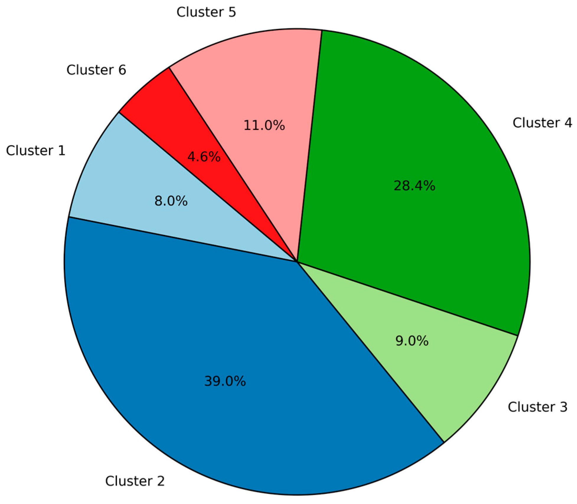
3. Results
4. Discussion
4.1. Clusters’ Interpretation and Main Findings
4.2. Study Limitations
4.3. Scientific and Practical Recommendations
5. Conclusions
Author Contributions
Funding
Institutional Review Board Statement
Informed Consent Statement
Data Availability Statement
Acknowledgments
Conflicts of Interest
Appendix A

References
- Knowles, R.D.; Ferbrache, F.; Nikitas, A. Transport’s Historical, Contemporary and Future Role in Shaping Urban Development: Re-Evaluating Transit Oriented Development. Cities 2020, 99, 102607. [Google Scholar] [CrossRef]
- Tsigdinos, S.; Tzouras, P.G.; Bakogiannis, E.; Kepaptsoglou, K.; Nikitas, A. The Future Urban Road: A Systematic Literature Review-Enhanced Q-Method Study with Experts. Transp. Res. Part D Transp. Environ. 2022, 102, 103158. [Google Scholar] [CrossRef]
- Peeters, P.; Dubois, G. Tourism Travel under Climate Change Mitigation Constraints. J. Transp. Geogr. 2010, 18, 447–457. [Google Scholar] [CrossRef]
- Gurram, S.; Stuart, A.L.; Pinjari, A.R. Agent-Based Modeling to Estimate Exposures to Urban Air Pollution from Transportation: Exposure Disparities and Impacts of High-Resolution Data. Comput. Environ. Urban Syst. 2019, 75, 22–34. [Google Scholar] [CrossRef]
- SÒlensminde, K. Stated Choice Valuation of Urban traffic Air Pollution and Noise. Transp. Res. Part D Transp. Environ. 1999, 4, 13–27. [Google Scholar]
- Müller, J.; Straub, M.; Richter, G.; Rudloff, C. Integration of Different Mobility Behaviors and Intermodal Trips in MATSim. Sustainability 2021, 14, 428. [Google Scholar] [CrossRef]
- Müller, S.A.; Balmer, M.; Neumann, A.; Nagel, K. Mobility Traces and Spreading of COVID-19. MedRxiv 2020. [Google Scholar] [CrossRef]
- Garrido-Jiménez, F.J.; Rodríguez-Rojas, M.I.; Vallecillos-Siles, M.R. Recovering Sustainable Mobility after COVID-19: The Case of Almeria (Spain). Appl. Sci. 2024, 14, 1258. [Google Scholar] [CrossRef]
- Huertas, J.I.; Stöffler, S.; Fernández, T.; García, X.; Castañeda, R.; Serrano-Guevara, O.; Mogro, A.E.; Alvarado, D.A. Methodology to Assess Sustainable Mobility in LATAM Cities. Appl. Sci. 2021, 11, 9592. [Google Scholar] [CrossRef]
- Chatziioannou, I.; Nakis, K.; Tzouras, P.G.; Bakogiannis, E. How to Monitor and Assess Sustainable Urban Mobility? An Application of Sustainable Urban Mobility Indicators in Four Greek Municipalities. In Smart Energy for Smart Transport; Nathanail, E.G., Gavanas, N., Adamos, G., Eds.; Lecture Notes in Intelligent Transportation and Infrastructure; Springer Nature: Cham, Switzerland, 2023; pp. 1689–1710. ISBN 978-3-031-23720-1. [Google Scholar]
- Kepaptsoglou, K.; Karlaftis, M.G.; Gkotsis, I.; Vlahogianni, E.; Stathopoulos, A. Urban Regeneration in Historic Downtown Areas: An Ex-Ante Evaluation of Traffic Impacts in Athens, Greece. Int. J. Sustain. Transp. 2015, 9, 478–489. [Google Scholar] [CrossRef]
- Tzamourani, E.; Tzouras, P.G.; Tsigdinos, S.; Kosmidis, I.; Kepaptsoglou, K. Exploring the Social Acceptance of Transforming Urban Arterials to Multimodal Corridors. The Case of Panepistimiou Avenue in Athens. Int. J. Sustain. Transp. 2023, 17, 333–347. [Google Scholar] [CrossRef]
- Te Brömmelstroet, M.; Bertolini, L. Developing Land Use and Transport PSS: Meaningful Information through a Dialogue between Modelers and Planners. Transp. Policy 2008, 15, 251–259. [Google Scholar] [CrossRef]
- Rasouli, S.; Timmermans, H. Applications of Theories and Models of Choice and Decision-Making under Conditions of Uncertainty in Travel Behavior Research. Travel Behav. Soc. 2014, 1, 79–90. [Google Scholar] [CrossRef]
- Sallard, A.; Balać, M.; Hörl, S. An Open Data-Driven Approach for Travel Demand Synthesis: An Application to São Paulo. Reg. Stud. Reg. Sci. 2021, 8, 371–386. [Google Scholar] [CrossRef]
- Heinen, E. Identity and Travel Behaviour: A Cross-Sectional Study on Commute Mode Choice and Intention to Change. Transp. Res. Part F Traffic Psychol. Behav. 2016, 43, 238–253. [Google Scholar] [CrossRef]
- Szmelter-Jarosz, A.; Suchanek, M. Mobility Patterns of Students: Evidence from Tricity Area, Poland. Appl. Sci. 2021, 11, 522. [Google Scholar] [CrossRef]
- Choupani, A.-A.; Mamdoohi, A.R. Population Synthesis in Activity-Based Models: Tabular Rounding in Iterative Proportional Fitting. Transp. Res. Rec. 2015, 2493, 1–10. [Google Scholar] [CrossRef]
- Farooq, B.; Bierlaire, M.; Hurtubia, R.; Flötteröd, G. Simulation Based Population Synthesis. Transp. Res. Part B Methodol. 2013, 58, 243–263. [Google Scholar] [CrossRef]
- Ballis, H.; Dimitriou, L. Revealing Personal Activities Schedules from Synthesizing Multi-Period Origin-Destination Matrices. Transp. Res. Part B Methodol. 2020, 139, 224–258. [Google Scholar] [CrossRef]
- Saadi, I.; Mustafa, A.; Teller, J.; Cools, M. Forecasting Travel Behavior Using Markov Chains-Based Approaches. Transp. Res. Part C Emerg. Technol. 2016, 69, 402–417. [Google Scholar] [CrossRef]
- Borysov, S.S.; Rich, J.; Pereira, F.C. How to Generate Micro-Agents? A Deep Generative Modeling Approach to Population Synthesis. Transp. Res. Part C Emerg. Technol. 2019, 106, 73–97. [Google Scholar] [CrossRef]
- Saxena, A.; Prasad, M.; Gupta, A.; Bharill, N.; Patel, O.P.; Tiwari, A.; Er, M.J.; Ding, W.; Lin, C.-T. A Review of Clustering Techniques and Developments. Neurocomputing 2017, 267, 664–681. [Google Scholar] [CrossRef]
- Xu, R.; Wunsch, D. Survey of Clustering Algorithms. IEEE Trans. Neural Netw. 2005, 16, 645–678. [Google Scholar] [CrossRef]
- Muchlisin, M.; Soza-Parra, J.; Susilo, Y.O.; Ettema, D. Unraveling the Travel Patterns of Ride-Hailing Users: A Latent Class Cluster Analysis across Income Groups in Yogyakarta, Indonesia. Travel Behav. Soc. 2024, 37, 100836. [Google Scholar] [CrossRef]
- Soza-Parra, J.; Cats, O. Who Is Ready to Live a Car-Independent Lifestyle? A Latent Class Cluster Analysis of Attitudes towards Car Ownership and Usage. Transp. Res. Part A Policy Pract. 2024, 190, 104271. [Google Scholar] [CrossRef]
- Allahviranloo, M.; Regue, R.; Recker, W. Modeling the Activity Profiles of a Population. Transp. B Transp. Dyn. 2017, 5, 426–449. [Google Scholar] [CrossRef]
- Hafezi, M.H.; Daisy, N.S.; Millward, H.; Liu, L. Ensemble Learning Activity Scheduler for Activity Based Travel Demand Models. Transp. Res. Part C Emerg. Technol. 2021, 123, 102972. [Google Scholar] [CrossRef]
- Hafezi, M.H.; Liu, L.; Millward, H. Learning Daily Activity Sequences of Population Groups Using Random Forest Theory. Transp. Res. Rec. 2018, 2672, 194–207. [Google Scholar] [CrossRef]
- Susilo, Y.O.; Axhausen, K.W. Repetitions in Individual Daily Activity–Travel–Location Patterns: A Study Using the Herfindahl–Hirschman Index. Transportation 2014, 41, 995–1011. [Google Scholar] [CrossRef]
- Von Luxburg, U. A Tutorial on Spectral Clustering. Stat. Comput. 2007, 17, 395–416. [Google Scholar] [CrossRef]
- Shang, Q.; Yu, Y.; Xie, T. A Hybrid Method for Traffic State Classification Using K-Medoids Clustering and Self-Tuning Spectral Clustering. Sustainability 2022, 14, 11068. [Google Scholar] [CrossRef]
- Khan, I.K.; Daud, H.B.; Zainuddin, N.B.; Sokkalingam, R.; Farooq, M.; Baig, M.E.; Ayub, G.; Zafar, M. Determining the Optimal Number of Clusters by Enhanced Gap Statistic in K-Mean Algorithm. Egypt. Inform. J. 2024, 27, 100504. [Google Scholar] [CrossRef]
- Shahapure, K.R.; Nicholas, C. Cluster Quality Analysis Using Silhouette Score. In Proceedings of the 2020 IEEE 7th International Conference on Data Science and Advanced Analytics (DSAA), Sydney, Australia, 6–9 October 2020; pp. 747–748. [Google Scholar]
- Tsigdinos, S.; Tzouras, P.G.; Kosmidis, I.; Bakogiannis, E.; Kepaptsoglou, K. Examining the Impact of Bicycle-Oriented Multimodality on Accessibility and Transport Equity in the Metropolitan Area of Athens, Greece. Int. J. Urban Sci. 2024, 28, 495–521. [Google Scholar] [CrossRef]


| Variable | Type | Description {Levels} (If Categorical Variable) |
|---|---|---|
| Variables that are imported in the spectral clustering process | ||
| transport mode | categorical | {car, taxi, bus, train, motorcycle, bicycle, walk, e-scooter} |
| trip departure time | integer | hours in 24 h format, from 0 to 24. |
| trip distance | continuous | distance in m between trip origin and destination zone |
| trip purpose | categorical | {work, return home, education, market, recreation, service, other} |
| Variables that are used to interpret the clusters | ||
| gender | categorical | {female, male} |
| age group | categorical | {18–30, 31–40, 41–50, 51–65, >65} years old |
| education level | categorical | {primary school, high school, bachelor, master/PhD |
| employment status | categorical | {inactive, unemployed, student, active} |
| income level | categorical | {0, <750, 751–1500, 1501–2500, >2500} euros |
| car ownership | categorical | {no, yes} |
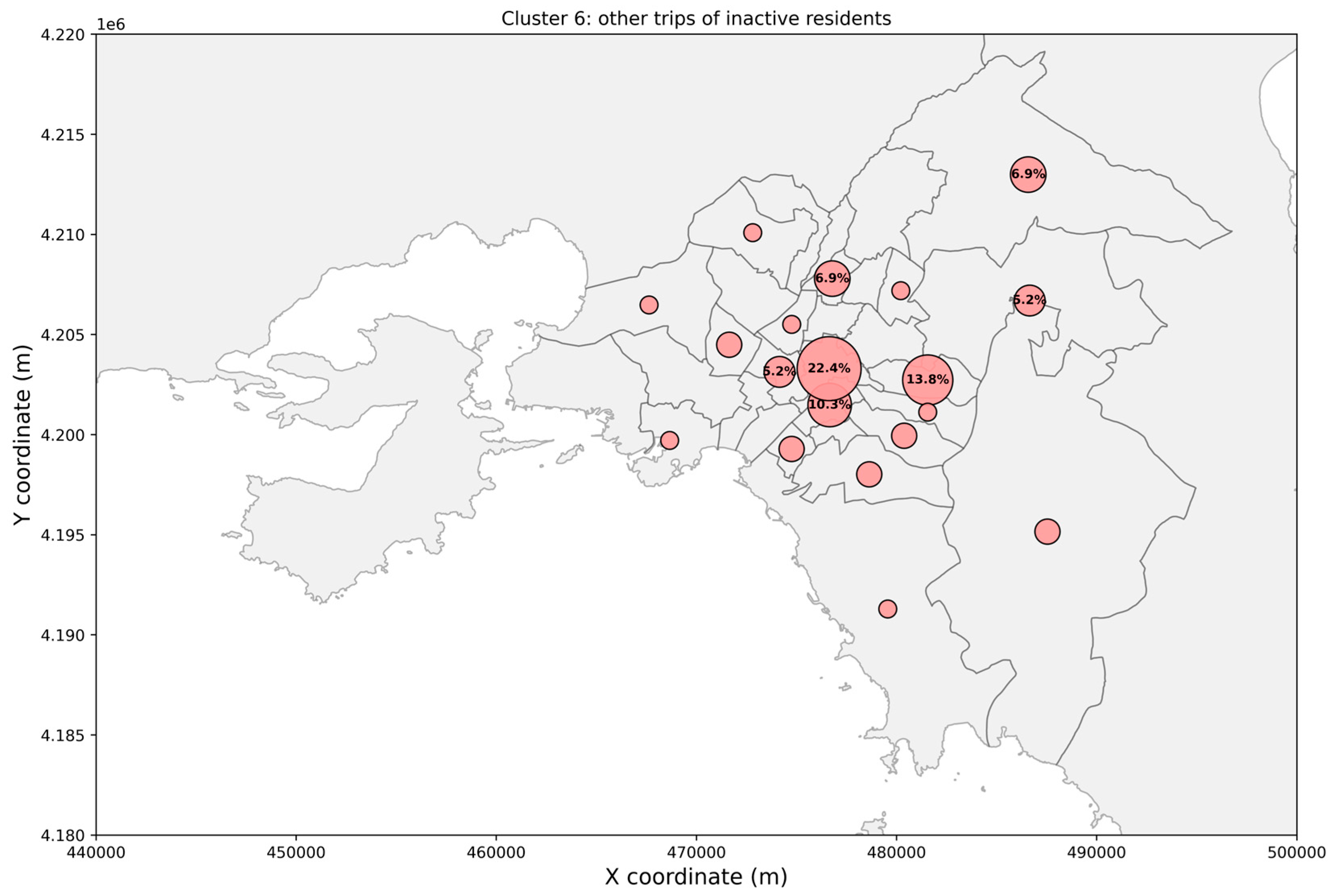
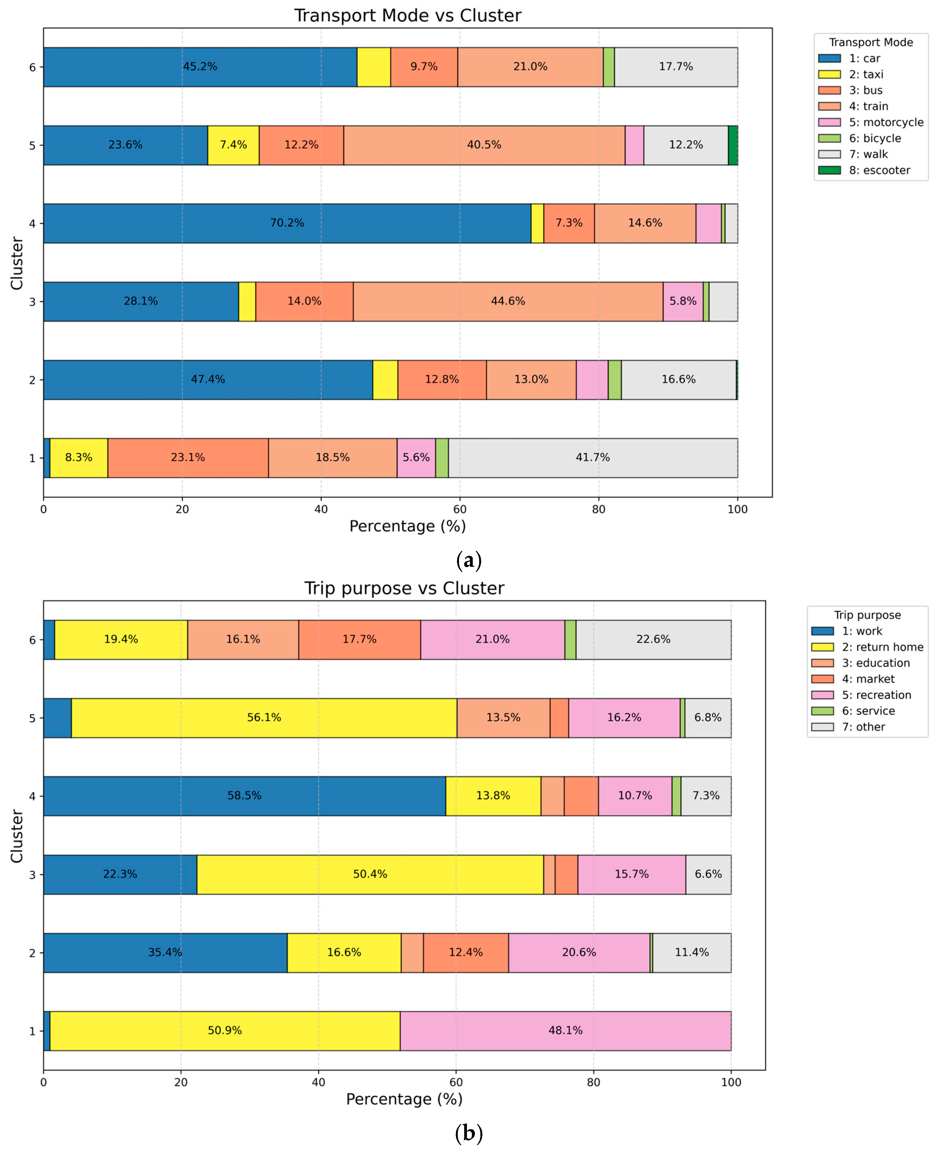
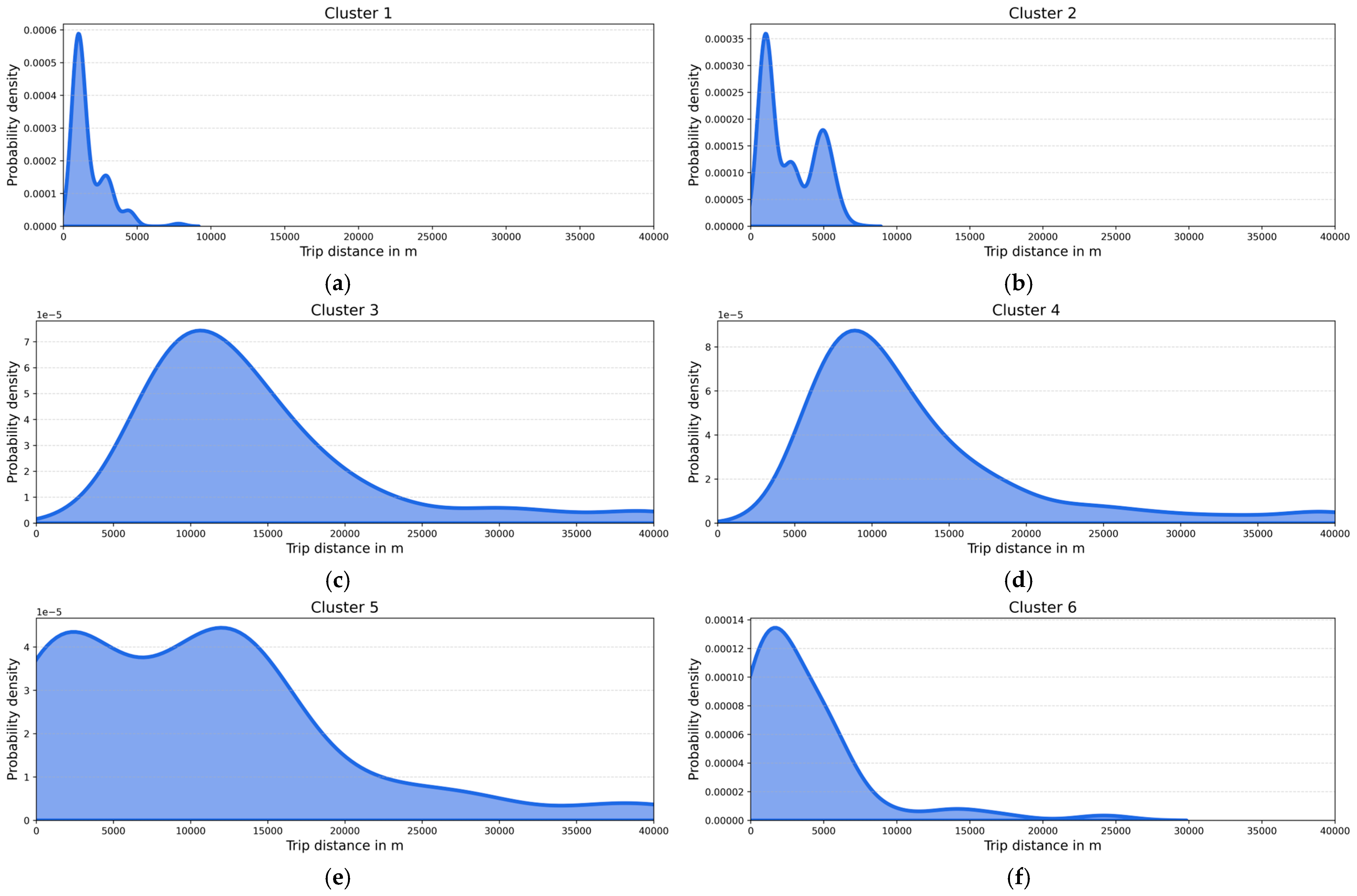
| Cluster | Preferred Transport Modes | Mean Trip Distance (Std. Dev) | Departure Time Period, 75% of Trips | Main Trip Purposes |
|---|---|---|---|---|
| Cluster 1 | Walking (41.7%) | 1.68 km (±1.17) | 16:00–22:00 | Home (50.9%) |
| Bus (23.1%) | Recreation (48.1%) | |||
| Cluster 2 | Car (47.4%) | 2.70 km (±1.82) | 07:00–11:00 | Work (35.4%) |
| Walking (16.6%) | Recreation (20.6%) | |||
| Cluster 3 | Train (44.6%) | 14.04 km (±7.46) | 07:00–20:00 | Home (50.4%) |
| Car (28.1%) | Work (22.3%) | |||
| Cluster 4 | Car (70.2%) | 12.95 km (±7.67) | 06:00–17:00 | Work (58.5%) |
| Train (14.6%) | Home (13.8%) | |||
| Cluster 5 | Train (40.5%) | 10.60 km (±9.35) | 00:00–12:00 | Home (56.1%) |
| Car (23.6%) | Recreation (16.2%) | |||
| Cluster 6 | Car (45.2%) | 3.67 km (±4.30) | 08:00–12:00 | Other (22.6%) |
| Train (21.0%) | Recreation (21.0%) |
| The Trip “Owner” Is/Has: | Cluster 1 | Cluster 2 | Cluster 3 | Cluster 4 | Cluster 5 | Cluster 6 |
|---|---|---|---|---|---|---|
| Female | 59 | 337 | 77 | 217 | 84 | 35 |
| Male | 47 (p: 0.250) | 189 (p: 0.016) | 46 (p: 0.618) | 164 (p: 0.160) | 65 (p: 0.401) | 27 (p: 0.816) |
| 18–30 years | 50 (p: 1.000) | 233 (p: 0.185) | 63 (p: 0.160) | 167 (p: 0.327) | 90 (p: <0.001) | 23 (p: 0.078) |
| 31–40 years | 32 (p: 0.051) | 116 (p: 0.755) | 18 (p: 0.042) | 92 (p: 0.293) | 27 (p: 0.229) | 11 (p: 0.347) |
| 40–50 years | 11 (p: 0.094) | 71 (p: 0.129) | 27 (p: 0.034) | 74 (p: 0.012) | 20 (p: 0.605) | 5 (p: 0.150) |
| 50–65 years | 12 (p: 0.371) | 101 (p: 0.000) | 13 (p: 0.277) | 43 (p: 0.026) | 9 (p: 0.003) | 17 (p: <0.001) |
| >65 years | 3 (p: 0.579) | 4 (p: 0.021) | 1 (p: 0.367) | 4 (p: 0.964) | 3 (p: 1.000) | 7 (p: <0.001) |
| Primary School graduate | 0 | 0 | 1 (p: 0.428) | 0 | 0 | 0 |
| High School gradute | 22 (p: 1.000) | 98 (p: 0.340) | 27 (p: 0.518) | 50 (p: 0.000) | 50 (p: 0.000) | 22 (p: 0.002) |
| Bachelor graduate | 42 (p: 0.896) | 221 (p: 0.217) | 50 (p: 0.673) | 156 (p: 0.755) | 48 (p: 0.059) | 20 (p: 0.258) |
| Master/PhD graduate | 46 (p: 0.767) | 207 (p: 0.749) | 42 (p: 0.264) | 175 (p: 0.007) | 50 (p: 0.091) | 20 (p: 0.263) |
| Inactive | 5 (p: 0.767) | 26 (p: 0.749) | 1 (p: 0.264) | 9 (p: 0.007) | 3 (p: 0.091) | 16 (p: 0.263) |
| Unemployed | 5 (p: 0.737) | 7 (p: 0.763) | 22 (p: 0.072) | 4 (p: 0.027) | 5 (p: 0.192) | 1 (p: <0.001) |
| Student | 22 (p: 0.005) | 80 (p: 0.528) | 98 (p: 0.249) | 39 (p: 0.342) | 46 (p: 0.185) | 12 (p: 1.000) |
| Active | 72 (p: 0.212) | 411 (p: 0.335) | 9 (p: 0.707) | 330 (p: 0.000) | 92 (p: 0.000) | 32 (p: 0.434) |
| 0 euros income | 19 (p: 0.232) | 63 (p: 0.718) | 15 (p: 1.000) | 34 (p: 0.012) | 28 (p: 0.028) | 12 (p: 0.192) |
| <750 euros income | 22 (p: 1.000) | 102 (p: 0.798) | 26 (p: 0.939) | 65 (p: 0.129) | 42 (p: 0.011) | 12 (p: 1.000) |
| 750–1500 euros income | 51 (p: 0.789) | 269 (p: 0.211) | 53 (p: 0.421) | 194 (p: 0.442) | 55 (p: 0.007) | 34 (p: 0.365) |
| 1500–2500 euros income | 15 (p: 0.634) | 96 (p: 0.170) | 20 (p: 0.925) | 69 (p: 0.392) | 15 (p: 0.060) | 4 (p: 0.081) |
| >2500 euros income | 4 (p: 0.497) | 5 (p: 0.014) | 3 (p: 1.000) | 16 (p: 0.022) | 4 (p: 0.956) | 0 (p: 0.422) |
| not car owner | 26 | 92 | 26 | 30 | 35 | 0 |
| car owner | 82 (p: 0.027) | 433 (p: 0.293) | 95 (p: 0.119) | 353 (p: 0.000) | 113 (p: 0.012) | 54 (p: 0.599) |
Disclaimer/Publisher’s Note: The statements, opinions and data contained in all publications are solely those of the individual author(s) and contributor(s) and not of MDPI and/or the editor(s). MDPI and/or the editor(s) disclaim responsibility for any injury to people or property resulting from any ideas, methods, instructions or products referred to in the content. |
© 2025 by the authors. Licensee MDPI, Basel, Switzerland. This article is an open access article distributed under the terms and conditions of the Creative Commons Attribution (CC BY) license (https://creativecommons.org/licenses/by/4.0/).
Share and Cite
Andrinopoulou, E.; Tzouras, P.G. Applying Spectral Clustering to Decode Mobility Patterns in Athens, Greece. Appl. Sci. 2025, 15, 3419. https://doi.org/10.3390/app15073419
Andrinopoulou E, Tzouras PG. Applying Spectral Clustering to Decode Mobility Patterns in Athens, Greece. Applied Sciences. 2025; 15(7):3419. https://doi.org/10.3390/app15073419
Chicago/Turabian StyleAndrinopoulou, Eirini, and Panagiotis G. Tzouras. 2025. "Applying Spectral Clustering to Decode Mobility Patterns in Athens, Greece" Applied Sciences 15, no. 7: 3419. https://doi.org/10.3390/app15073419
APA StyleAndrinopoulou, E., & Tzouras, P. G. (2025). Applying Spectral Clustering to Decode Mobility Patterns in Athens, Greece. Applied Sciences, 15(7), 3419. https://doi.org/10.3390/app15073419