Real-Time Elbow and T-Junction Detection and Estimation Framework for In-Line Inspection in Natural Gas Pipelines Using 3D Point Cloud

Abstract

In-line inspection (ILI) is essential for maintaining the integrity of natural gas pipelines. In ILI, pipeline inspection gauges (PIGs) autonomously navigate through pipelines under real-time and resource-constrained conditions to measure pipeline irregularities. Elbow and T-junction detection and estimation (ETDE) play a critical role in enabling PIG navigation to avoid speed excursions which prevent effective data collection or even damage the PIG and pipelines. Existing approaches are often computationally intensive, incomplete, or late estimations, making them unsuitable for real-time operation in such environments. This paper proposes a real-time elbow and T-junction detection and estimation (RT-ETDE) framework that efficiently detects elbows and T-junctions and estimates their critical parameters for PIG navigation using 3D point clouds. Our framework relies on intelligent point cloud partition and feature extraction together with simple geometric solutions which greatly reduce computational complexity. Furthermore, several real-time adaptation techniques are introduced to ensure real-time operation. Experimental results on a prototype pipeline demonstrate that the RT-ETDE framework consistently detects elbows and T-junctions while achieving a 10 Hz frame rate on a real PIG processing unit, validating its suitability for next-generation pipeline inspection systems.

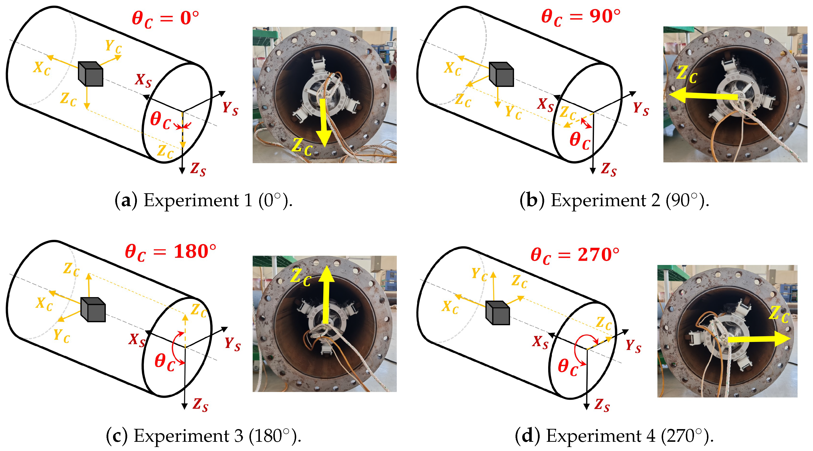
1. Introduction

In-line inspection (ILI) plays a crucial role in pipeline management, ensuring the safety and reliability of natural gas pipelines. A pipeline inspection gauge (PIG) is a device widely used in ILI to measure irregularities in the pipe, including corrosion, cracks, and deformations [1,2,3]. In natural gas pipelines, a PIG is passively moved by the pressure of the gas flow over hundreds of kilometers, carrying various sensors, including magnetic, acoustic, optical, etc. For efficient data collection, a PIG is required to move at a stable speed. However, features such as elbows, T-junctions, significant thickness changes, or heavy welds can cause a PIG device to become stuck. Once the pressure builds up behind a PIG device, it can result in sudden speed surges reaching tens of meters per second [4,5]. This phenomenon, known as speed excursion, not only prevents the sensors from fully collecting data but also incurs damage to PIGs and pipelines. In lower-pressure pipelines, the speed excursion is even more severe, making them nearly impossible for PIG operation. To address this problem, newer PIG systems are equipped with advanced mechanisms like pressure controls and active joints to regulate the speed to smoothly move through elbows, T-junctions, significant thickness changes, or heavy welds. Detecting and estimating these features along the pipeline plays a key role in the success of these control mechanisms. While significant thickness change and heavy welds need adaptive pressure controls, elbows and T-junctions require much more complicated control maneuvers involving both pressure controls and active joints. This paper focuses on elbow and T-junction detection and estimation (ETDE).

The ETDE problem involves detecting elbows and T-junctions as well as estimating their critical parameters to enable PIG devices to navigate through these features smoothly. For elbows, these parameters consist of the distance to the elbow, its direction, radius, and length. Similarly, T-junction parameters include the distance to the T-junction, the direction of its branch, the branch radius, and the length of the T-junction. To be integrated into PIG systems, ETDE must address two key constraints: limited processing power and real-time operation. ETDE is performed on the PIG processing unit with limited processing power due to the limited battery and long operating distance. It also needs to perform ETDE in real-time to promptly react to the existence of elbows and T-junctions. These conflicting constraints present significant challenges to the ETDE problem. Given these constraints, ETDE needs to provide early and reliable detection to support maneuvering in high-speed movement while achieving reasonable accuracy.

The existing approaches for ETDE rely on either contact sensors [6,7], 2D cameras [8,9,10,11], stereo camera [12,13], or 3D ranging sensors [14,15]. While contact sensors approaches [6,7] offer low-complexity solutions, they are unsuitable for PIGs due to delayed detection and the potential for PIG and pipe damage at high speeds. On the other hand, cameras [8,9,10,11] and stereo 2D cameras [12,13] suffer from inherently high complexity due to image processing. The 3D ranging sensors are a promising approach for ETDE in PIG systems. However, the existing approach [14,15] requires high computation power for processing the entire point cloud, making them impractical under real-time and resource-constrained conditions. To overcome these challenges, ETDE solutions must be carefully designed and optimized to account for the unique geometric characteristics of elbows and T-junctions, ensuring both computational efficiency and real-time performance.

In this paper, we propose a real-time elbow and T-junction detection and estimation (RT-ETDE) framework, designed to address the challenges of computational efficiency and real-time processing in PIG systems. The RT-ETDE framework consists of a set of lightweight schemes for ETDE that rely on intelligent point cloud partition, feature extraction, and simple geometric solutions based on the characteristics of the point cloud in elbows and T-junctions. We present a linear-time sampling scheme for the camera pose and straight pipe diameter estimation. The elbow and T-junction are detected by evaluating the coverage of the point cloud in the inner and outer area from the straight pipe. The elbow direction is estimated by the deviation direction of the cloud, while the elbow radius and distance are computed via the estimation of its tangent. The elbow length is estimated by detecting the deviation of the point cloud from the elbow model. On the other hand, the branch direction of the T-junction is computed by identifying the highest intensity area. The branch radius is estimated based on the circumcircle through three points on the branch, while the T-junction distance and length are directly inferred from these points. To ensure real-time operation, several techniques are applied, including point skipping, language-dependent optimizations, and a multi-processor offloading scheme to distribute computational tasks across processors in the real PIG processing unit. The results collected with the pull-rig robot and the prototype pipeline validate that the RT-ETDE framework consistently detects and estimates the elbow and T-junction, as well as satisfying real-time constraints with a 10 Hz frame rate on the real PIG processing unit. The contribution of this paper is summarized as follows:

• We propose an RT-ETDE framework which is the first solution that simultaneously achieves real-time operation, early detection, and full parameter estimation of elbows and T-junctions using 3D point clouds.
• We propose a set of schemes for detecting and estimating each parameter of elbows and T-junctions in the RT-ETDE framework. Each scheme is designed to be computationally efficient and robust by relying on intelligent point cloud partition, feature extraction, and simple geometric solutions.
• We present several techniques, including a multi-processor offloading scheme, to ensure the real-time constraint.
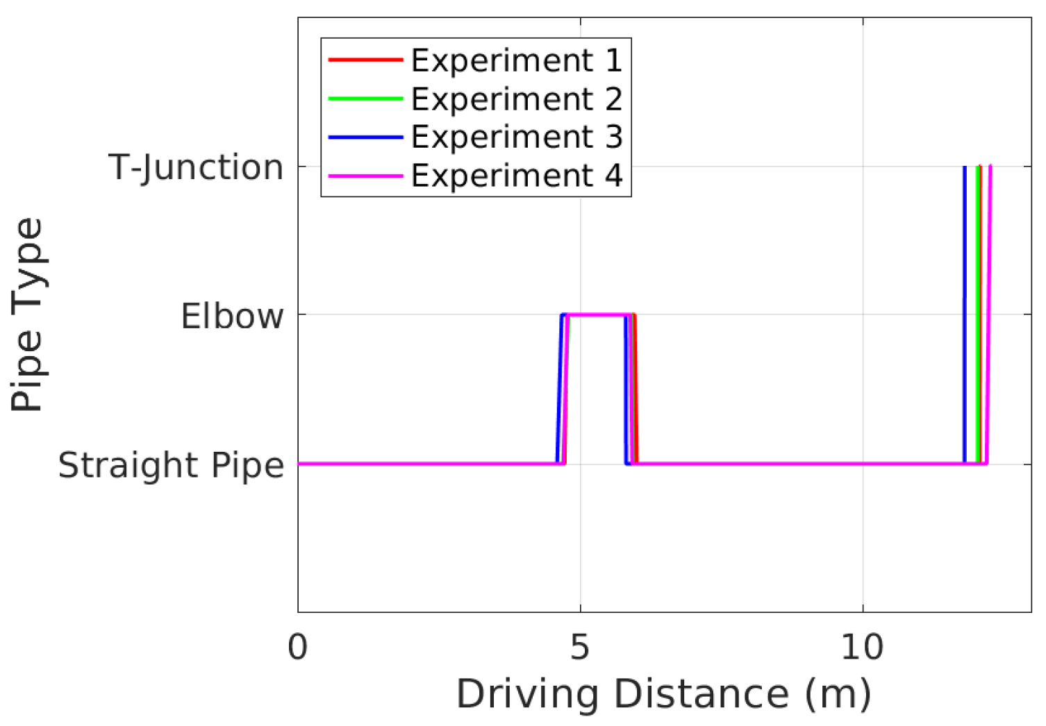
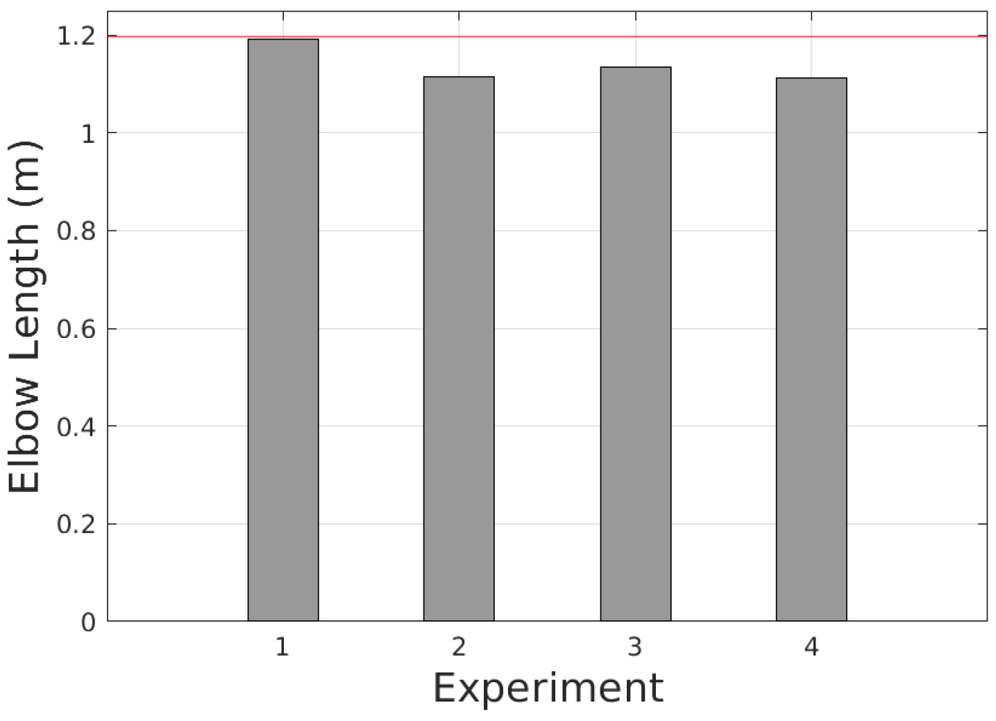
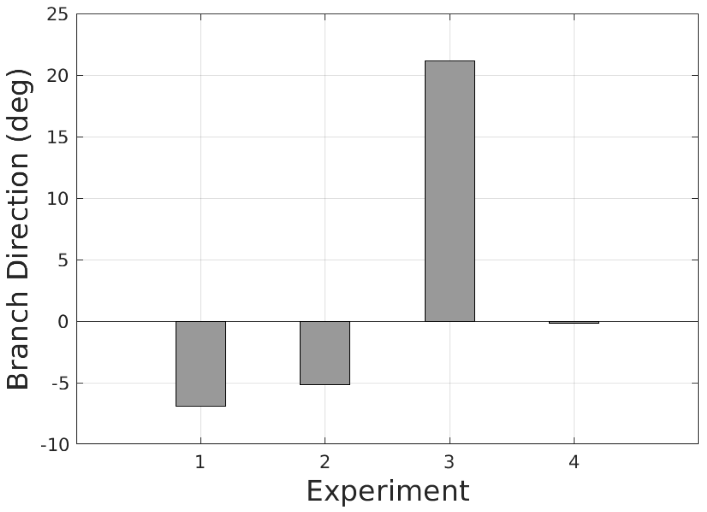
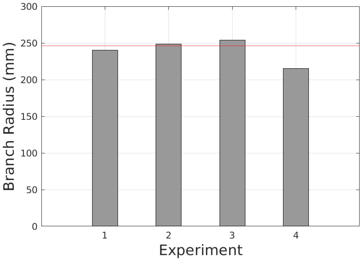
• We validate the performance of the framework with real experiments. The results show that the detection and estimation are consistent.
• The processing time result on the real PIG processing unit indicates that the RT-ETDE framework satisfies the 10-Hz real-time constraint.

The remainder of this paper is organized as follows. Section 2 introduces related works. Section 3 describes the system model and defines the problem. In Section 4, we present our RT-ETDE framework. The real-time adaptation techniques are presented in Section 5. The numerical results are discussed in Section 6, and finally, the conclusion of this paper is given in Section 7.

2. Related Works

ETDE under limited processing power and real-time constraints is critical for modern PIG control systems in natural gas pipelines. Existing methods for ETDE are primarily designed for short pipelines or slower-moving, non-isolated robots, where these constraints are less critical. These approaches can be categorized based on the sensors used: contact sensors [6,7], 2D cameras [8,9,10,11], stereo cameras [12,13], and 3D ranging sensors [14,15]. They are summarized in

Table 1. Comparison of elbow and T-junction detection and estimation approaches.

Approach	Sensor	Feature	Detection Approach	Estimation Parameter	Estimation Approach
[6]	Contact	Elbow	Deviation of contact sensors	Direction	Deviation of center point
[7]	Contact	Elbow	Deviation of contact sensors	Direction	Angle of two most deviated sensors
[8]	2D Camera	Elbow and T-junction	Edge detection and pattern matching	No estimation	No estimation
[9]	2D Camera	Elbow and T-junction	Image classification based on deep learning	No estimation	No estimation
[10]	2D Camera	Elbow and T-junction	Edge detection and pattern matching	Direction	Direction of pattern
[11]	2D Camera	Elbow	Edge detection and pattern matching	Direction	Distortion of pattern
[12]	Stereo Camera	Elbow and T-junction	Edge detection and pattern matching	Distance	Stereo matching
[13]	Stereo Camera	Elbow and T-junction	Edge detection and pattern matching	Distance	Stereo matching and laser profiler
[14]	Pseudo 3D LIDAR	Elbow and T-junction	Outlier detection of straight pipe and circle fitting	Elbow direction and radius	Circle fitting
[15]	3D ToF Camera	Elbow and T-junction	Outlier detection of straight pipe by blob grouping	Distance	Position of blob
RT-ETDE	3D ToF Camera	Elbow and T-junction	Outlier detection of straight pipe by point cloud partition and simple feature extraction	Full parameters	Point cloud partition, simple feature extraction, and simple geometric solutions.

.

The first approach involves attaching contact sensors to the front of the robot to detect elbows and T-junctions by physically interacting with the inner pipe surface. In [6], three contact sensors are evenly placed circumferentially to detect elbows by observing deviations in the center point of the contact points. Consecutive center points are aggregated to estimate the direction and radius of the elbow. Similarly, ref. [7] uses four contact sensors to detect elbows, where the direction and position are computed from the two most deviated sensors. Because of their simplicity in processing, these approaches are ideal for the limited processing power and real-time systems in general. However, they are unsuitable for PIG in natural gas pipelines since they detect features only after partial entry into the elbow, limiting reaction time for the control system. Moreover, at high speeds, contact sensors risk damaging both the pipelines and themselves.

The second approach employs a single 2D camera to detect the elbow and T-junction. In [8], a camera paired with an LED illuminator is used to detect elbows and T-junctions by analyzing high-reflection areas caused by small incident angles at the elbows and T-junctions. The location and shape of these areas in the image are directly inputted to a fuzzy logic control algorithm. To improve the accuracy regarding lighting variations, a deep learning technique based on convolutional neural networks is introduced in [9] to detect elbows and T-junctions from 2D camera images. In [10], a rotating line-shaped laser paired with a 2D camera generates consecutive images to form a full scan of the pipe. The elbow and T-junction create a gap area in the scanning image. By analyzing the shape and position of this gap area, the elbow and T-junction can be detected, and their direction is also estimated. The approach in [11] uses a camera paired with four circle-and-dot laser pointers to detect the elbow. The circle and dot can only be seen in the image if an elbow exists in front of the robot. The direction and distance to the elbow can be inferred by comparing the distortion pattern of circles and dots to known patterns. These approaches rely on image processing which is of high computational complexity and opposed to the PIG constraints. Additionally, relying on the deformation of a pattern which is abstract information leads to late detection and partial parameter estimation with low granularity.

The third approach involves a stereo camera. In [12], the existence of T-junction is detected by edge detection using one camera of the stereo camera while stereo matching between both cameras of the stereo camera is performed to find the distance. However, the detection and distance measurement with the stereo camera is not accurate in the pipeline environment due to unclear features on the pipe wall. To address this issue, the approach in [13] additionally uses the second distance measurement mechanism using a rotating laser profiler. When the robot is close to the T-junction detected by the stereo camera, the highly accurate laser profiler is activated to detect and measure the distance to it. These approaches share the same computational complexity issues with the 2D camera.

The fourth approach utilizes 3D ranging sensors. In [14], a pseudo-3D ranging sensor using a rotating 2D LIDAR detects elbows and T-junctions by recognizing outlier points inside or outside the straight pipe. The direction and radius of elbows are estimated by fitting circles to LIDAR data at various angles, but this scheme depends heavily on accurate calibration and is sensitive to misalignment, limiting its reliability at longer distances. 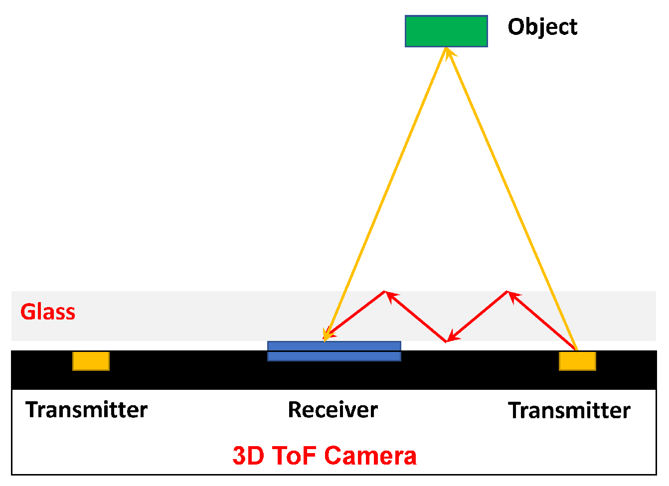In [15], a 3D time-of-flight (ToF) camera is employed to model the straight pipe and identify outlier points. These points are grouped into blobs, with gradients analyzed to distinguish between elbows and T-junctions. However, both approaches require processing the entire point cloud, resulting in excessive computational complexity.

The fourth approach utilizes 3D ranging sensors to detect and estimate the elbow and T-junction. In [14], a pseudo-3D ranging sensor created by rotating a 2D LIDAR is equipped in front of the robot. The elbow and T-junction are detected by recognizing the existence of points inside or outside of the straight pipe, respectively. Additionally, to estimate the direction and radius of the elbow, 2D LIDAR data at each rotating angle are fitted with the circle, and the rotating angle with the smallest fitting error indicates the direction of the elbow. However, the rotation mechanism requires multiple frame processing and careful calibration. Additionally, the elbow direction and radius estimation are sensitive to misalignment of the robot inside the pipe and only effective at close distances. The 3D ToF camera is a solution for these multiple frame issues in [15]. The measured points are first used for fitting to find the circular cylinder model of the straight pipe. Then, the measurement points that are outlier points from the straight pipe model are considered candidate regions. They are first grouped into blobs of connected pixels. Gradients of points inside a blob and between blobs are used to evaluate the shape change inside a blob and between blobs, respectively. Blobs with small shape change internally and big changes to the other shapes are considered to be elbows or T-junctions. Only the distance to these features is estimated in this work. In general, both approaches in [14,15] rely on the processing of entire measurement points, which is high in computational complexity.

The existing approaches share three common issues when considering their application to PIG systems, including the following: (1) excessive processing complexity for real-time and resource-constrained systems, (2) late detection leaving insufficient time for corrective maneuvers, and (3) incomplete estimation of parameters. In this paper, we address these issues by proposing the RT-ETDE framework using a 3D ToF camera that consists of a set of lightweight schemes for ETDE. Unlike [14,15], RT-ETDE does not use the whole point cloud for detection and estimation but intelligently partitions the point cloud into groups and extracts only simple representative features, such as centroid, extreme point, or the number of points, to apply simple geometric solutions. Additionally, we propose several real-time adaptation techniques to ensure the real-time constraint. This is the first work that supports early detection and full parameter estimation of elbows and T-junctions in real time.

3. Preliminaries

3.1. System Model

The PIG is equipped with a 3D ToF camera and other inspection sensors, such as magnetic, acoustic, optical, etc. In this paper, we only focus on the 3D ToF camera for ETDE. The 3D ToF camera is placed in front of the PIG. The 3D ToF camera has a resolution of $N_H\times N_W$ and covers a view $F_H\times F_W$. The 3D ToF camera coordinate system is illustrated in Figure 1 where the origin $O_C$ is defined in the center of the lens and $X_C$, $Y_C$, and $Z_C$ axes point to the forward, leftward, and downward directions of the 3D ToF camera, respectively. At each time step, it creates a point cloud with $N_H\times N_W$ points representing the inner surface of the pipeline ahead of the PIG. Each point in the point cloud has the form of $(x_C, y_C, z_C, I)$ where $(x_C, y_C, z_C)$ is the coordinate in the camera coordinate system and I is the intensity value.

We consider the PIG that operates in the gas pipelines consisting of straight pipes, elbows, and T-junctions. The straight pipe is assumed to have an elliptic cylinder shape. The straight pipe coordinate system (SCS) is defined as follows: the origin $O_S$ is the intersection pipe central axis and the start cross-section, $X_S$ axis is along the central axis and points toward the moving direction of PIG, $Z_S$ axis follows the direction of gravity, and $Y_S$ axis is defined according to the right-hand rule, as shown in Figure 1.

The elbow is designed as a section of the torus shape [16] with radius $R_E$ and pipe radius $r_E$, as shown in Figure 2. The elbow coordinate system is defined as follows. The origin $O_E$ is the center of the torus shape. $X_E$ axis is assumed to be parallel and same direction as $X_S$ of SCS. $X_E$ and $Y_E$ axes define the elbow plane and $Y_E$ axis points to the direction of the elbow. Note that $X_S$ is also on the elbow plane. $Z_E$ axis is defined according to the right-hand rule. $S_E$ is the starting point of the elbow from the straight pipe and $E_E$ is the ending point of the elbow, which is also the starting point of the subsequent straight pipe. The length $l_E$ of the arc between $S_E$ and $E_E$ represents the elbow length.

The T-junction’s design is shown in Figure 3a with the main pipe radius $r_T$ and branch radius $r_B$. It can be a smooth T-junction or shaft T-junction, as shown in Figure 3b,c. While the smooth T-junction is a distinct part of the pipeline, the shaft T-junction is created by hot-tapping the branch to the existing straight pipe. In both types, the T-junction coordinate system is defined as follows. $X_T$ axis is also aligned with the straight pipe $X_S$ while the $Y_T$ axis points to the direction of the branch. $Z_T$ axis is derived using the right-hand rule. Note that, in reality, the PIG only moves in the main pipe of the T-junction, as shown in Figure 3a. To make a consistent definition among two types of T-junction, we define the start point $O_T$ and end point $E_T$ of the T-junction as the point on the central axis and aligning with the branch’s inner wall, as shown in Figure 3b,c. The starting point $O_T$ is also defined as the origin. The distance from $O_T$ and $E_T$ defines the T-junction length $l_T$.

3.2. Problem Definition

The PIG is required to detect the existence of the elbow and T-junction, as well as accurately estimate their parameters given the limited processing power and real-time constraint. For the estimation of elbow parameters, since the $X_E$ is aligned with $X_S$, we only need to estimate the direction represented by ${\theta }_E$, elbow radius $R_E$, distance from the camera $\Delta x_E$, and elbow length $l_E$ to define the elbow, as shown in Figure 2. For the estimation of T-junction parameters, the direction ${\theta }_T$, the branch radius $r_B$, the distance from the camera $\Delta x_T$, and T-junction length $l_T$ are needed to define the T-junction, as shown in Figure 3a. Here, we assume that the elbow pipe radius $r_E$ and T-junction main pipe radius $r_T$ are equal to the straight pipe radius. Note that, if they are significantly different, the thickness change estimation should be used and is out of the scope of this paper.

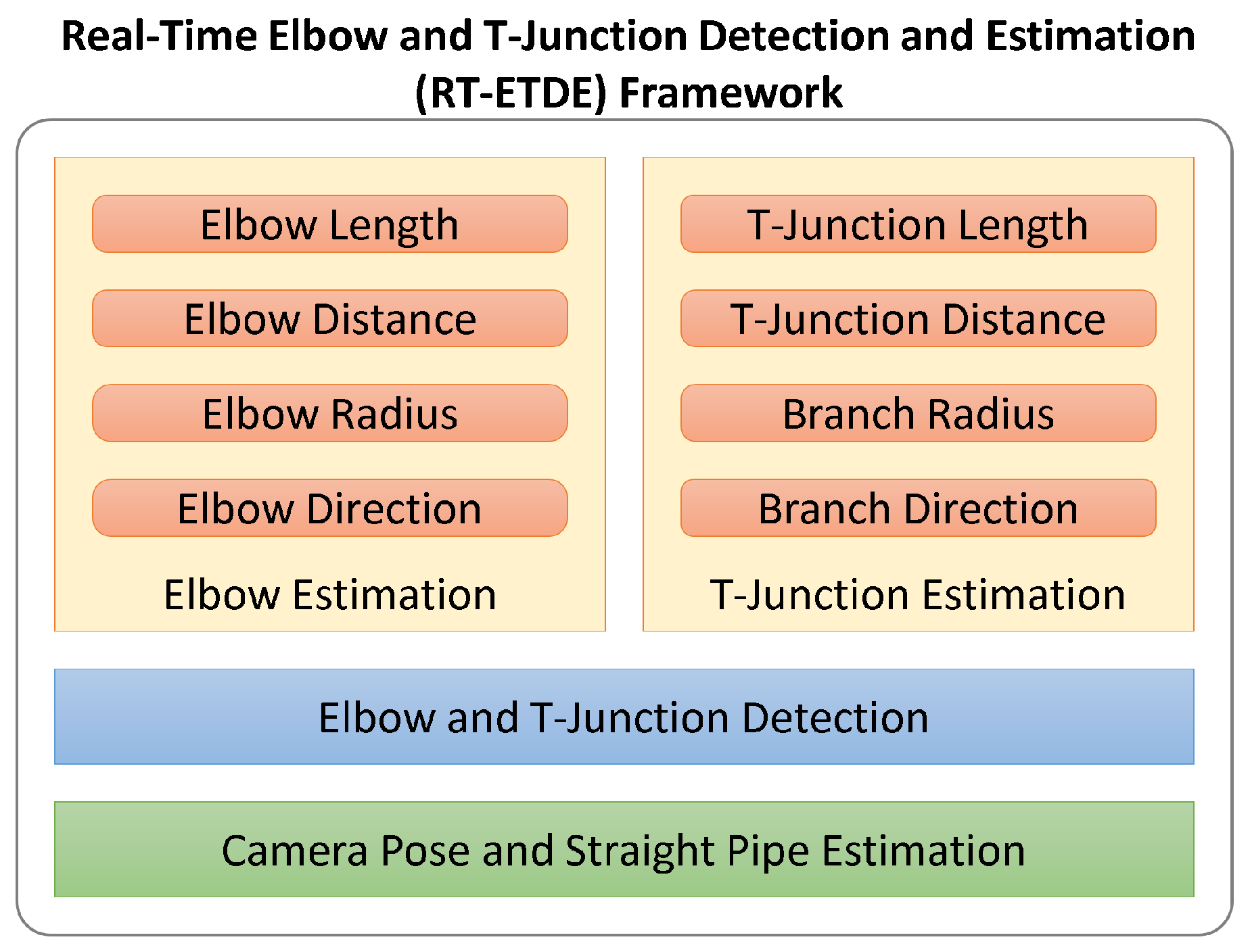
4. Real-Time Elbow and T-Junction Detection and Estimation (RT-ETDE) Framework

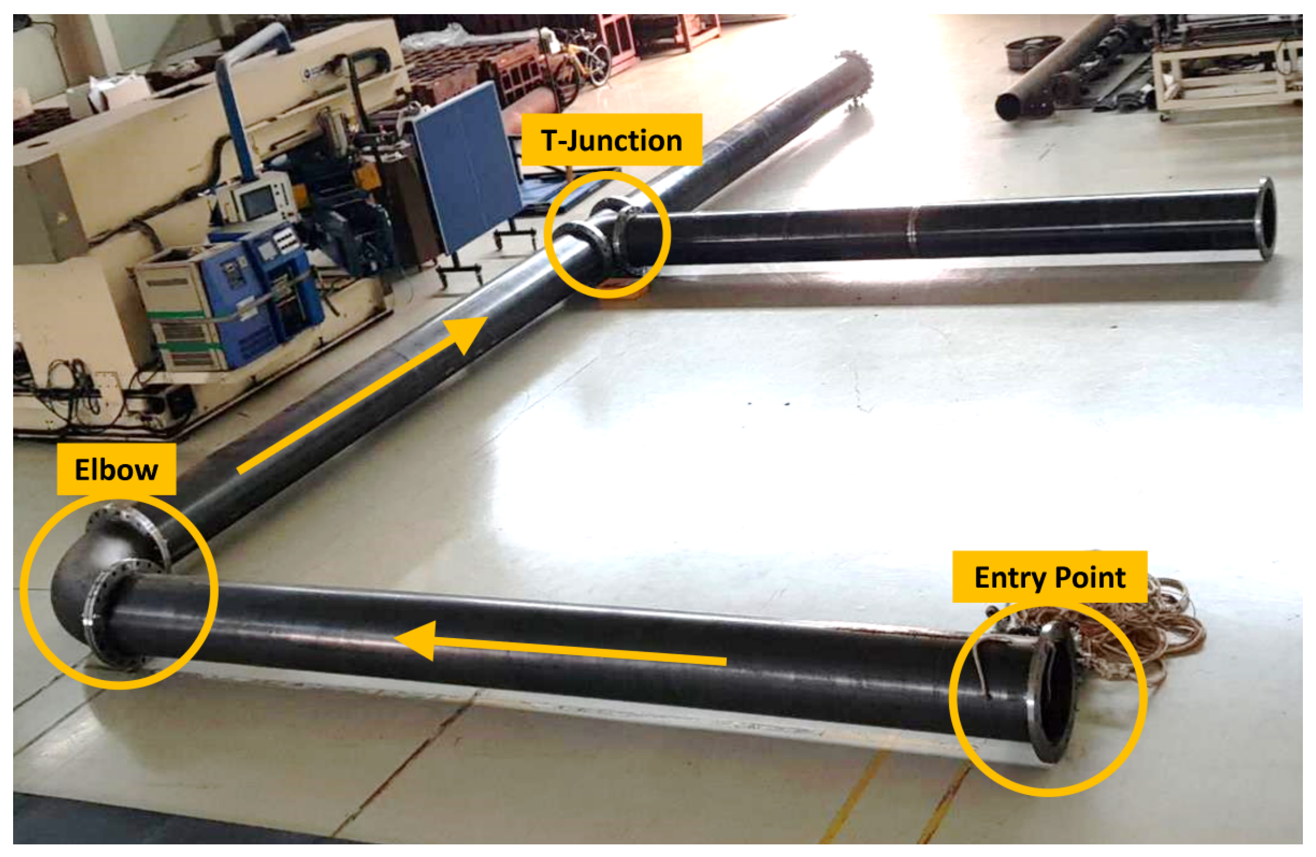
In this section, we propose the real-time elbow and T-junction detection and estimation (RT-ETDE) framework consisting of four blocks, as shown in Figure 4. The first block estimates the camera pose in SCS and the straight pipe model. It enables the transformation of the camera point cloud to SCS and the identification of points on the straight pipe. The second block detects the presence of the elbow and the T-junction. Upon detection, the framework activates either the elbow or T-junction estimation accordingly. When the elbow is detected, the elbow estimation estimates the elbow direction, radius, distance from the 3D ToF camera, and length. Similarly, for a T-junction, the branch direction, diameter, distance from the 3D ToF camera, and length are estimated.

4.1. Camera Pose and Straight Pipe Estimation Based on Linear-Time Point Sampling

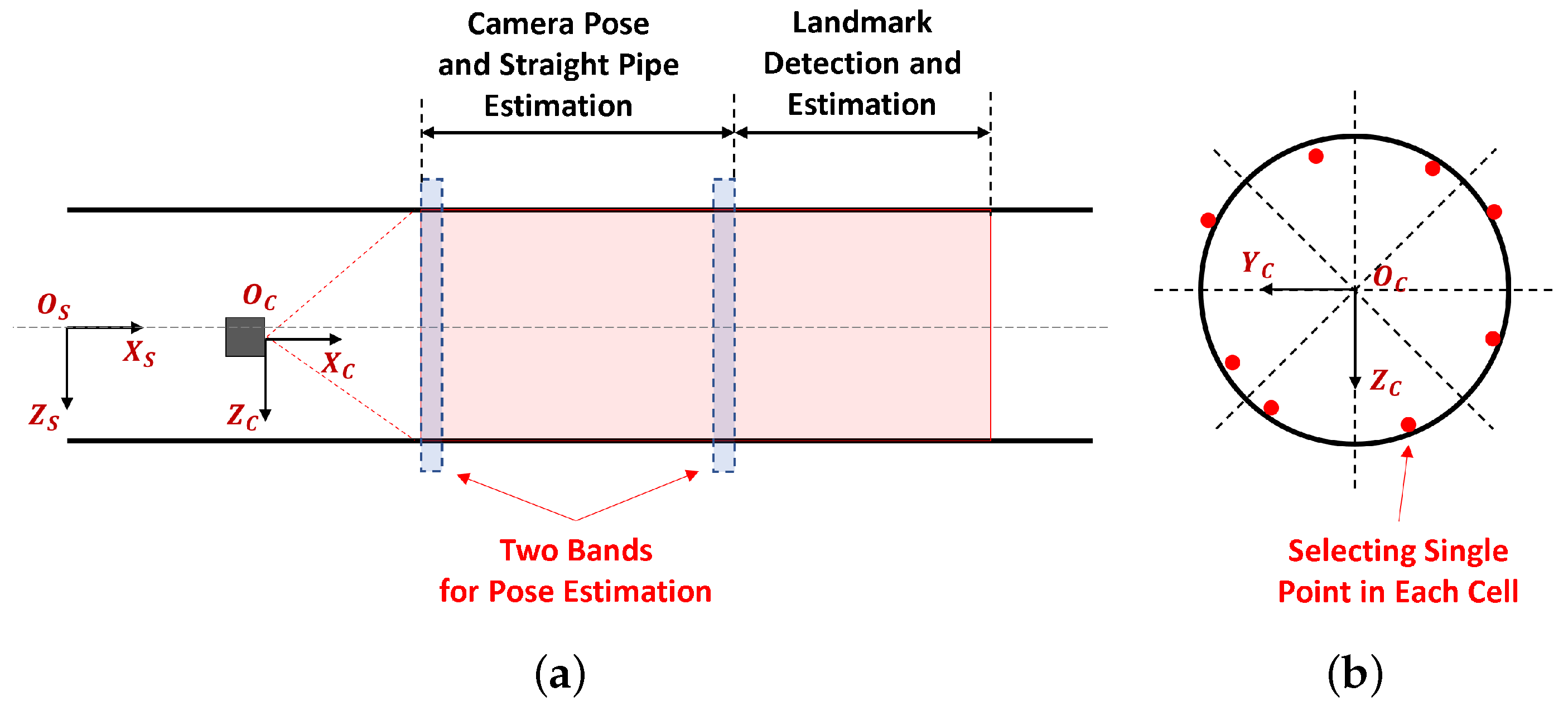
Camera pose and straight pipe estimation is an important preprocessing step in the RT-ETDE framework. Camera pose estimation in the straight pipe allows the transformation of the point cloud to SCS, which is necessary to remove the effect of the misalignment between the camera and the straight pipe. On the other hand, the straight pipe estimation provides the elliptic cylinder model of the pipe, which can be used to separate points on this pipe and points on the elbow and T-junction.

This process uses a portion of the point cloud closer to the 3D ToF camera, reserving the remainder for ETDE, as illustrated in Figure 5a. We apply the camera pose and pipe diameter estimation scheme based on the elliptic cylinder fitting in [17]. The scheme estimates the 7-tuple $\mathit{\beta }=(D_{max}, D_{min}, {\theta }_x, {\theta }_y, {\theta }_z, d_y, d_z)$ where $D_{max}, D_{min}$ are the major and minor axes of the elliptic cylinder representing the straight pipe, and ${\theta }_x, {\theta }_y, {\theta }_z, d_y, d_z$ are the camera pose in the SCS, consisting of roll, pitch, yaw, y-displacement, and z-displacement. This scheme finds the optimal pose that transforms the point cloud to SCS and fits to the elliptic cylinder represented by optimal $D_{max}$ and $D_{min}$.

The estimation scheme in [17] uses the entire point cloud for fitting, which is unsuitable for real-time operation. To address this issue, we present a linear-time point sampling scheme. Preliminary analysis revealed that for the same number of points M, the optimal point selection possesses two properties: (1) points are divided into two planes that are parallel to $Y_C{Z}_C$-plane and positioned farthest from each other, and (2) in each band, $M/2$ points are evenly distributed across circumferential angles around the pipe cross-section. However, selecting points closest to a plane and evenly distributed over circumferential angles requires sorting, which cannot be achieved in linear time. To overcome this, we present a near-optimal linear-time point sampling scheme. We expand the plane into a band with thickness ${\delta }_B$ along $X_C$, as illustrated in Figure 5a. Any point on this band is considered to belong to the plane. Then, we divide the circumferential angle into cells and select a single point in each cell, as illustrated in Figure 5b. As the M increases, points in cells converge to an even distribution around the circumferential angles. Given the bands and cells, point sampling becomes the problem of selecting the points in M cells in two bands. To minimize the processing time, we choose the first available point in each cell during a single iteration through the point cloud. The iteration is terminated as soon as M points are selected, ensuring linear-time complexity.

These sampled points are used for pose and straight pipe estimation using the scheme in [17] to find the camera pose and the straight pipe model. Based on the pose ${\theta }_x, {\theta }_y, {\theta }_z, d_y, d_z$, each point $(x_C, y_C, z_C)$ in the 3D ToF camera point cloud in the camera coordinate system is first transformed into the SCS $(x_S, y_S, z_S)$ and is ready for detection and estimation.

4.2. Elbow and T-Junction Detection Based on Outlier Extraction

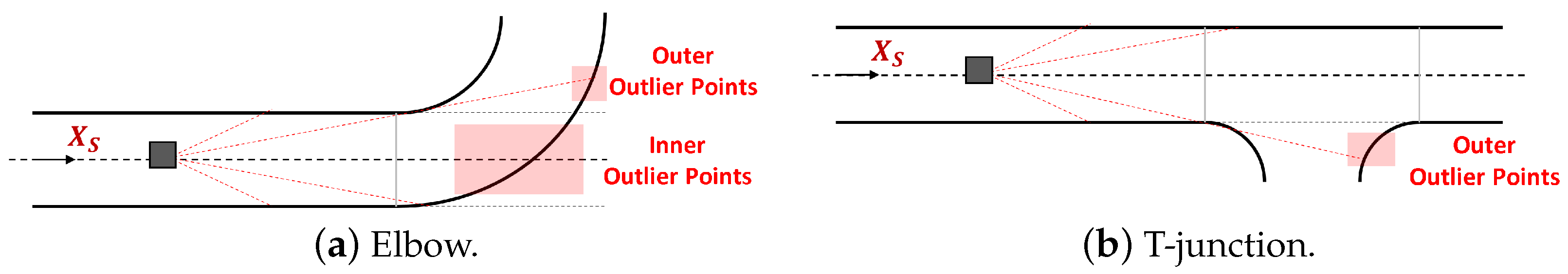
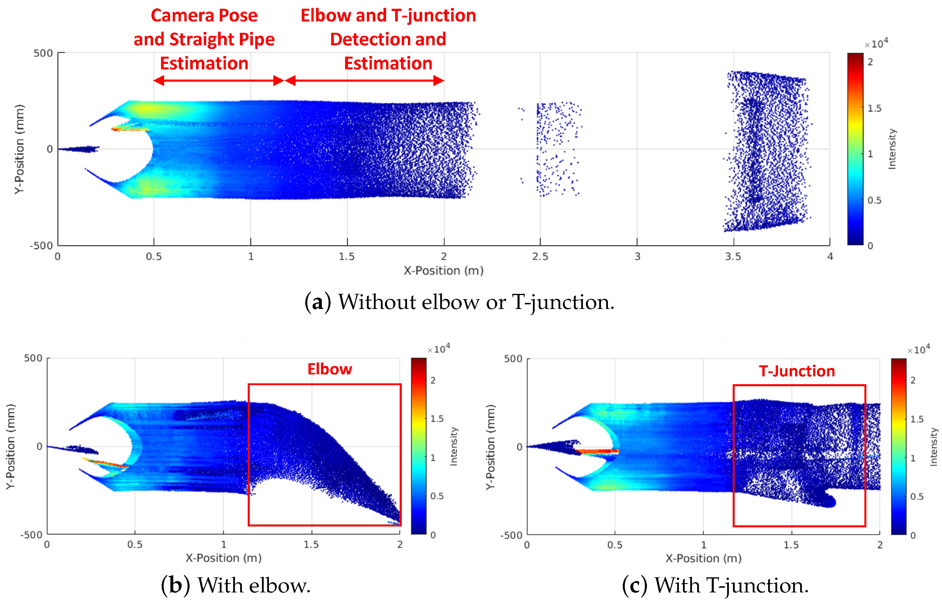
This section focuses on detecting elbows and T-junctions by analyzing outlier points that deviate from the straight pipe model within the transformed 3D point cloud in SCS. The elbow and T-junction introduce distinct patterns of outlier points, as shown in Figure 6. The elbow wall creates points in the inner and outer regions relative to the straight pipe model, which are called inner outlier points and outer outlier points, respectively. On the other hand, the branch of a T-junction only creates outer outlier points. These outlier patterns form the basis for detecting elbows and T-junctions.

To detect elbows and T-junctions, we propose a solution that relies on a simple point cloud feature. Due to multipath effects and depth errors, some outlier points may be missing, while others may not correspond to elbows or T-junctions. To address these challenges, we analyze the point coverage of inner outlier points for elbow detection and outer outlier points for T-junction detection.

We divide the point cloud into the concentric annuli in $Y_S{Z}_S$-plane with $\delta r$ difference in radius, as shown in Figure 7. By checking the number of points in each annulus exceeding a threshold or not, we can decide if the annulus contains either the elbow or T-junction. Since the inner outlier points only exist in the elbow, we first check the inner annuli to detect the elbow. If the elbow does not exist, we check the outer annuli for T-junction detection. To determine the existence of an elbow or T-junction, the number of annuli containing them should be greater than a threshold. Once detected, the parameter estimation is triggered for the elbow and T-junction accordingly.

4.3. Elbow Estimation

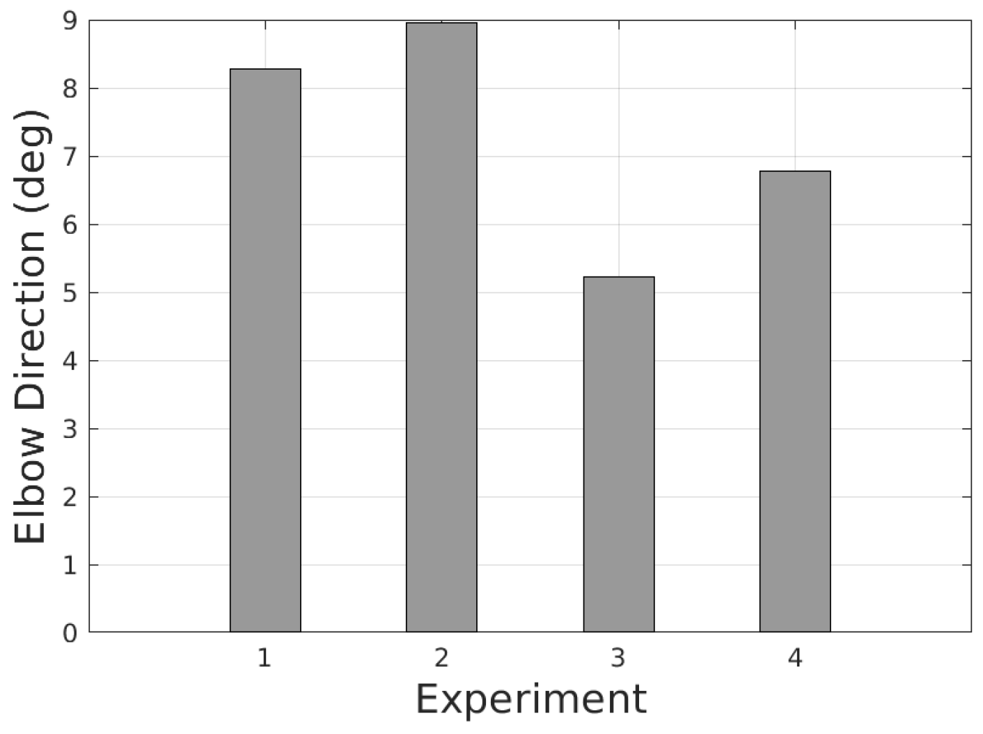
Once an elbow is detected, its critical parameters must be estimated, including direction, radius, distance from the 3D ToF camera, and length. The elbow direction determines the angle at which the PIG must turn, while the elbow radius defines the sharpness of the turn. The distance indicates the point at which the turn should begin, and the elbow length provides information on how long the turning maneuver will last.

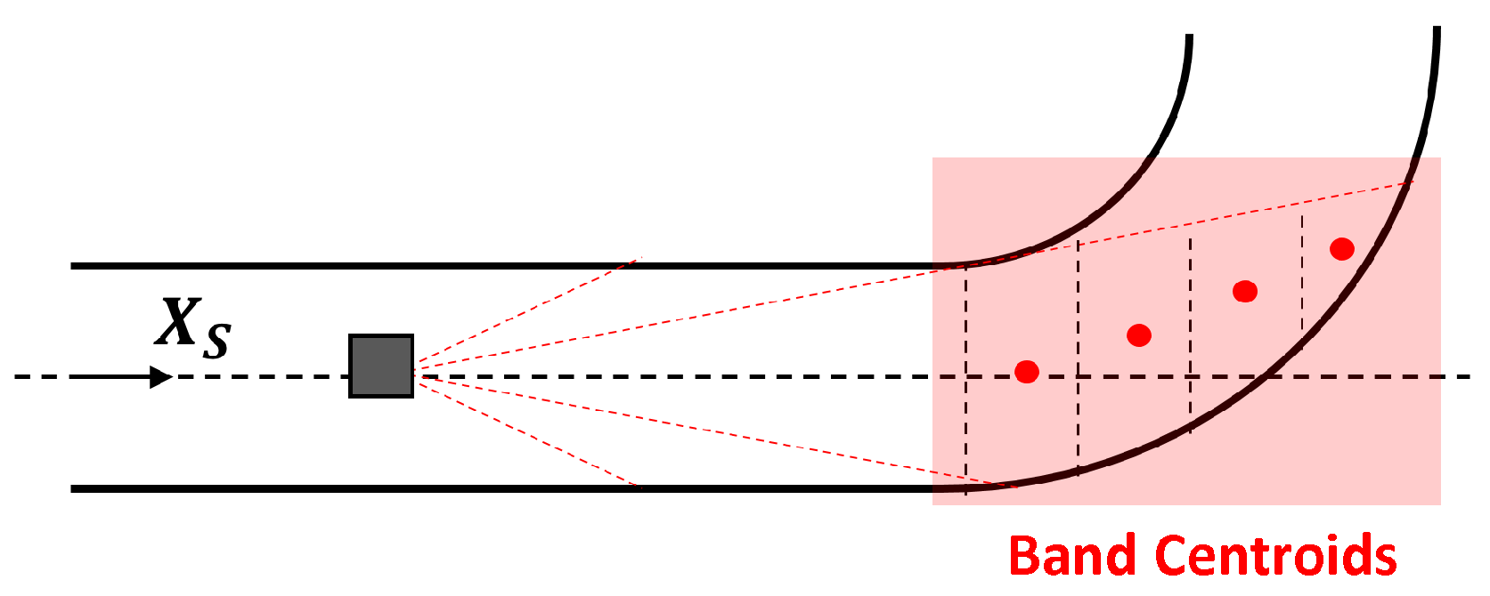
4.3.1. Elbow Direction Estimation Based on Band Centroid

The estimation of elbow direction relies on the observation that the point cloud inside the elbow deviates toward the elbow’s direction compared to the straight pipe. To evaluate this deviation reliably, we propose using X-band and its centroid. Specifically, we classify the point cloud near the elbow area into the X-band along the $X_S$ at intervals of $\delta x_E$, as illustrated in Figure 8. We observe the key geometric property of the point cloud that X-band farther from the camera has more deviation toward the elbow direction. To quantify this deviation, points within each X-band are aggregated into a centroid. The centroid provides a robust estimate by neutralizing random errors from individual points. As the centroid is farther away from the origin, it is more reliable for direction estimation. Therefore, we compute the elbow direction using the weighted average of the direction computed by each centroid. Given N centroids in SCS $(x_{i,S}, y_{i,S}, z_{i,S})(1\le i\le N)$, the elbow direction ${\theta }_E$ is computed as follows:

$${\theta }_E={\displaystyle \frac{{\sum }_{i=1}^N\sqrt{y_{i,S}^2+z_{i,S}^2}arctan\left(\frac{y_{i,S}}{z_{i,S}}\right)}{{\sum }_{i=1}^N\sqrt{y_{i,S}^2+z_{i,S}^2}}}$$

(1)

Given ${\theta }_E$, the elbow plane can be computed. This plane contains $X_S$ and creates angle ${\theta }_E$ with the $X_S{Y}_S$-plane. The elbow plane is an important input for the elbow radius estimation in the following section.

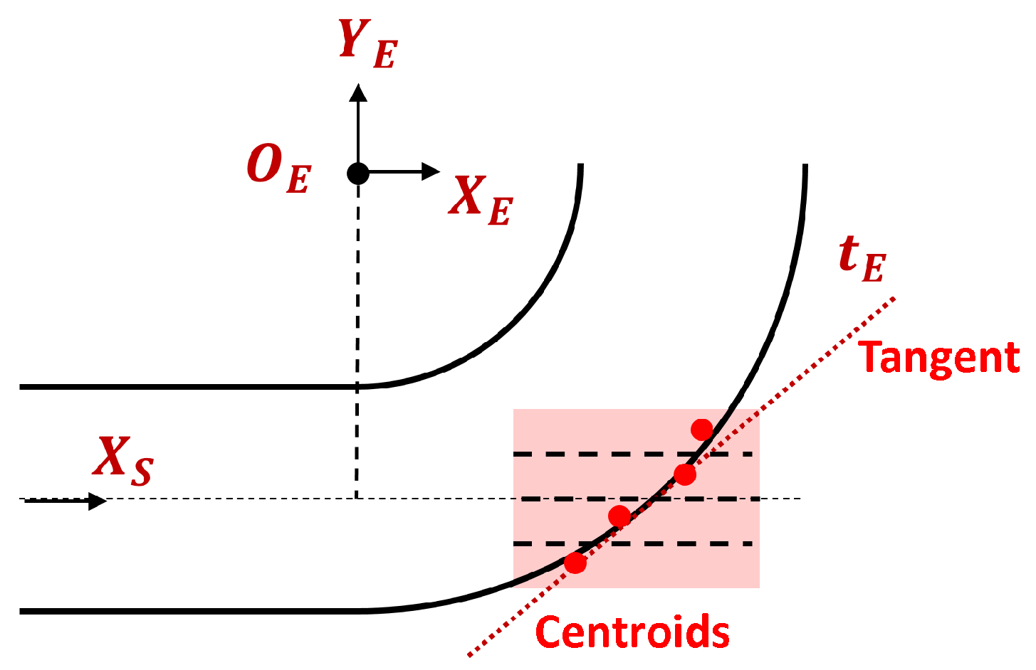
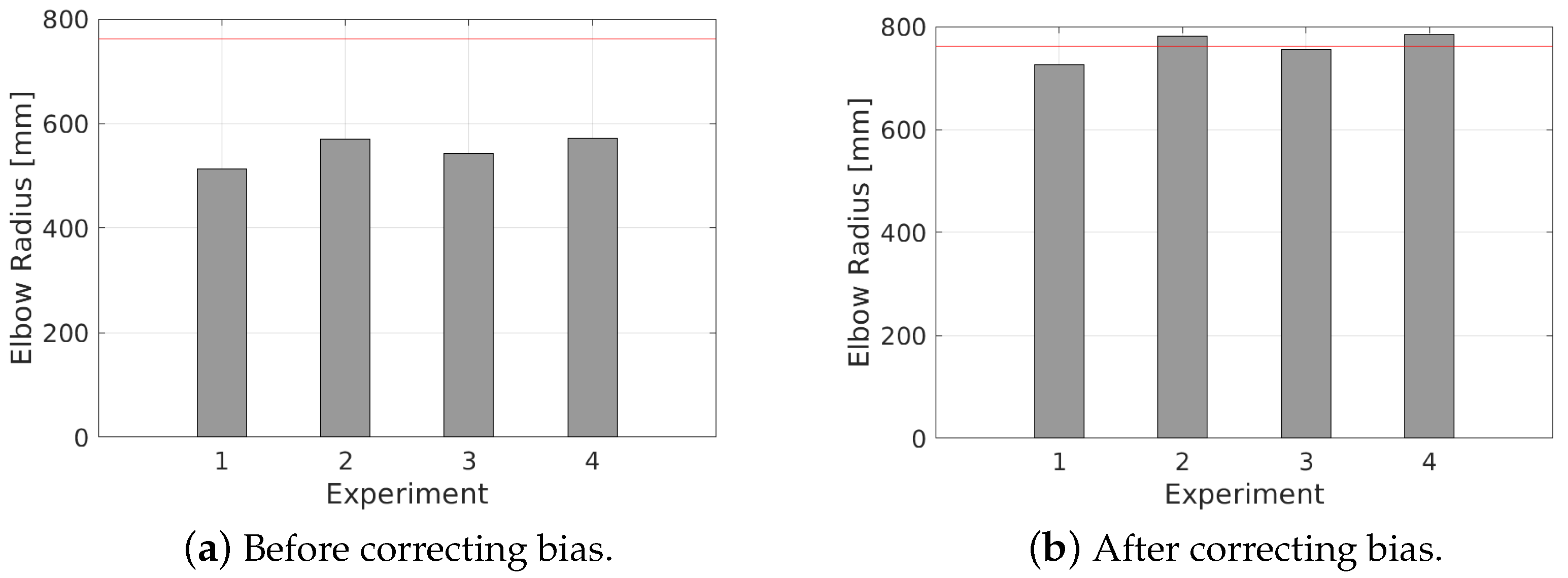
4.3.2. Elbow Radius Estimation Using Tangent Angle

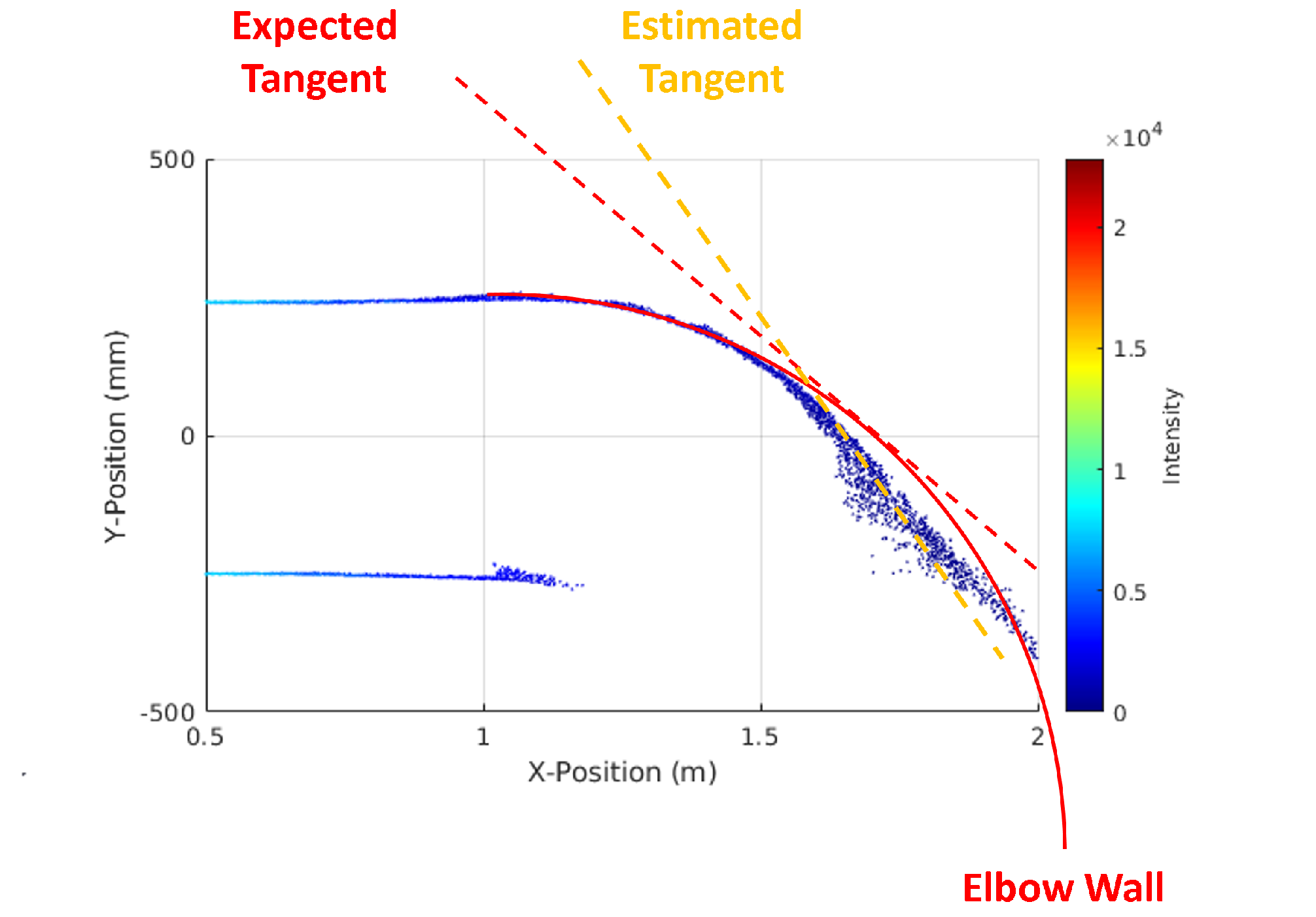
The common approach to finding the elbow radius is typically based on the torus or circle fitting, but it is computationally intensive and often inaccurate due to the incomplete coverage of the torus model. To address this limitation, we propose a simple geometric approach based on the tangent of the elbow in the elbow plane, as shown in Figure 9. Let $T_E$ be the intersection between $X_S$ and the larger inner wall of the elbow on the elbow plane, i.e., $X_E{Y}_E$-plane. The tangent $t_E$ of the elbow at $T_E$ on the elbow plane creates an angle $\gamma$ with $X_S$. $\gamma$ is also equal to angle $\widehat{S_E{O}_E{T}_E}$, and $cos\gamma$ can be computed as follows:

$$cos\gamma ={\displaystyle \frac{R_E}{R_E+r_E}}$$

(2)

From this equation, the elbow radius $R_E$ can be computed as follows:

$$R_E={\displaystyle \frac{r_{E}cos\gamma }{1-cos\gamma }}$$

(3)

To estimate the tangent, we reuse the processing using the band and centroid. We first extract the points from inner outlier points within the $\delta d_E$ distance to the elbow plane. Then, the selected points are classified into Y-bands along the $Y_E$-axis of the elbow, as illustrated in Figure 10. The centroid of each band is calculated to provide a robust representation of the points within the band. Using these centroids, the tangent is estimated, enabling the computation of the tangent angle $\gamma$ and the elbow radius $R_E$.

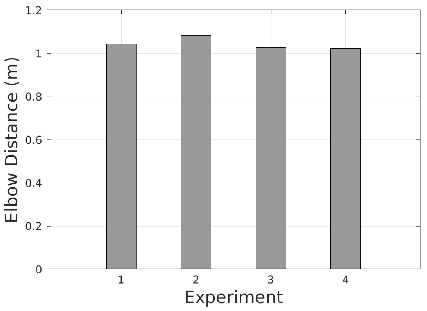
4.3.3. Elbow Distance Estimation

The elbow distance is directly derived from the tangent estimation. As shown in Figure 9, the tangent estimation identifies the location of the tangent point $T_E$. Moreover, the distance from the elbow starting point $S_E$ to tangent point $T_E$ can be computed regarding $R_E$ and $\gamma$ as follows:

$$\overline{S_E{T}_E}=R_{E}tan\gamma$$

(4)

Given the point $T_E$ and the computed distance $\overline{S_E{T}_E}$, we can derive the location of $S_E$ and the distance $\Delta x_E$. From this distance $\Delta x_E$ together with the elbow direction ${\theta }_E$ and elbow radius $R_E$, the origin $O_E$ is the point on the elbow plane and is $R_E$ distance away from $S_E$ along the $Y_E$-axis.

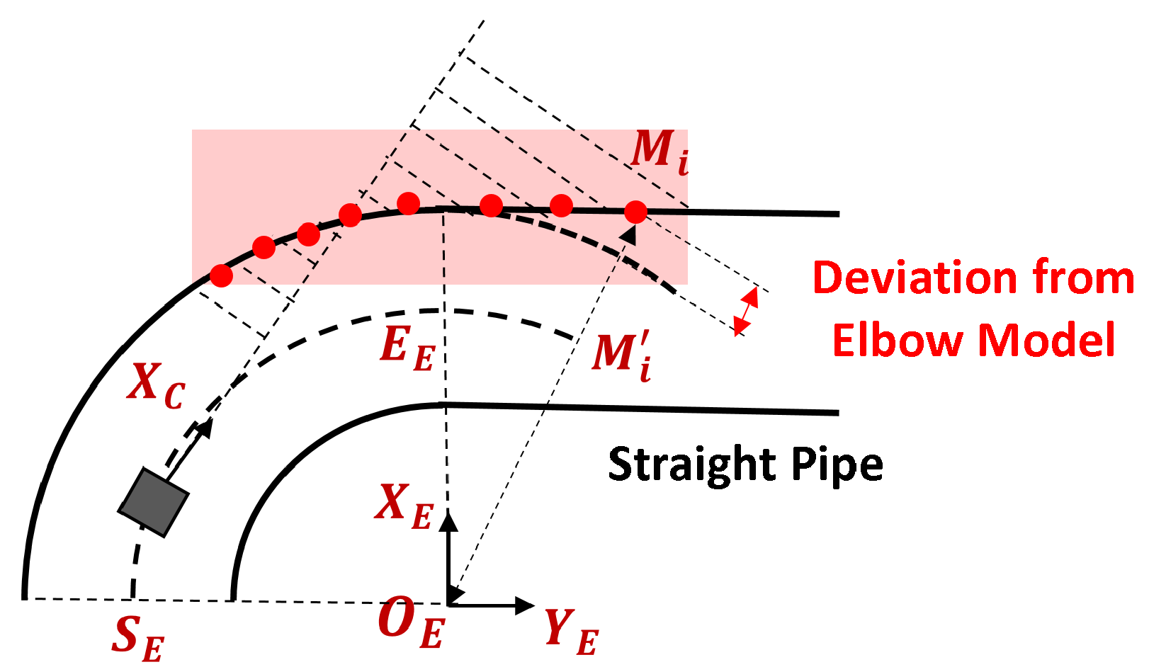
4.3.4. Elbow Length

Determining the elbow length requires identifying the start of the subsequent straight pipe. As the PIG approaches the subsequent straight pipe, portions of the point cloud begin to deviate from the torus shape characteristic of the elbow. To detect this deviation, we first extract points near the elbow plane within a distance of $\delta d_E$ as in elbow radius estimation. The points are then divided into X-band along $X_C$-axis and find the centroid for each band, as shown in Figure 11. If a centroid $M_i$ satisfies the following condition, it is considered to deviate from the elbow torus model:

$$|O_E{M}_i|-R_E\ge \Delta R_E$$

(5)

The centroid $M_i$ satisfying this condition indicates the presence of the subsequent straight pipe. $M_i$ is then projected on the central arc of the elbow to obtain $M_i^{\prime }$, as shown in Figure 11. The elbow length $l_E$ is obtained by compensating $\Delta R_E$ from the length of arc $\stackrel{⌢}{S_E{M}_i^{\prime }}$ to remove the effect of the threshold $\Delta R_E$ as follows:

$$l_E=|\stackrel{⌢}{S_E{M}_i^{\prime }}|-R_{E}arccos{\displaystyle \frac{R_E+r_E}{R_E+r_E+\Delta R_E}}$$

(6)

4.4. T-Junction Estimation

Given that the T-junction is detected, we need to estimate the branch direction, branch radius, distance from the 3D ToF camera, and T-junction length. Similar to the elbow, the branch direction indicates which angle the PIG needs to consider the branch, while the branch radius affects how to control the PIG. The distance and length indicate where the control should be initiated and terminated.

4.4.1. Branch Direction Estimation Based on Band Intensity

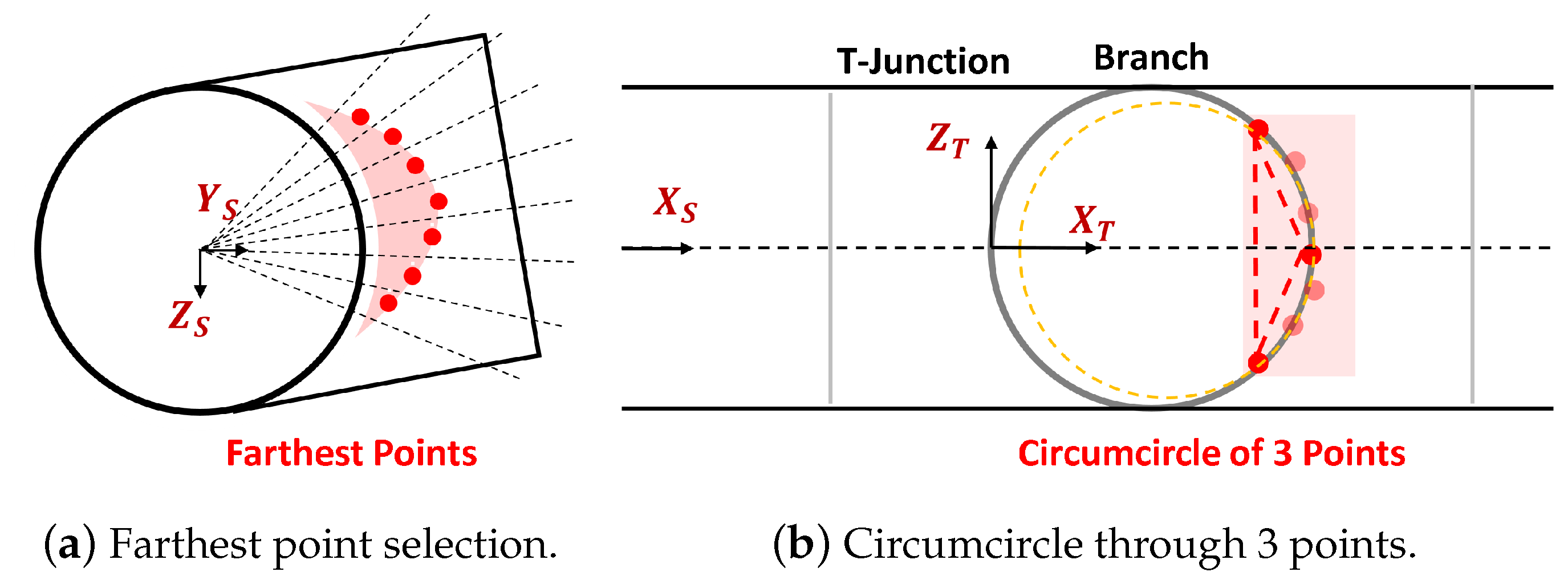
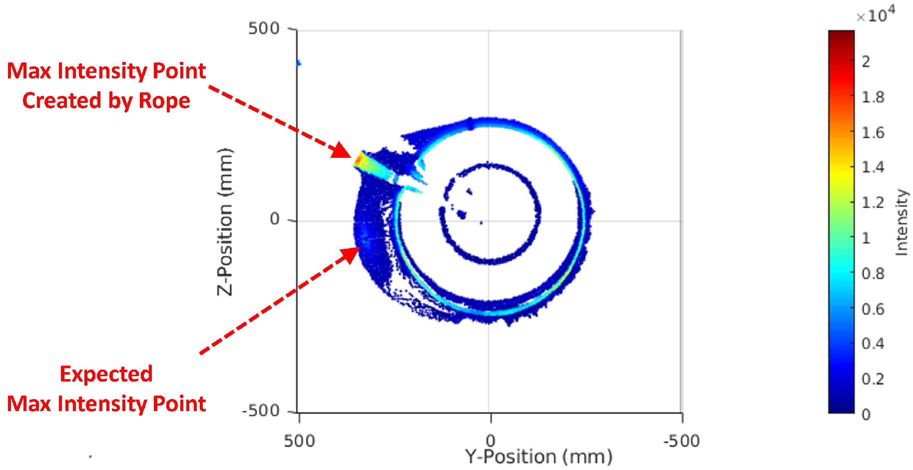
To detect the branch direction, we rely on the fact that an area of points on the branch having high intensities because of small incident angles indicates the branch direction. The highest intensity point indicates the direction of the branch. However, relying solely on the single highest-intensity point for branch direction estimation can be unreliable due to potential intensity errors or the presence of the defect with high intensity. To improve reliability, we propose dividing the outer outlier point cloud into C-band along the circumferential axis in the $Y_S{Z}_S$-plane with an angular step $\delta {\alpha }_T$, as illustrated in Figure 12b. For each band, we compute the average intensity as a feature to reduce the impact of intensity errors and random defects. We select the C-band with the highest average intensity, and inside it we select the highest intensity point. The direction of this point is also the branch direction ${\theta }_T$. Given ${\theta }_T$, the direction of $Y_T$ and $Z_T$ are obtainable. Therefore, the $X_T{Z}_T$-plane is well defined even though the origin $O_T$ is unknown. This plane is used to estimate the branch radius in the following section.

4.4.2. T-Junction Branch Radius Estimation Based on Circumcircle Estimation

We propose a simple geometric solution for branch radius estimation based on estimating the circumcircle through 3 points. It reuses the C-band used for branch direction estimation as illustrated in Figure 13a. We select the farthest points on $Y_S{Z}_S$-plane of each C-band as the feature since these points are located inside the branch. These points are projected to the $X_T{Z}_T$-plane and show the circle shape of the branch, as shown in Figure 13b. To estimate the circle, we select three points from three C-bands. The first point is in the C-band having the highest average intensity. The remaining two points are in the C-bands farthest away from the first C-band. This selection ensures maximum separation of points and improves estimation accuracy. The branch radius is the radius of the circumcircle of the triangle created by the selected three points. Let $d_a$, $d_b$, and $d_c$ be the edge length of the triangle. The radius of circumcircle according to [18,19] is as follows:

$$r_B={\displaystyle \frac{d_a{d}_b{d}_c}{4\sqrt{s(s-d_a)(s-d_b)(s-d_c)}}}$$

(7)

where s is the semiperimeter of the triangle and is computed as $s=(d_a+d_b+d_c)/2$.

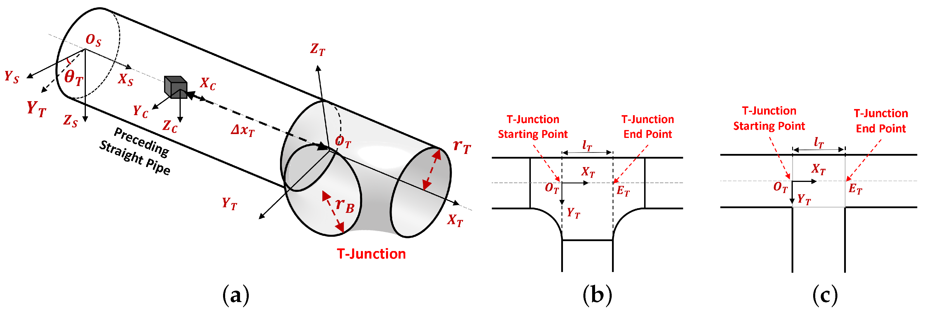
4.4.3. T-Junction Distance and Length Estimation

The T-junction distance is estimated directly based on the branch radius and points used for estimating it. As we can observe from Figure 13, among three points used for branch radius estimation, the point in C-band with the highest intensity can be projected to the $X_T$-axis to get the end point $E_T$. The start point $O_T$ is $2r_B$ distance before the $E_T$ on the $X_S$-axis. By knowing $O_T$, the distance $\Delta x_T$ to the T-junction can be obtained as defined in Figure 3. On the other hand, the T-junction length $l_T$ is obtained directly as the branch diameter $l_T=2r_B$.

5. Real-Time Adaptation

Even though the RT-ETDE framework is designed to be lightweight, further techniques need to be applied to meet the real-time constraint. We apply three techniques including point skipping, language-dependent optimization, and multi-processor offloading. Since the number of points in the point cloud can be extremely large, using all of them incurs a high processing load on the system. Therefore, we apply uniform point skipping where only one out of every $N_P$ points is selected for processing. Via preliminary experiments, we found that $N_p=8$ achieves the balance between detection accuracy and processing time. On the other hand, language-dependent optimization techniques include minimizing the variable allocation, maximizing the use of low-level codes, and using high-speed registers for frequently used variables.

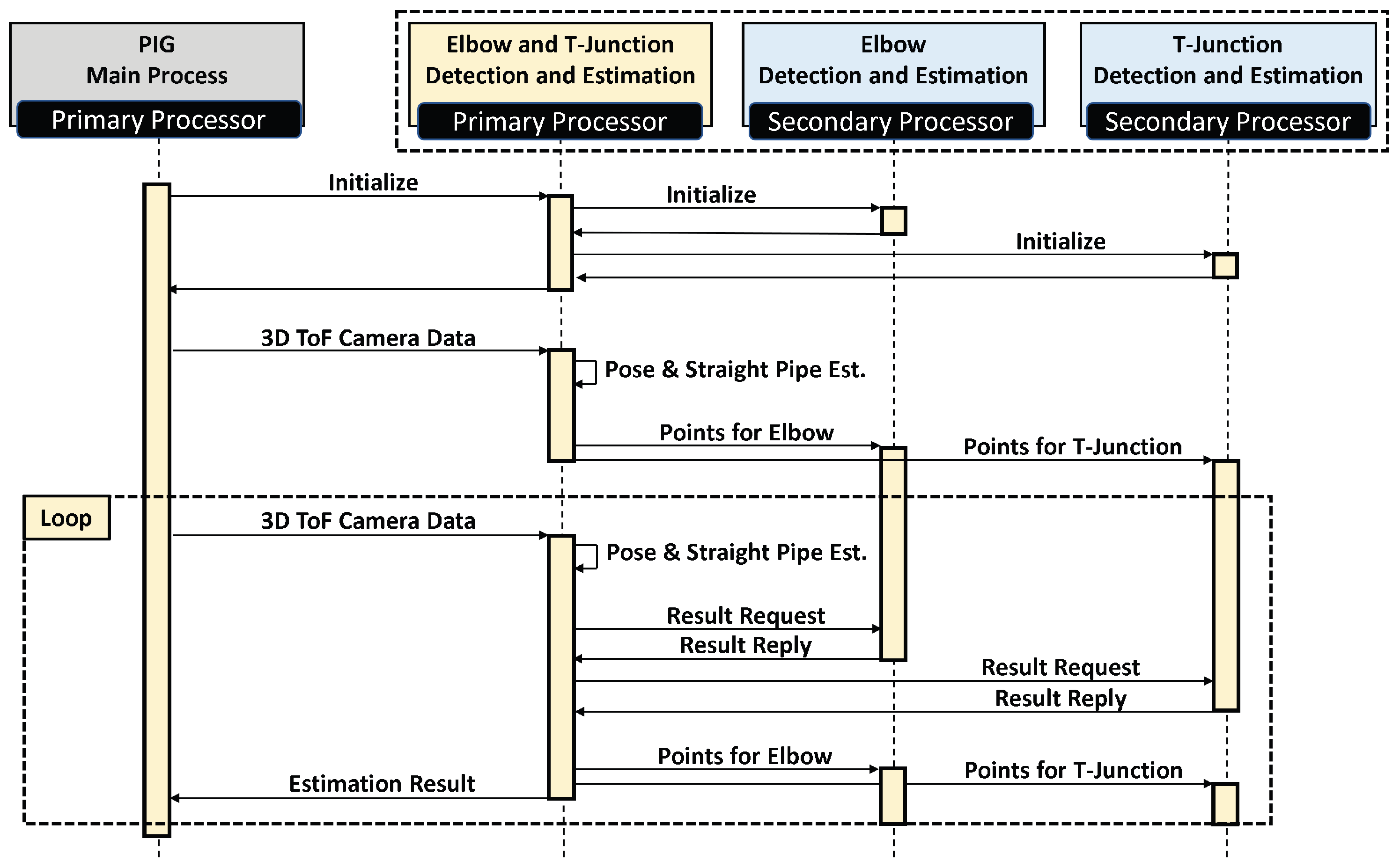
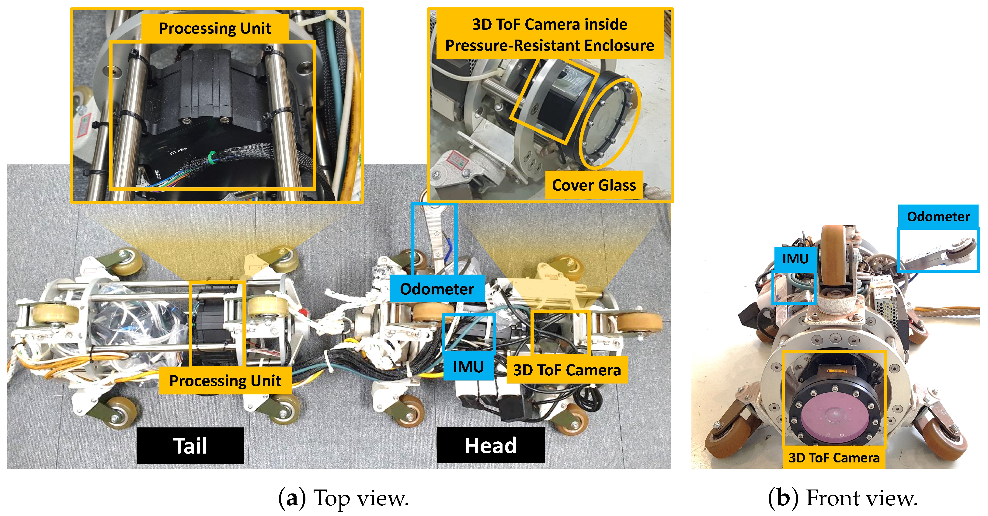
We also propose an offloading scheme for multi-processor systems. Particularly, we apply this scheme to the Xilinx Zynq 7000 processing unit which is used in the real PIG. This system consists of a dual-core ARM Cortex-A9 processor operating at 800 MHz as a primary processor and two Microblaze processors operating at 125 MHz as secondary processors. The primary processor needs to perform all tasks consisting of data collection, processing, and control. The RT-ETDE framework may interfere with these tasks. Therefore, we need to partially offload the RT-ETDE framework to the secondary processors considering their limited processing power.

The detection and detection operation for each feature are extracted to become the elbow detection and estimation (EDE) process and T-junction detection and estimation (TDE) process, respectively. The pose and straight pipe estimation and framework coordination are given to the ETDE process. The ETDE process is located on the master processor for interacting with the PIG main process while EDE and TDE processes are transferred to two secondary processors. Figure 14 shows the sequence diagram of the multi-processor offloading scheme. First, the PIG main processing process initializes the ETDE, EDE, and TDE processes. When the data is available from the 3D ToF camera, it is sent to the ETDE process for processing. The pose and straight pipe are first estimated. Then, points for the elbow and T-junction are extracted and sent to EDE and TDE processes, respectively. The ETDE process does not wait for the result but becomes ready directly for the new data. When the second data comes from the 3D ToF camera, the ETDE process also performs pose and straight pipe estimation as in the first data. However, after that, it directly requests the detection and estimation results of the first data from EDE and TDE processes. Finally, it extracts and sends the points to EDE and TDE processes for detection and estimation. The process of the second data is repeated for the following data. Through this mechanism, ETDE, EDE, and TDE processes run in parallel, therefore saving processing time.

6. Results

In this section, we first describe the experiment setup. Next, the elbow and T-junction detection result is presented, followed by the detailed estimation results for each of the parameters. Finally, we evaluate the processing time of the framework on the real PIG processing unit.

6.1. Experiment Setups

To evaluate our proposed approach, we develop a pull-rig robot and a 20-inch prototype pipeline. Figure 15 shows the prototype pipeline consisting of four 6-m straight pipes, one 1.5D elbow, and one T-junction with the same shape and size as the real gas pipeline. The 1.5D elbow has a radius of 1.5 times the pipe diameter, which is 762 mm. The elbow angle is 90°, which has a length of 1.196 m. The T-junction branch has the same radius as the main pipe.

Figure 16 shows the robot and its components. The robot consists of two parts: a head and a tail, each of which is equipped with passive wheels to move along the pipeline. A rope is attached to the front and the end of the robot to pull the robot forward and backward. The main components of the robot include a Helios2 3D ToF camera, an IMU, an odometer, and a processing unit which are distributed on the tail and head parts, as in Figure 16. The robot speed is approximately 0.5 m/s when approaching the elbow and T-junction. The processing unit is the Xilinx Zynq 7000 system, which is the same as the one used in the real PIG.

To address the high-pressure environment in gas pipelines, the 3D ToF camera needs a pressure-resistant enclosure with a cover glass that is strong enough for the pressure and has minimal effect on the measurement. Types of glass are considered for the cover glass, including tempered glass, polycarbonate, and polymethyl methacrylate. The selection criteria for the cover glass are twofold: (1) the flexural strength, i.e., the strength against the bending, and (2) the transmittance, i.e., the ratio of light that can go through the glass.

Table 2. Comparison of cover glass types.

Type of Glass	Flexural Strength (MPa)	Transmittance (%)
Tempered glass	120	66.0
Polycarbonate	96	88.9
Polymethyl methacrylate	108	92.1

shows these criteria on 10-mm thickness glasses of each type. We choose polymethyl methacrylate as the cover glass material which has the best transmittance and the second highest flexural. We verify with the pressure test that the enclosure with polymethyl methacrylate cover glass can endure the real pipe pressure. On the other hand, we address another key issue of the cover glass, which is the interference from the internal reflection, as shown in Figure 17. When the light travels from the glass to the outer environment, part of it is reflected back into the glass (red arrow). Through multiple reflections, it may reach the receiver and interfere with the actual returning light from the object (orange arrow). To alleviate this issue, the anti-reflection coating is applied to the glass.

Table 3. Transmittance improvement of polymethyl methacrylate after anti-reflection coating.

Type of Coating	Transmittance (%)
Without coating	92.1
One-side coating	93.9
Both-side coating	96.9

shows the transmittance before and after coating on one or both sides. We select both-side coating since it has the highest transmittance, i.e., the lowest interference.

The Helios2 3D ToF camera has a resolution of 640 × 480 and a field of view of 69° × 51°. The frame rate is fixed at 10 Hz. Figure 18 shows three point clouds without and with the existence of the elbow and T-junction. Data points with an X-position below 0.5 m do not completely cover the circumferential direction of the pipe while data points with an X-position above 2.0 m do not show the correct pipe shape or are randomly invalid, as illustrated in Figure 18a. Therefore, we choose the data points with an X-position between 0.5 and 2 for processing. Moreover, the data points within (1.2, 2) m are used for ETDE, while the range (0.5, 1.2) is used for camera pose estimation. Figure 18b,c show the point cloud of the elbow and T-junction in this range.

We perform four experiments with different robot roll angles at the entry point, i.e., (0°, 90°, 180°, 270°). Figure 19 shows the camera coordinate system and the first straight pipe coordinate system, as well as the rear view of the robot at the entry point of the pipeline. Note that the robot Z-axis has the same direction as the 3D ToF camera Z-axis. In each experiment, the robot enters the pipeline via the entry point at the given roll angle and moves inside of the pipeline, along the yellow arrow from the straight pipe to the 1.5D elbow, then the straight pipe, and a T-junction to detect and estimate the elbow and T-junction parameters, as described in Section 3.2. The results from four experiments are used to verify the consistency of the detection and estimation. The parameters used in RT-ETDE are summarized in

Table 4. RT-ETDE framework parameters.

Parameter	Value	Unit
$r_E$: Pipe radius of the elbow	242.1	mm
M: Number of points for pose and straight pipe estimation	64	-
${\delta }_B$: Band size for pose and straight pipe estimation	50	mm
$\delta r$: Annulus size for elbow and T-junction detection	20	mm
$\delta x_E$: X-axis band size for elbow direction estimation	100	mm
$\delta d_E$: Distance to $X_E{Y}_E$-plane for elbow radius estimation	50	mm
$\delta {\alpha }_T$: Circumferential band size for T-junction direction estimation	5	$°$

.

6.2. Elbow and T-Junction Detection

Figure 20 shows the pipe types detected by the RT-ETDE framework regarding the navigation distance from the entry point. The result shows that the elbow and the T-junction are successfully detected in all four experiments. There is a difference of up to 0.2 m in the elbow start position and 0.4 m in the T-junction start position. It does not solely come from the detection scheme but is contributed by the slight difference in the start position at the entry point. Moreover, the start position of the T-junction is also affected by the odometer value when traveling through the elbow due to the difference in the starting roll angle at the entry point.

6.3. Elbow Estimation

6.3.1. Elbow Direction Estimation

Figure 21 shows the elbow direction estimation of four experiments. There are no significant differences in the estimation results among the four experiments. The maximum difference is 3.72° between experiments 2 and 3. The mean elbow direction is 7.31°, and the standard deviation is 1.66°. The maximum difference and the standard deviation are considered to be small enough for the PIG control.

Although it is not possible to collect the exact ground truth of the elbow direction, according to Figure 15 the direction of the elbow is to the right, i.e., along the positive direction of the straight pipe $Y_S$-axis. We expect the elbow direction is close to 0°. Therefore, the mean value of 7.31° is reasonable and consistent with this observation.

6.3.2. Elbow Radius Estimation

Figure 22a shows the estimation result of the elbow radius. The red line shows the designed radius of the elbow, which is 762 mm. We can see from the result that the robot underestimates the elbow radius. The mean estimated radius is 549.27, which is 28% smaller than the designed radius. This issue comes from the distortion of the point cloud in the elbow due to the multipath problem. Figure 23 shows an example of the point cloud near the elbow plane that is used for tangent estimation. Around the area for tangent estimation, the point cloud tends to be distorted toward the inner direction and has a much higher random error compared to other areas. As a result, the estimated tangent is much steeper than the expected tangent from the elbow model. It leads to smaller elbow radius estimation.

On the other hand, according to the result in Figure 22a, the standard deviation is 27.06 mm and is about 3.5% of the radius, which is a small value. It indicates that the distortion in Figure 23 is relatively consistent. Therefore, the bias in elbow radius estimation can be corrected experimentally. Figure 22b shows the elbow radius estimation result after bias correction with the design radius. However, the results of elbows with different radii need to be collected and tested to get the common bias correction value.

6.3.3. Elbow Distance Estimation

Figure 24 shows the result of the elbow distance estimation at the first detection. Here, the ground truth of the distance cannot be measured since the robot is inside of the pipeline; therefore, we focus on the farthest distance that the robot can estimate the elbow rather than the accuracy of distance estimation. The result shows that the RT-ETDE framework can detect the elbow at least 1.02 m away from the start of the elbow and on average 1.04 m with a standard deviation of 0.03 m. Detecting the elbow at a distance greater than 1.0 m is crucial, as it ensures sufficient time for PIG systems to activate the control mechanism. Given that PIGs typically operate at an average speed of 2.5 m/s, reaching up to 6.0 m/s [20], a 10-Hz control system allows approximately 1.7 control cycles to process the detection and trigger the control mechanism before the robot enters the elbow.

6.3.4. Elbow Length Estimation

Figure 25 shows the result of the elbow length estimation. The ground-truth elbow length is represented by the red line. Except for experiment 1, all the other experiments slightly underestimated the elbow length. However, the error is less than 0.085 m, which is approximately 7% of the elbow length. It is also relatively small compared to the size of PIG and, therefore, acceptable for PIG control.

6.4. T-Junction Estimation

6.4.1. T-Junction Branch Direction Estimation

Figure 26 shows the result of T-junction branch direction estimation. We can observe that the estimation in experiment 3 has more than a 21° difference compared to the other experiments. This issue comes from the blocking of the rope in front of the 3D ToF camera and creates an area of outlier points with very high intensity as can be seen in Figure 27. Fortunately, this rope only exists in this pull-rig robot and not in the real PIG. Therefore, the direction estimation in experiment 3 can be excluded.

Except for experiment 3, the branch direction estimation variates from −6.89° in experiment 1 to −0.13° in experiment 4. The average branch direction is −4.07°, and the standard deviation is 3.51°. Similar to the elbow, the ground truth of the T-junction branch direction cannot be measured, but it points to the right of the preceding straight pipe, as shown in Figure 15. Therefore, the mean value of −4.07° is also consistent with this observation. On the other hand, the standard deviation of the T-junction branch direction is two times bigger than in the elbow direction because the area of the point cloud used in this case is much smaller than the elbow direction estimation.

6.4.2. T-Junction Branch Radius Estimation

Figure 28 shows the estimation result of the T-junction branch radius. The horizontal red line shows the designed radius of the branch of 246.10 mm. Two experiments are overestimating and two others underestimating the radius. The mean estimated radius is 239.32 mm, while the standard deviation is 17.25 mm. The bias of the estimation is less than 7 mm, which is less than 3% of the radius. The standard deviation is about 7% of the radius. The bias and the standard deviation are acceptable for the PIG navigation. Since T-junction length is equal to branch diameter, this result also reflects the T-junction length estimation.

6.4.3. T-Junction Distance Estimation

Figure 29 shows the estimation result of T-junction distance at the first detection. As for the elbow, the ground truth of the distance cannot be measured; therefore, we focus on the farthest distance that the robot can estimate the T-junction. The result shows that the RT-ETDE framework can detect the T-junction at least 1.28 m away from the start of the T-junction branch and on average 1.47 m, with a standard deviation of 0.15 m. Similar to the elbow, the T-junction is also detected at a distance greater than 1.0 m, providing sufficient time to activate the control mechanism before the robot reaches the junction.

6.5. Maximum Processing Time

To evaluate the real-time constraint of the RT-ETDE framework, we measure the maximum processing time on each processor.

Table 5. Maximum processing time.

Process	Processor	Maximum Processing Time (ms)
ETDE process	Arm Cortex-A9	13.3
EDE and TDE processes	Microblaze	95.3

shows the measurement results. It shows that ETDE process only takes 13.3 ms on a single core of the dual-core Arm Cortex-A9 processor. Therefore, the load on the processor is just 6.65% at a 10-Hz frame rate. It leaves enough processing capacity for other important processing on the PIG, such as data collection and control. On the other hand, EDE and TDE processes take up to 95.3 ms, which is a nearly full load of the Microblaze at a 10-Hz frame rate. We can see that the multi-processor offloading scheme successfully exploits the Microblaze secondary processors to reduce the processing load of the primary processor while the lightweight RT-ETDE framework and other real-time adaptation techniques allow all processors to meet the real-time 10 Hz requirement.

7. Conclusions

In this paper, we propose the RT-ETDE framework to address the challenges of detection and parameter estimation for elbows and T-junctions in natural gas pipeline inspection. The framework employs intelligent point cloud partition and feature extraction combined with simple geometric solutions to minimize computational complexity. Furthermore, the real-time adaptation techniques are presented to ensure the real-time constraint. Experimental results validate the effectiveness of the proposed RT-ETDE framework. It is shown that the RT-ETDE framework consistently detects elbows and T-junctions at a minimum distance of 1 m with reliable estimation of critical parameters. The direction of the elbow and T-junction standard deviation is less than 4°, and the average estimation error of elbow radius, elbow length, and T-junction branch radius is less than 5%. With a 10 Hz frame rate on the real PIG processing unit, the framework demonstrates suitability for deployment in real pipeline inspection gauges (PIGs). Future work will extend the framework to detect and estimate significant thickness changes and heavy welds to make a complete set of solutions for modern autonomous PIGs. Additionally, testing on full-scale pipelines in operational environments will provide further validation of the framework’s performance and robustness.