Article

A Comparative Analysis of Hyper-Parameter Optimization Methods for Predicting Heart Failure Outcomes

by
Qisthi Alhazmi Hidayaturrohman
1,2 and
Eisuke Hanada
3,*
1
Faculty of Engineering, Universitas Pembangunan Nasional Veteran Jakarta, Jakarta 12450, Indonesia
2
Graduate School of Science and Engineering, Saga University, Saga 840-8502, Japan
3
Faculty of Science and Engineering, Saga University, Saga 840-8502, Japan
*
Author to whom correspondence should be addressed.
Appl. Sci. 2025, 15(6), 3393; https://doi.org/10.3390/app15063393
Submission received: 7 February 2025 / Revised: 13 March 2025 / Accepted: 18 March 2025 / Published: 20 March 2025

Abstract

:
This study presents a comparative analysis of hyper-parameter optimization methods used in developing predictive models for patients at risk of heart failure readmission and mortality. We evaluated three optimization approaches—Grid Search (GS), Random Search (RS), and Bayesian Search (BS)—across three machine learning algorithms—Support Vector Machine (SVM), Random Forest (RF), and eXtreme Gradient Boosting (XGBoost). The models were built using real patient data from the Zigong Fourth People’s Hospital, which included 167 features from 2008 patients. The mean, MICE, kNN, and RF imputation techniques were implemented to handle missing values. Our initial results showed that SVM models outperformed the others, achieving an accuracy of up to 0.6294, sensitivity above 0.61, and an AUC score exceeding 0.66. However, after 10-fold cross-validation, the RF models demonstrated superior robustness, with an average AUC improvement of 0.03815, whereas the SVM models showed potential for overfitting, with a slight decline (−0.0074). The XGBoost models exhibited moderate improvement (+0.01683) post-validation. Bayesian Search had the best computational efficiency, consistently requiring less processing time than the Grid and Random Search methods. This study reveals that while model selection is crucial, an appropriate optimization method and imputation technique significantly impact model performance. These findings provide valuable insights for developing robust predictive models for healthcare applications, particularly for heart failure risk assessment.

1. Introduction

Approximately 64 million people worldwide have heart failure, and it is one of the world’s most deadly diseases, according to the WHO [1]. Due to the uncertainty of disease progression, predicting the outcome of heart failure is challenging. Readmission and mortality risk are two common outcomes that researchers use to predict the risk of heart failure [2]. Researchers use various approaches to building their models, and machine learning has become one of the most popular and effective methods [3].
Landicho et al. compared four machine learning-based models for predicting the readmission of patients with heart failure, along with a cost analysis. Their support vector machine-based model achieved an accuracy of 0.610 and outperformed the other three models [4]. However, the study did not mention imputation techniques for handling missing values. Plati et al. proposed a machine learning approach incorporating feature selection and handling class imbalance to diagnose chronic heart failure (CHF) based on an electronic health records-based dataset, with an accuracy of 91% for the classification of CHF [5]. Utilizing the dataset of a public database, MIMIC-III, Li et al. used an XGBoost algorithm as their classifier when building a predictive model for in-hospital mortality that had good calibration, with an AUC score of 0.8416 compared to an AUC of 0.7747 for their Get With the Guidelines-Heart Failure (GWTG-HF) risk score model [6].
Designing optimal machine learning-based models is challenging due to the variety of datasets and the complexity of the algorithms used for building predictive models [7]. To obtain the optimal model, the hyper-parameter of the model needs to be tuned to fit a specific dataset. Because a clinical-based dataset consists of complex variables, tuning the hyper-parameter manually is extremely expensive and time-consuming [8]. Applying an optimization method to find the ideal hyper-parameter for each algorithm provides an efficient way to tune the model.
Grid Search has become popular for optimizing machine learning and has been used in multiple studies, specifically for the prediction of heart disease and heart failure [9,10,11]. The simplicity of the Grid Search method allows researchers to optimize their models [11]. Asif et al. utilized Grid Search to obtain optimal configurations for their heart disease prediction models, resulting in slight improvement in terms of accuracy [12]. However, due to the brute force characteristic of Grid Search, the optimization process takes more time in some cases. Valarmathi and Sheela conducted a comparative study of the Grid Search and Random Search optimization methods, reporting that Random Search needed less processing time and provided better performance than Grid Search [13]. Moreover, Sharma et al. proved that Random Search optimization was able to adequately tune their hybrid deep neural networks model for predicting coronary heart disease [14]. Gao and Liu et al. promoted the use of Bayesian hyper-parameter optimization to optimize ensemble learning-based models in the field of medical informatics, including cardiovascular disease prediction [15,16]. They reported that the Bayesian optimization method provided better stability when finding the optimal hyper-parameter than the Grid and Random Search methods. However, their study did not carry out a performance comparison of the three optimization methods.
In this study, we used a comparative analysis approach with two methods commonly used for Bayesian-based optimization to build predictive models for heart failure risk prediction based on a real-patient dataset. While the Grid Search and Randomized Search methods are more common and easier to apply, we found that Bayesian Search has the potential to provide better performance. This study is a classification metrics-based evaluation performed to compare the above three optimization methods. The study was carried out as follows:
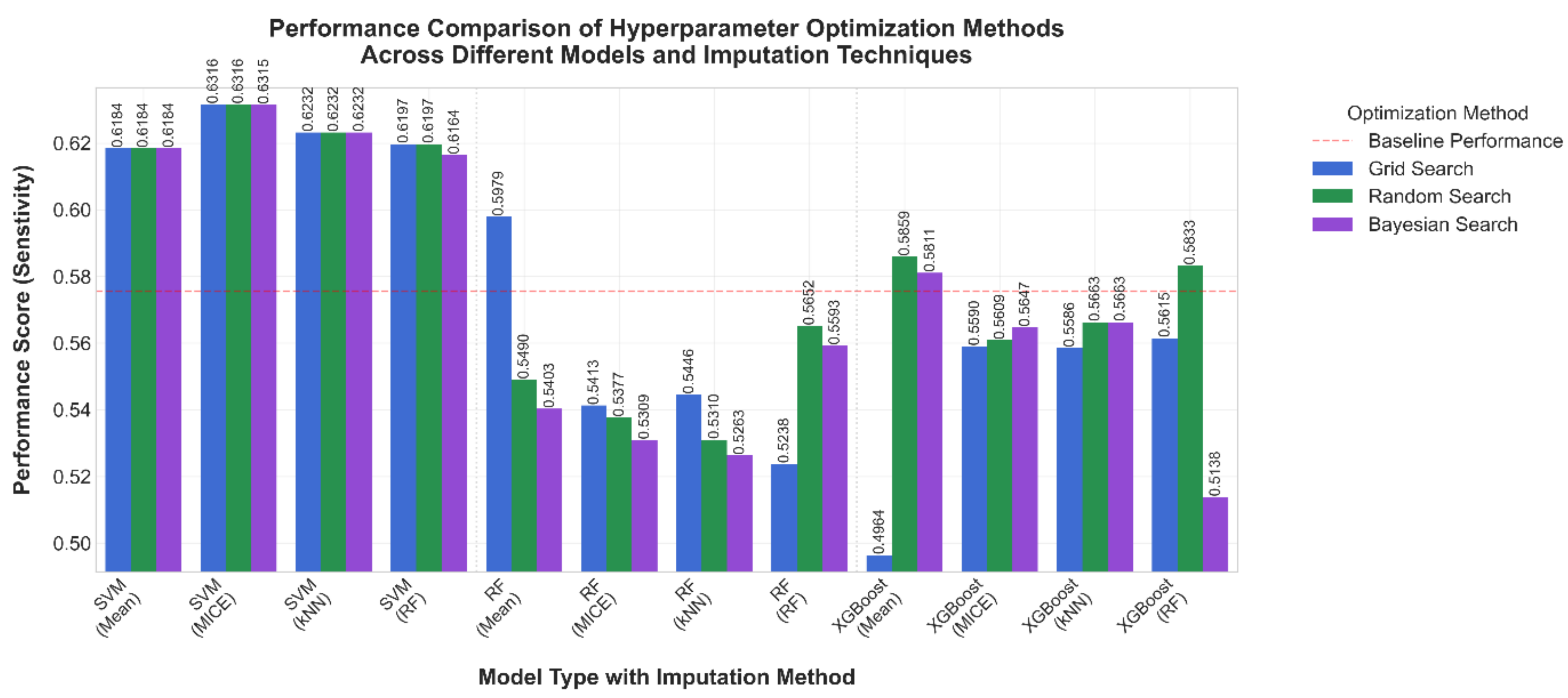
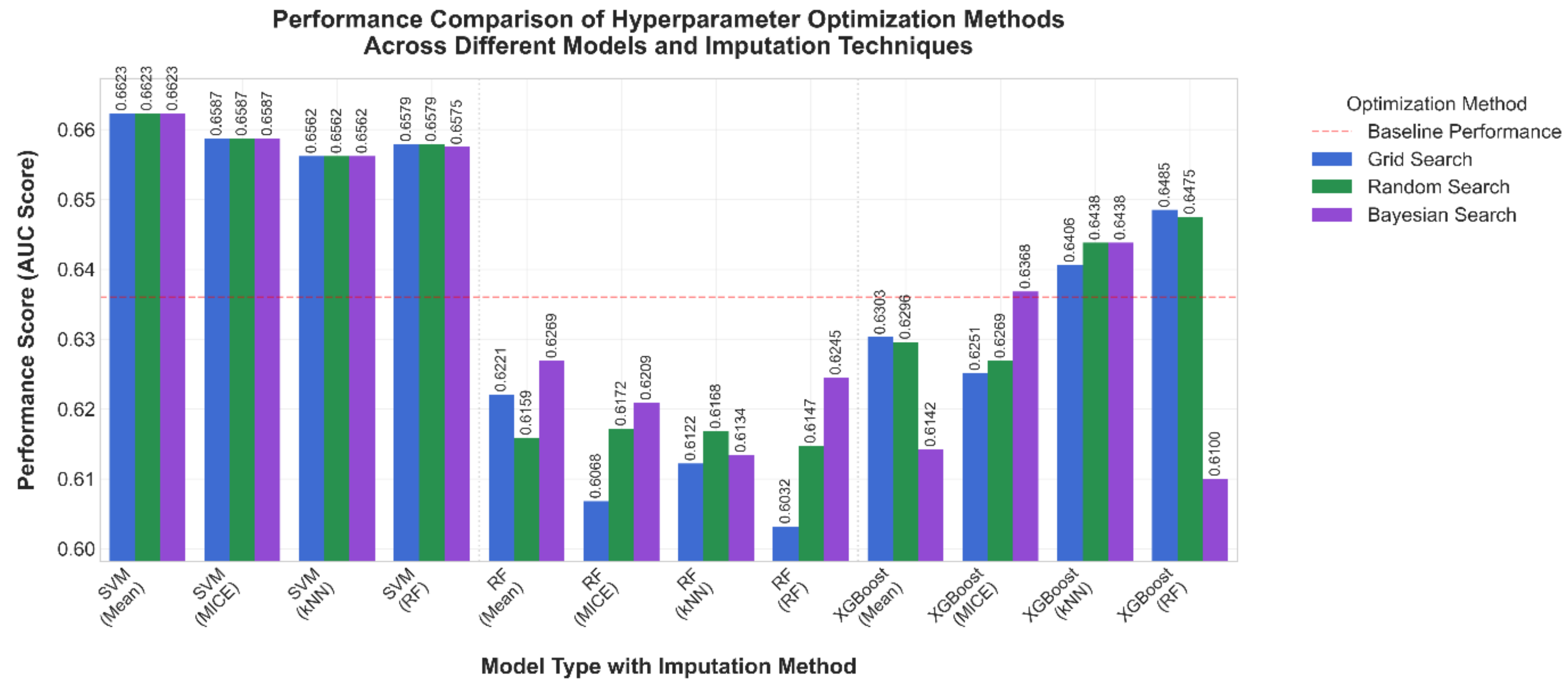
  • The Support Vector Machine, Random Forest, and eXtreme Gradient Boosting algorithms were used to evaluate and compare the effectiveness of the Grid, Random, and Bayesian search methods in determining the ideal configuration for optimizing the performance of a model.
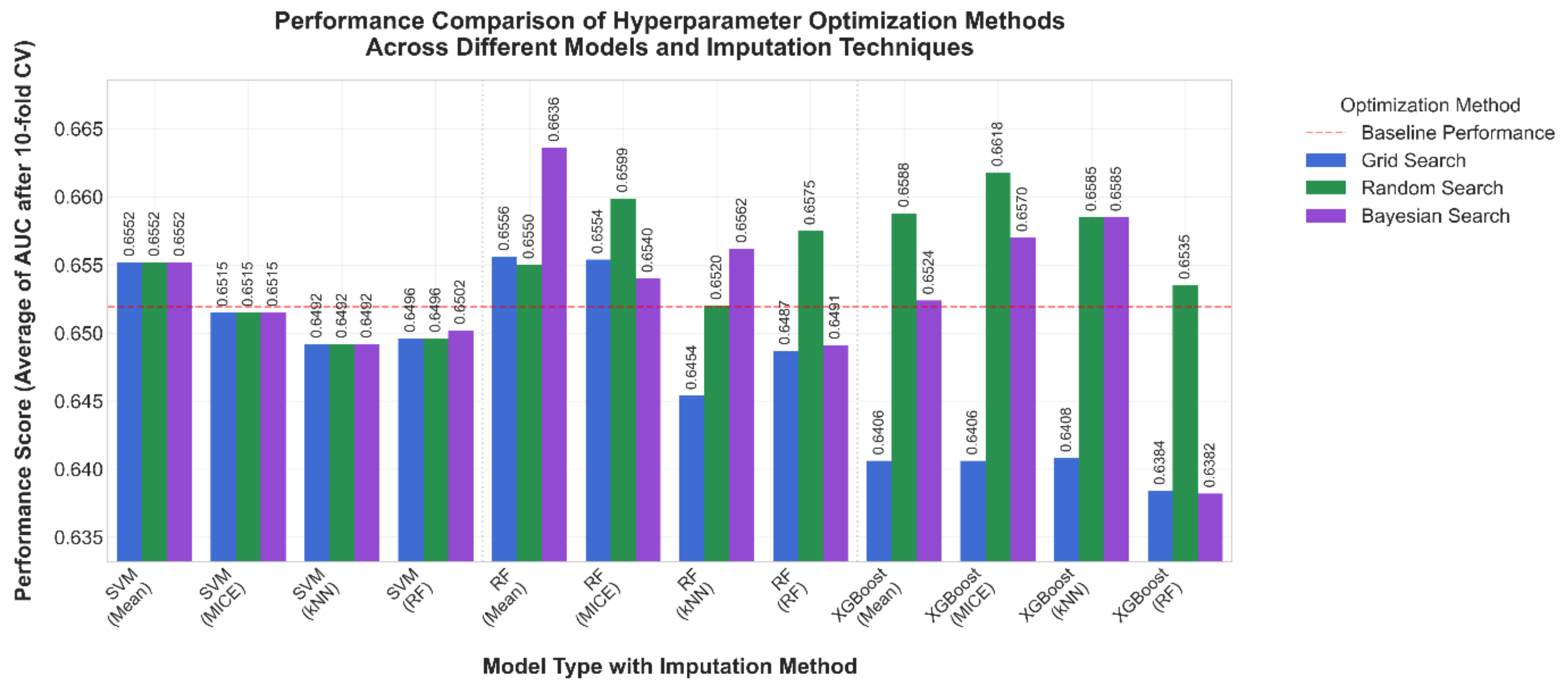
  • The robustness of the proposed models was examined through comprehensive 10-fold cross-validation.
While several recent studies have applied machine learning techniques to predict heart failure outcomes, most have focused either on single-model performance or on limited aspects of hyper-parameter tuning [3,4,5,6,9,10,12]. In contrast, our study provides a unique, comprehensive comparison of three hyper-parameter optimization methods—Grid Search, Randomized Search, and Bayesian Search—across three distinct algorithms (SVM, RF, and XGBoost) while also systematically investigating the impact of multiple imputation techniques on model performance. By employing a real-world clinical dataset and validating the models through rigorous 10-fold cross-validation, our study not only demonstrates predictive performance and robustness comparison but also compares the computational processing time of each model. This integrated approach fills an important gap in the literature by offering a methodological framework that can be generalized to other clinical prediction problems.

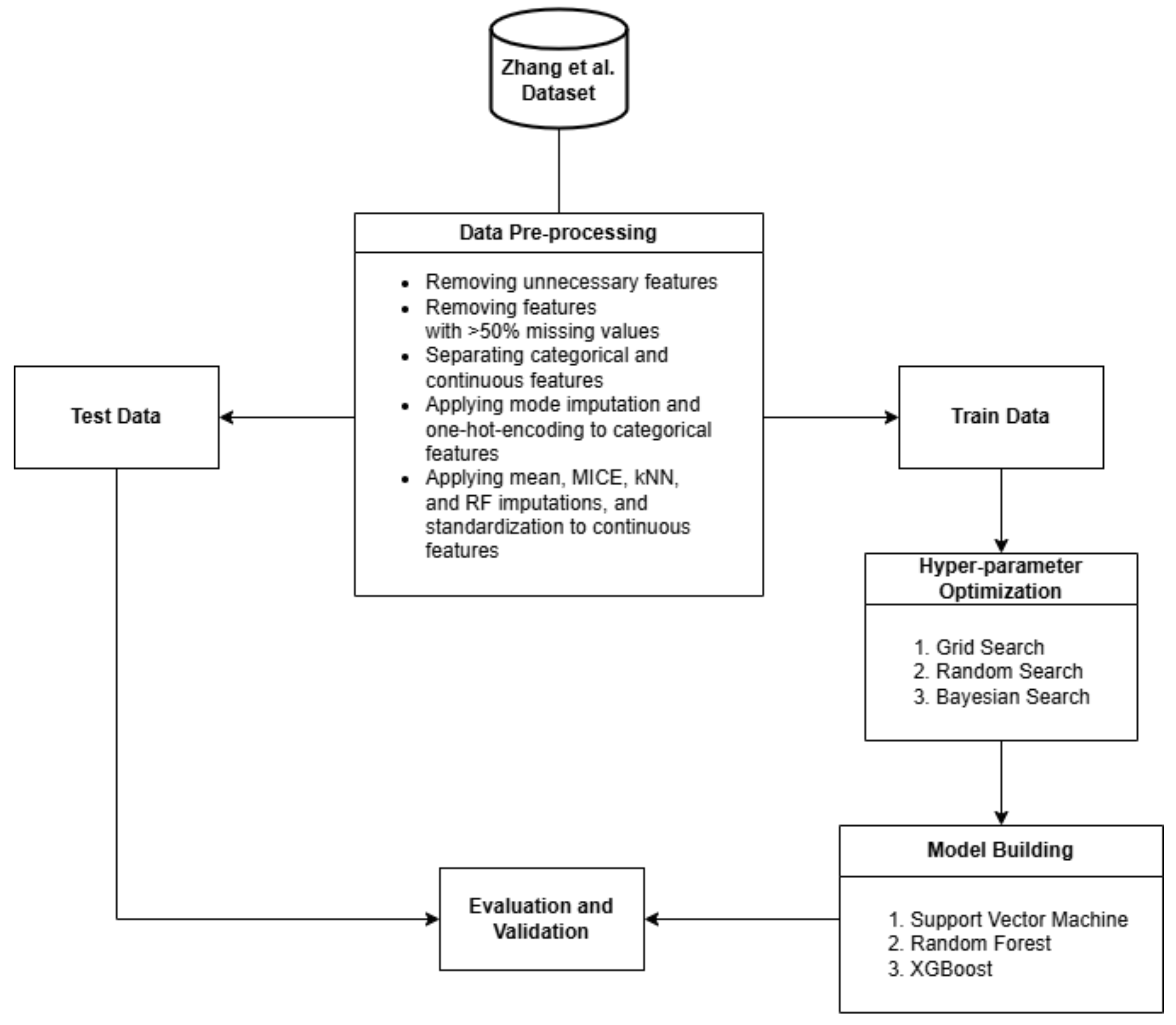
2. Materials and Methods

2.1. Dataset

This study used data from real patients diagnosed with heart failure collected at Zigong Fourth People’s Hospital, China, by Z. Zhang et al. between December 2019 and June 2019 as part of a large cohort study [17]. The diagnosis followed the European Society of Cardiology (ESC) criterion for the diagnosis of heart failure. The dataset consists of 167 features for 2008 patients, both continuous and categorical [17,18]. In addition to baseline clinical characteristics like blood pressure, respiratory rate, temperature, pulse rate, and laboratory findings, the dataset contains data on six possible outcomes, including mortality and readmission, which were separated by different time windows.

2.2. Preprocessing

We used an approach to pre-processing similar to that of our previous study [19]. Of the 167 features in the dataset, we removed eight that were not essential for predictive model building, none of which impacted the outcome of the model. The dataset has six possible outcomes, including readmission and mortality within six months, which we combined to allow greater focus on all-cause readmission and mortality prediction. For comparison purposes, we used the mean, Multivariable Imputation by Chained Equations (MICE), k-Nearest Neighbor (kNN), and Random Forest (RF) imputation techniques for the handling of missing values. We applied these imputations to continuous features that had missing values less than or equal to 50%. Mode imputations were applied to the categorical features [20]. Features with more than 50% missing values were excluded.
One-hot encoding was used to encode the categorical features into an integer type [21]. By applying one-hot encoding, a new variable was created for each categorical output, with the variable containing a binary output of 0 or 1. To standardize the value of each continuous feature, we applied a standardization approach known as z-score normalization [22]. This approach transformed each continuous feature into a standard score with a mean of 0 and variation of 1 through the following formula [23]:
z = x μ σ
We obtained the standardized value of the feature (z) by subtracting the original data point of feature (x) with its mean (μ) to center it and then dividing it by the standard deviation (σ) to scale it.

2.3. Hyper-Parameter Optimization

2.3.1. Grid Search and Randomized Search

Both Grid Search (GS) and Randomized Search (RS) are traditional model-free algorithms-based optimization methods for hyper-parameter optimization [7]. One of the most commonly used optimization approaches, Grid Search (GS), uses a brute-force method to evaluate an entire given hyper-parameter combination and has been shown to have good performance [11]. GS involves defining a set of possible values for each hyper-parameter and exhaustively evaluating all combinations. In addition to the comprehensive process this method provides, implementing GS is simpler than with other optimization methods [24]. While comprehensive, this method can be computationally expensive for large hyper-parameter spaces [25].
Unlike GS, Randomized Search, also called Random Search (RS), performs random selection by evaluating all given hyper-parameters instead of testing them one by one in sequences [26,27]. This method can also be easily applied to optimize machine learning-based models. RS is more efficient than GS but has less of the computational processing resources required for large search spaces [28]. Figure 1 below shows the difference between Grid Search and Random Search in terms of optimizing the models.

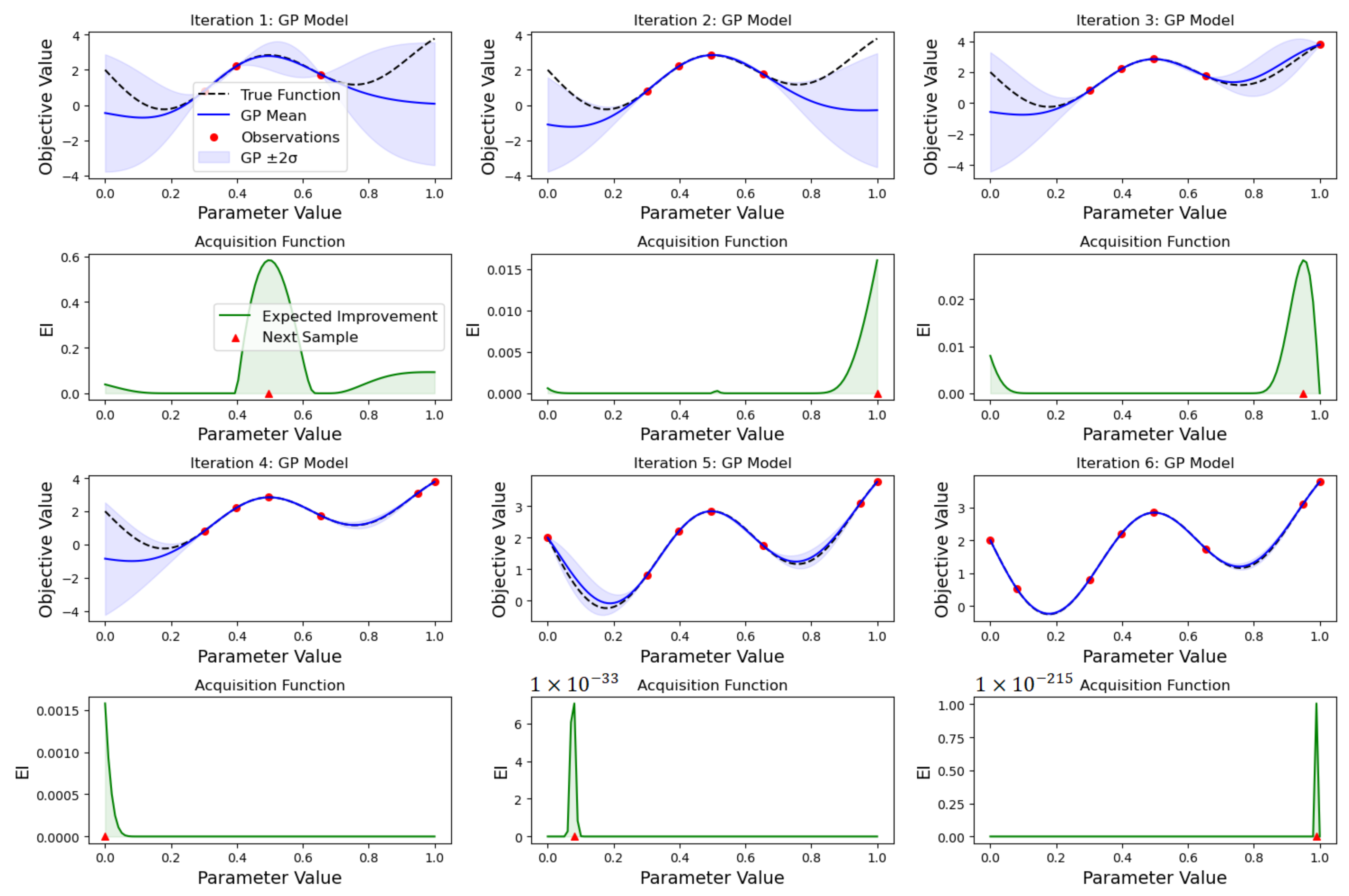
2.3.2. Bayesian Search

Bayesian Optimization (BO), more commonly known as Bayesian Search (BS), builds a surrogate model for optimizing the models [25]. Gaussian Process (GP) is commonly used because of its flexibility and strength. BO uses a surrogate model to approximate the objective function based on the observed data points [29]. Unlike GS and RS, BO uses an iteration approach to evaluate previously obtained results for future evaluation. This is carried out with an acquisition function that determines the next parameter to be evaluated. The Bayesian Optimization procedure is as follows:
  • Sampling the objective function at a few initial points.
  • Using the initial samples to build a surrogate model of the objective function.
  • Defining an acquisition function that uses the surrogate model to determine the next point to evaluate.
  • Evaluating the objective function at the point suggested by the acquisition function.
  • Updating the surrogate model with the new data point.
  • Repeating steps 3–5 until a stopping criterion is met.
Figure 2 below visualizes how Bayesian Optimization works through two main components: a surrogate model and an acquisition function.

2.4. Model Building

The predictive models built for this study were based on the Support Vector Machine (SVM), Random Forest (RF), and eXtreme Gradient Boosting (XGBoost) machine learning algorithms. In our previous review of 65 studies, these algorithms were found to be the most widely used for building predictive models [30]. They represent a traditional model (SVM), an ensemble model (RF), and a high-scalability model (XGBoost). We utilized a free version of Google Colab 1.2 to perform comparative analyses.
SVM is one of the most utilized traditional algorithms for both classification and regression predictive models [31,32]. As a supervised algorithm, SVM generates a hyperplane as a decision boundary for classification. Because our dataset has 2008 instances, it has 2008 data points. The objective function of SVM is as follows [7]:
arg min w 1 2008 i = 1 2008 max 0.1 y i f x i + C w T w
where C is the regularization parameter, and w is the normalization vector. These parameters are important for configuring SVM models. To obtain the optimal hyperplane for an SVM model, the decision function f x is defined as the function. This function measures the similarity between x i and x j , which can be of various types in SVM models. Consequently, the choice of the kernel type is crucial to tuning the hyper-parameter. Common kernel types in the SVM of this study include linear, radial basis function (RBF), and sigmoid kernels.
RF is commonly used for classification and regression purposes [33]. RF builds and trains multiple decision trees through a bagging method and combines the predictions made by the trees to obtain a more accurate and stable prediction [33,34]. RF is decision tree-based and has three essential components: a root node, decision nodes, and leaf nodes. In this study, we followed the hyper-parameters of RF as found in the scikit-learn library of Python 3.9 [7,35]. For more accurate decision-making, we configured the tree depth maximum to obtain a deeper tree. The decision and leaf nodes consist of sample split and leaf parameters that can be configured to prevent the model from overfitting possibility. Moreover, to control the number of features considered when looking for the best split at each node, we configured the maximum features parameter. Unlike Decision Tree (DT), RF has a parameter that controls the number of trees in a forest as n estimators, which we configured to determine the optimal decision trees of the model.
The other tree-based model is an XGBoost algorithm. This is a popular model that provides improved performance and speed through the use of boosting and gradient descent methods while combining decision trees [19,36]. We assigned additional parameters to our XGBoost model, including a learning rate that determines the boosting process, a subsample for the ratio of the training instances, and a colsample bytree that represents the subsample ratio while constructing decision trees.
Table 1 below lists the hyper-parameter configuration we tested to optimize the machine learning algorithms for our experimental setup, which is shown in Figure 3. The listed parameters are based on the algorithm’s characteristics.

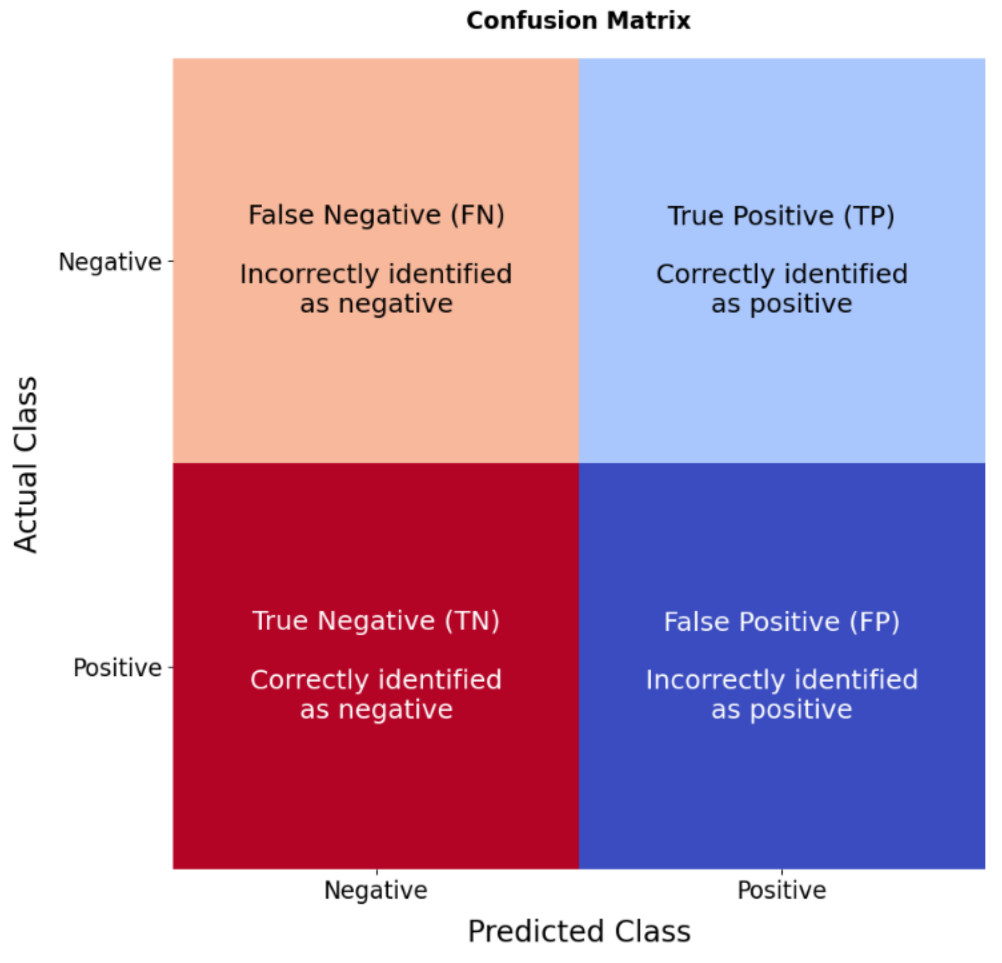
2.5. Model Evaluation

Evaluation of our models was carried out using classification metrics to calculate the accuracy, sensitivity, and AUC score of each model. Shown as a confusion matrix (Figure 4), classification metrics contain binary values of four prediction categories: true positives (TPs), false positives (FPs), true negatives (TNs), and false negatives (FNs) [37].
We divided the number of correct predictions (TP + TN) by the total number of predictions to obtain the accuracy of our models. Accuracy is the ratio of correctly predicted instances to the total instances and gives a straightforward measure of how often the model is correct [38].
A c c u r a c y = T P + T N T P + T N + F P + F N
We also measured the proportion of actual positives that were correctly identified by the model. This parameter is usually called sensitivity but also may be referred to as recall or True Positive Rate (TPR). To obtain this evaluation parameter, we divided the true positives (TP) by the sum of true positives (TP) and false negatives (FN) [37].
S e n s i t i v i t y = T P T P + F N
Moreover, we calculated the area under the curve (AUC), which represents the area under the Receiver Operating Characteristic (ROC) curve. This parameter is a performance metric for binary classification problems that plots the True Positive Rate (sensitivity) and the False Positive Rate (Specificity) at various threshold settings [39]. The AUC score ranges between 0 and 1.0, with an AUC of 0.5 suggesting no discrimination ability, meaning that the model’s performance is equivalent to random guessing and has no ability to discriminate between the positive and negative classes [40]. Figure 5 is an example of an AUC graph and its score.
To ensure robustness, we validated the models by stratified cross-validation with 10-fold [41], a variation in k-fold cross-validation stratified cross-validation that ensures that each fold is representative of the overall class distribution. Unlike regular n-fold cross-validation, stratification ensures that each fold has the same class distribution as the original dataset, providing a more accurate evaluation [42]. In this study, we calculated the AUC score for the cross-validation parameter to validate the possibility of underfitting in the models, which can be identified by comparing the AUC score of a baseline model with that of the 10-fold cross-validated model.

3. Results

For the comparisons of this study, 36 models were built with different pre-processing approaches and different hyper-parameter optimization methods. Each model was given the name of its algorithm and imputation technique. For example, the SVM-based model with mean imputation is referred to as SVM (Mean).

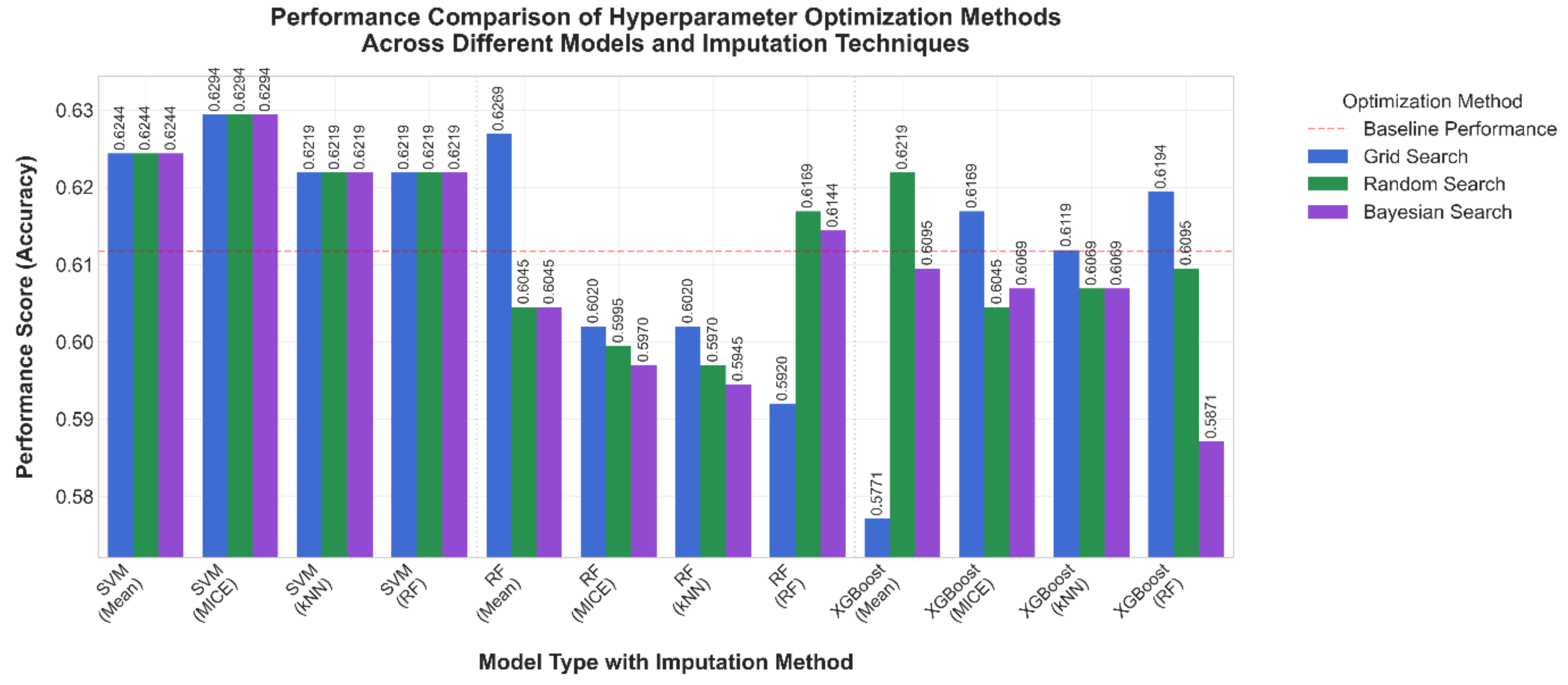
3.1. Comparative Results

Figure 6 is a comparison of the accuracy of our models, with the optimization method color-coded: Grid Search (blue), Random Search (green), and Bayesian search (purple). The baseline value is shown as a dashed line at approximately 0.611. Based on our experimental study, we found that the SVM model outperformed the other models, except for the pre-processing approach. The MICE imputation method with SVM yielded the highest accuracy, 0.6294, showing marginal effectiveness over the other imputation techniques. In contrast, RF, which underperformed the others, only displayed good performance when using mean imputation and Grid Search to determine the ideal configuration of its hyper-parameter, which ranged from 0.595 to 0.609. Unlike SVM and RF, the XGBoost models achieved varying levels of accuracy based on the imputation technique, between 0.577 and 0.619.
Figure 7 shows the sensitivity of each model. The baseline performance, approximately 0.575, is shown as a dashed line. The SVM models consistently demonstrated superior performance across all imputation methods, achieving sensitivity scores above 0.61. Notably, performance was consistent across all three optimization methods, with minimal variation of less than 0.005. The RF models showed sensitivity scores ranging from 0.52 to 0.60, while XGBoost models achieved intermediate performance levels of 0.55 and 0.59. Examination of the imputation methods showed that MICE resulted in marginally higher sensitivity scores compared to mean imputation, with improvements of approximately 0.002–0.005 across most models.
A comparison of the AUC scores is shown in Figure 8. As with the other performance comparisons, the SVM models consistently demonstrated superior performance, achieving AUC scores exceeding 0.66 across all the imputation methods. They remained stable across the optimization methods, with a variation of less than 0.001. The RF models exhibited AUC scores ranging from 0.60 to 0.63, while the XGBoost models achieved intermediate performance levels between 0.61 and 0.65. MICE showed marginally higher AUC scores than the other imputation methods, with improvements ranging from 0.001 to 0.003 across most model configurations when compared to mean imputation.

3.2. Comparison After 10-Fold Cross Validation

We validated the proposed models by 10-fold cross-validation with the AUC score as the validation parameter. Figure 9 shows a comparison of the average AUC scores of all proposed models after 10-fold cross-validation. Distinct performance patterns were found in terms of the average AUC score after 10-fold cross-validation. The SVM models achieved the best performance, with an average AUC score of around 0.652 across all imputation techniques. The RF models showed more variable performance, with the average AUC score ranging from 0.645 to 0.663, notably achieving the highest score when paired with mean imputation and Bayesian Search optimization. The XGBoost models demonstrated scores between 0.638 and 0.662, with Random Search optimization generally yielding better results than the other optimization methods.

3.3. Optimized Hyper-Parameter

Through our three optimization methods, we obtained optimized hyper-parameters for each of our models, as shown in Table 2. The three optimization methods for SVM were configured with the same hyper-parameter, indicating that they would be ideal for SVM applications to this type of dataset. In contrast, both RF and XGBoost showed different hyper-parameters. For the RF models, Grid Search optimization generated a “True” value across all the imputation techniques, while Bayesian Search generated a “False” value for their bootstrap parameter. The XGBoost models were similar in that in their Grid Search optimization, the learning rates were more than 0.1, while in Random Search, the XGBoost models had a learning rate of 0.01 across all the imputation techniques.
Furthermore, we calculated the processing time of each model for each optimization method for comparison. In this study, we used a free version of Google Colab with an Intel Xeon CPU (Santa Clara, CA, USA) with two virtual CPUs and 13GB of RAM as its default CPU that runs on a laptop computer with an Intel i5 processor, 8GB of RAM, and without an external CPU. Although the processing time would differ from other computer software and hardware, our comparison provides valuable insights into hyper-parameter optimization on machine learning-based models.
Table 3 shows the average processing time of each model according to the optimization method. We found that Grid Search optimization consumed more processing time than other optimization methods, while Bayesian Search provided the fastest processing time. Optimization with SVM required more time than the other proposed algorithms, approximately 9.7 min on average for each model, with RF 6.27 min and XGBoost 5.6 min.

4. Discussion

This comparative analysis yielded several significant insights into the relationship between various approaches to model selection, imputation strategy, and hyper-parameter optimization. In our initial models, SVM outperformed the other models in terms of accuracy, sensitivity, and AUC score and demonstrated consistent performance across all three metrics. The SVM models maintained scores for accuracy above 0.62, with MICE imputation showing the best results (0.6294). The SVM models had consistently high AUC scores (0.62–0.66), and similarly, the models achieved sensitivity scores above 0.61. The simple characteristics of the SVM models make it attractive for applications where consistent performance is crucial [31,32]; however, after 10-fold cross-validation, the AUC scores of the SVM models were slightly reduced, indicating the possibility of overfitting. The differences between the initial SVM models and those after 10-fold cross-validation averaged −0.0074. Although not significant, the declines indicate that the models were not sufficiently robust to handle the various features of the dataset [23,24].
The RF models exhibited a more variable performance pattern across the three optimization methods. While they showed moderate accuracy (0.595–0.609), their AUC scores demonstrated interesting behavior, achieving the highest score (0.663) when used with Mean Imputation and Bayesian Search optimization. However, their sensitivity scores were notably lower (0.52–0.56), indicating potential issues with identifying positive cases [37]. This variability indicates that RF models require careful consideration of the selection of both the imputation technique and optimization strategy, with performance heavily dependent on these choices. Interestingly, the RF models showed behavioral changes between the initial and cross-validated scenarios. After cross-validation, the RF models presented performance improvements in some configurations in terms of AUC score, reaching approximately 0.663. Inversely proportional to the SVM models, the RF models provided enhancement in terms of AUC score after 10-fold cross-validation, an average increase of 0.03815, which indicates that they are more robust than SVM models.
The XGBoost models presented the most complex performance profile among the three algorithms. Their accuracy showed high variability, with scores ranging between 0.577 and 0.619, and they performed very competitively in terms of AUC, from 0.638 to 0.662, with Random Search optimization generally yielding the best results. The XGBoost models revealed moderate performance for sensitivity (0.56–0.58), and they had a strong response to the optimization method, particularly Random Search, across all methods. This finding suggests that XGBoost’s hyper-parameter landscape might be better suited to exploration through random sampling rather than systematic or Bayesian approaches. Unlike the initial XGBoost models, after 10-fold cross-validation, they became more consistent, achieving scores of 0.655–0.658. Even though there was a decline of 0.0101 when incorporating RF imputation and Grid Search optimization, the other XGBoost models presented an average improvement of 0.01683. This improvement indicates that the XGBoost models have the possibility of maintaining predictive performance while handling various features in a dataset [41]. The improvements in these models were not better than those of the RF models (+0.03815) but were better than those of the SVM models (−0.0074). Compared to our XGBoost models, the current models showed significant improvement in every aspect of the performance parameters, indicating that this optimization method works well in improving predictive performance [19].
MICE generally showed slight advantages over the SVM models in terms of mean imputation, while the pattern was less clear for the RF and XGBoost models. MICE imputation showed consistent performance across all models, but due to its complexity, it did not provide the expected advantages over simpler methods like mean imputation [19]. After cross-validation, the XGBoost models worked better than the others with kNN imputation, while RF imputation showed variable results across all models.
The effectiveness of the optimization methods varied by model type. The SVM models presented minimal variation across the optimization methods, suggesting that the model’s hyper-parameter space might be relatively smooth and well-behaved due to its less complex characteristics. The RF models benefited more from Bayesian Search but showed a preference for Random Search, particularly after cross-validation. XGBoost showed better results with Random Search and generally outperformed Grid Search, especially in cross-validated scenarios. These findings suggest that the choice of optimization method should be model-specific rather than follow a one-size-fits-all approach.
We used cross-validation to provide a more realistic assessment of model performance and generalization capabilities [42]. This generated several important insights, including that some configurations that performed well in baseline testing showed decreased performance under cross-validation, which indicates potential overfitting in the baseline models. On the other hand, the RF and XGBoost models showed increased performance under cross-validation, which suggests they are more robust and reliable.
In general, the findings of this study suggest that even though model choice is essential, the selection of an appropriate hyper-parameter optimization method and imputation technique can have significant impacts on model performance. The results also emphasize the importance of cross-validation to obtain reliable performance estimates: baseline performance metrics alone may not provide a complete picture of model generalization capability. Additionally, Bayesian Search consistently required less processing time compared to Grid and Random Search in terms of computational efficiency, with average processing times of 7, 5.3, and 4.8 min, respectively, for SVM, RF, and XGBoost. The software and hardware that were used to conduct these experimental studies have limits to their processing ability. Thus, processing times would differ with other devices.
Although our study primarily focuses on comparing hyper-parameter optimization methods and used metrics such as accuracy, sensitivity, and AUC, the clinical context of heart failure prediction remains an important consideration. In practice, predictive models must not only deliver robust statistical performance but also offer interpretability and reliable decision thresholds that balance sensitivity and specificity—key aspects for clinical decision-making [4,6]. For instance, while our SVM model achieved high-performance metrics, the slight overfitting observed during cross-validation underscores the need for future work to integrate interpretability techniques and threshold calibration to minimize misclassification risks. These enhancements would help bridge the gap between methodological optimization and practical, clinically deployable tools, ultimately supporting more informed decisions in patient management [7].
This study has limitations, including the generalizability of the dataset we used in this experiment. We only relied on a dataset from a single hospital (Zigong Fourth People’s Hospital, China), which may limit the generalizability of our findings. We used Google Colab with limited computational resources and a laptop with an Intel i5 processor (Santa Clara, CA, USA) and 8GB of RAM for the model building and evaluations, which may have impacted the depth of our optimization and model evaluation. Furthermore, because we focused more on the optimization comparative analysis than on the validation of the models, we did not include an external dataset for external validation. However, these limitations lead to our future work improving the depth of the validation of our models.

5. Conclusions

This comprehensive, comparative study used an electronic health records-based dataset from real patients and demonstrated that the optimization of predictive models leads to their ideal configuration for the prediction of the risk of heart failure. Our initial SVM models demonstrated excellent performance but had overfitting issues after 10-fold cross-validation, with an average AUC score decline of 0.0074. In contrast, our RF models offered remarkable improvement after cross-validation (+0.03815 AUC), specifically when mean imputation and Bayesian Search optimization were included, indicating robust generalization capabilities. Similarly, XGBoost models exhibited moderate improvement (+0.01683 AUC) and worked well with Random Search optimization.
Future studies will be necessary to explore the computational efficiency trade-offs inherent to these approaches and to investigate their performance stability across different types of datasets and missing data patterns. Additionally, examining the interactions between these methods and different types of data distribution will provide valuable insights for model selection in specific domains. Moreover, model interpretability, threshold optimization, and a detailed clinical use-case scenario are important future directions.

Author Contributions

Conceptualization, Q.A.H. and E.H.; methodology, Q.A.H.; writing—original draft preparation, Q.A.H.; software, Q.A.H.; validation, Q.A.H. and E.H.; writing—review and editing, Q.A.H. and E.H.; supervision, E.H. All authors have read and agreed to the published version of the manuscript.

Funding

This research received no external funding.

Institutional Review Board Statement

This study used a dataset from Physionet that is publicly accessible but has restricted access to download. This study was conducted in accordance with the Declaration of Helsinki and approved by the Institutional Review Board of Zigong Fourth People’s Hospital (protocol code: 2020-010 and day of approval: 8 June 2020).

Informed Consent Statement

Not applicable.

Data Availability Statement

The dataset used in this study can be accessed at https://physionet.org/content/heart-failure-zigong/1.3/ (accessed on 17 December 2024).

Acknowledgments

The authors would like to thank the Laboratory of Fundamental and Applied Informatics at Saga University, who supported this study.

Conflicts of Interest

The authors declare no conflicts of interest.

References

  1. Khan, M.S.; Shahid, I.; Bennis, A.; Rakisheva, A.; Metra, M.; Butler, J. Global Epidemiology of Heart Failure. Nat. Rev. Cardiol. 2024, 21, 717–734. [Google Scholar] [CrossRef] [PubMed]
  2. Zhao, H.; Liu, Z.; Li, M.; Liang, L. Optimal Monitoring Policies for Chronic Diseases under Healthcare Warranty. Socio-Econ. Plan. Sci. 2022, 84, 101384. [Google Scholar] [CrossRef]
  3. Badawy, M.; Ramadan, N.; Hefny, H.A. Healthcare Predictive Analytics Using Machine Learning and Deep Learning Techniques: A Survey. J. Electr. Syst. Inf. Technol. 2023, 10, 40. [Google Scholar] [CrossRef]
  4. Landicho, J.A.; Esichaikul, V.; Sasil, R.M. Comparison of Predictive Models for Hospital Readmission of Heart Failure Patients with Cost-Sensitive Approach. Int. J. Healthc. Manag. 2021, 14, 1536–1541. [Google Scholar] [CrossRef]
  5. Plati, D.K.; Tripoliti, E.E.; Bechlioulis, A.; Rammos, A.; Dimou, I.; Lakkas, L.; Watson, C.; McDonald, K.; Ledwidge, M.; Pharithi, R.; et al. A Machine Learning Approach for Chronic Heart Failure Diagnosis. Diagnostics 2021, 11, 1863. [Google Scholar] [CrossRef]
  6. Li, F.; Xin, H.; Zhang, J.; Fu, M.; Zhou, J.; Lian, Z. Prediction Model of In-hospital Mortality in Intensive Care Unit Patients with Heart Failure: Machine Learning-Based, Retrospective Analysis of the MIMIC-III Database. BMJ Open 2021, 11, e044779. [Google Scholar] [CrossRef]
  7. Bischl, B.; Binder, M.; Lang, M.; Pielok, T.; Richter, J.; Coors, S.; Thomas, J.; Ullmann, T.; Becker, M.; Boulesteix, A.; et al. Hyperparameter Optimization: Foundations, Algorithms, Best Practices, and Open Challenges. WIREs Data Min. Knowl. 2023, 13, e1484. [Google Scholar] [CrossRef]
  8. Fernando, T.; Gammulle, H.; Denman, S.; Sridharan, S.; Fookes, C. Deep Learning for Medical Anomaly Detection—A Survey. ACM Comput. Surv. 2022, 54, 3464423. [Google Scholar] [CrossRef]
  9. Patil, S.; Bhosale, S. Hyperparameter Tuning Based Performance Analysis of Machine Learning Approaches for Prediction of Cardiac Complications. In Proceedings of the 12th International Conference on Soft Computing and Pattern Recognition (SoCPaR 2020), Virtual, 15–18 December 2020; Advances in Intelligent Systems and Computing. Abraham, A., Ohsawa, Y., Gandhi, N., Jabbar, M.A., Haqiq, A., McLoone, S., Issac, B., Eds.; Springer International Publishing: Cham, Switzerland, 2021; Volume 1383, pp. 605–617, ISBN 978-3-030-73688-0. [Google Scholar]
  10. Firdaus, F.F.; Nugroho, H.A.; Soesanti, I. Deep Neural Network with Hyperparameter Tuning for Detection of Heart Disease. In Proceedings of the 2021 IEEE Asia Pacific Conference on Wireless and Mobile (APWiMob), Bandung, Indonesia, 8 April 2021; pp. 59–65. [Google Scholar]
  11. Belete, D.M.; Huchaiah, M.D. Grid Search in Hyperparameter Optimization of Machine Learning Models for Prediction of HIV/AIDS Test Results. Int. J. Comput. Appl. 2022, 44, 875–886. [Google Scholar] [CrossRef]
  12. Asif, D.; Bibi, M.; Arif, M.S.; Mukheimer, A. Enhancing Heart Disease Prediction through Ensemble Learning Techniques with Hyperparameter Optimization. Algorithms 2023, 16, 308. [Google Scholar] [CrossRef]
  13. Valarmathi, R.; Sheela, T. Heart Disease Prediction Using Hyper Parameter Optimization (HPO) Tuning. Biomed. Signal Process. Control 2021, 70, 103033. [Google Scholar] [CrossRef]
  14. Sharma, N.; Malviya, L.; Jadhav, A.; Lalwani, P. A Hybrid Deep Neural Net Learning Model for Predicting Coronary Heart Disease Using Randomized Search Cross-Validation Optimization. Decis. Anal. J. 2023, 9, 100331. [Google Scholar] [CrossRef]
  15. Gao, L.; Ding, Y. Disease Prediction via Bayesian Hyperparameter Optimization and Ensemble Learning. BMC Res. Notes 2020, 13, 205. [Google Scholar] [CrossRef] [PubMed]
  16. Liu, X.; Wu, Y.; Wu, H. Machine Learning Enabled 3D Body Measurement Estimation Using Hybrid Feature Selection and Bayesian Search. Appl. Sci. 2022, 12, 7253. [Google Scholar] [CrossRef]
  17. Zhang, Z.; Cao, L.; Chen, R.; Zhao, Y.; Lv, L.; Xu, Z.; Xu, P. Electronic Healthcare Records and External Outcome Data for Hospitalized Patients with Heart Failure. Sci. Data 2021, 8, 46. [Google Scholar] [CrossRef]
  18. Zhang, Z.; Cao, L.; Zhao, Y.; Xu, Z.; Chen, R.; Lv, L.; Xu, P. Hospitalized Patients with Heart Failure: Integrating Electronic Healthcare Records and External Outcome Data. PhysioNet 2020, 101, e215–e220. [Google Scholar] [CrossRef]
  19. Hidayaturrohman, Q.A.; Hanada, E. Impact of Data Pre-Processing Techniques on XGBoost Model Performance for Predicting All-Cause Readmission and Mortality Among Patients with Heart Failure. BioMedInformatics 2024, 4, 2201–2212. [Google Scholar] [CrossRef]
  20. Psychogyios, K.; Ilias, L.; Ntanos, C.; Askounis, D. Missing Value Imputation Methods for Electronic Health Records. IEEE Access 2023, 11, 21562–21574. [Google Scholar] [CrossRef]
  21. Dahouda, M.K.; Joe, I. A Deep-Learned Embedding Technique for Categorical Features Encoding. IEEE Access 2021, 9, 114381–114391. [Google Scholar] [CrossRef]
  22. Sinsomboonthong, S. Performance Comparison of New Adjusted Min-Max with Decimal Scaling and Statistical Column Normalization Methods for Artificial Neural Network Classification. Int. J. Math. Math. Sci. 2022, 2022, 3584406. [Google Scholar] [CrossRef]
  23. Pei, X.; Zhao, Y.H.; Chen, L.; Guo, Q.; Duan, Z.; Pan, Y.; Hou, H. Robustness of Machine Learning to Color, Size Change, Normalization, and Image Enhancement on Micrograph Datasets with Large Sample Differences. Mater. Des. 2023, 232, 112086. [Google Scholar] [CrossRef]
  24. Pfob, A.; Lu, S.-C.; Sidey-Gibbons, C. Machine Learning in Medicine: A Practical Introduction to Techniques for Data Pre-Processing, Hyperparameter Tuning, and Model Comparison. BMC Med. Res. Methodol. 2022, 22, 282. [Google Scholar] [CrossRef] [PubMed]
  25. Priyadarshini, I.; Cotton, C. A Novel LSTM–CNN–Grid Search-Based Deep Neural Network for Sentiment Analysis. J Supercomput. 2021, 77, 13911–13932. [Google Scholar] [CrossRef] [PubMed]
  26. Bergstra, J.; Bengio, Y. Random Search for Hyper-Parameter Optimization. J. Mach. Learn. Res. 2012, 13, 281–305. [Google Scholar]
  27. Ali, Y.; Awwad, E.; Al-Razgan, M.; Maarouf, A. Hyperparameter Search for Machine Learning Algorithms for Optimizing the Computational Complexity. Processes 2023, 11, 349. [Google Scholar] [CrossRef]
  28. Tunçel, M.; Duran, A. Effectiveness of Grid and Random Approaches for a Model Parameter Vector Optimization. J. Comput. Sci. 2023, 67, 101960. [Google Scholar] [CrossRef]
  29. Bahan Pal, J.; Mj, D. Improving Multi-Scale Attention Networks: Bayesian Optimization for Segmenting Medical Images. Imaging Sci. J. 2023, 71, 33–49. [Google Scholar] [CrossRef]
  30. Hidayaturrohman, Q.A.; Hanada, E. Predictive Analytics in Heart Failure Risk, Readmission, and Mortality Prediction: A Review. Cureus 2024, 16, e73876. [Google Scholar] [CrossRef]
  31. Hearst, M.A.; Dumais, S.T.; Osuna, E.; Platt, J.; Scholkopf, B. Support Vector Machines. IEEE Intell. Syst. Their Appl. 1998, 13, 18–28. [Google Scholar] [CrossRef]
  32. Chen, Y.; Mao, Q.; Wang, B.; Duan, P.; Zhang, B.; Hong, Z. Privacy-Preserving Multi-Class Support Vector Machine Model on Medical Diagnosis. IEEE J. Biomed. Health Inform. 2022, 26, 3342–3353. [Google Scholar] [CrossRef]
  33. Manzali, Y.; Elfar, M. Random Forest Pruning Techniques: A Recent Review. Oper. Res. Forum 2023, 4, 43. [Google Scholar] [CrossRef]
  34. Breiman, L. Random Forests. Mach. Learn. 2001, 45, 5–32. [Google Scholar] [CrossRef]
  35. Pedregosa, F.; Varoquaux, G.; Gramfort, A.; Michel, V.; Thirion, B.; Grisel, O.; Blondel, M.; Prettenhofer, P.; Weiss, R.; Dubourg, V.; et al. Scikit-Learn: Machine Learning in Python. J. Mach. Learn. Res. 2011, 12, 2825–2830. [Google Scholar]
  36. Chen, T.; Guestrin, C. XGBoost: A Scalable Tree Boosting System. In Proceedings of the Proceedings of the 22nd ACM SIGKDD International Conference on Knowledge Discovery and Data Mining, San Francisco, CA, USA, 13 August 2016; pp. 785–794.
  37. Vujovic, Ž.Ð. Classification Model Evaluation Metrics. Int. J. Adv. Comput. Sci. Appl. 2021, 12, 599–606. [Google Scholar] [CrossRef]
  38. Ali, M.M.; Paul, B.K.; Ahmed, K.; Bui, F.M.; Quinn, J.M.W.; Moni, M.A. Heart Disease Prediction Using Supervised Machine Learning Algorithms: Performance Analysis and Comparison. Comput. Biol. Med. 2021, 136, 104672. [Google Scholar] [CrossRef]
  39. Zhang, Y.; Gao, Z.; Wittrup, E.; Gryak, J.; Najarian, K. Increasing Efficiency of SVMp+ for Handling Missing Values in Healthcare Prediction. PLoS Digit. Health 2023, 2, e0000281. [Google Scholar] [CrossRef]
  40. Chen, S.; Hu, W.; Yang, Y.; Cai, J.; Luo, Y.; Gong, L.; Li, Y.; Si, A.; Zhang, Y.; Liu, S.; et al. Predicting Six-Month Re-Admission Risk in Heart Failure Patients Using Multiple Machine Learning Methods: A Study Based on the Chinese Heart Failure Population Database. J. Clin. Med. 2023, 12, 870. [Google Scholar] [CrossRef]
  41. Bates, S.; Hastie, T.; Tibshirani, R. Cross-Validation: What Does It Estimate and How Well Does It Do It? J. Am. Stat. Assoc. 2024, 119, 1434–1445. [Google Scholar] [CrossRef]
  42. Lasfar, R.; Tóth, G. The Difference of Model Robustness Assessment Using Cross-validation and Bootstrap Methods. J. Chemom. 2024, 38, e3530. [Google Scholar] [CrossRef]
Figure 1. Grid Search and Random Search.
Applsci 15 03393 g001
Figure 2. Bayesian Optimization.
Applsci 15 03393 g002
Figure 3. Experimental flow chart [17].
Applsci 15 03393 g003
Figure 4. Confusion matrix used for classification metrics.
Applsci 15 03393 g004
Figure 5. Receiver Operating Characteristic curve example.
Applsci 15 03393 g005
Figure 6. Comparison of the accuracy of our 36 models.
Applsci 15 03393 g006
Figure 7. Comparison of the sensitivity of our 36 models.
Applsci 15 03393 g007
Figure 8. Comparison of the AUC scores of our 36 models.
Applsci 15 03393 g008
Figure 9. Comparison of the average AUC score after 10-fold cross-validation.
Applsci 15 03393 g009
Table 1. List of configurations for the hyper-parameter of the algorithms.
AlgorithmHyper-ParameterValues
Support Vector MachineC0.1, 1.0, 10, 100, 1000
Gamma1, 0.1, 0.01, 0.001, 0.0001, auto, scale
KernelLinear, RBF, Sigmoid
Random ForestBootstrapTrue, False
Max depth10, 20, 30, None
Max feature2, 3
Min samples leaf3, 4, 5
Min sample split2, 5, 10
N-estimators100, 200, 300, 500
XGBoostMax depth3, 5, 7, 10
Learning rate0.2, 0.15, 0.1, 0.01, 0.001
Subsample0.5, 0.7, 1.0
N-estimators50, 100, 150, 200, 300
Colsample bytree0.5, 0.7, 1.0
Table 2. Optimized hyper-parameters with the Grid, Random, and Bayesian Searches.
ModelOptimized Parameters
AlgorithmImputationGrid SearchRandom SearchBayesian Search
SVMMeanC = 1; gamma = 0.01; kernel = RBFC = 1; gamma = 0.01; kernel = RBFC = 1; gamma = 0.01; kernel = RBF
MICEC = 1; gamma = 0.01; kernel = RBFC = 1; gamma = 0.01; kernel = RBFC = 1; gamma = 0.01; kernel = RBF
kNNC = 1; gamma = auto; kernel = RBFC = 1; gamma = auto; kernel = RBFC = 1; gamma = auto; kernel = RBF
RFC = 1; gamma = 0.01; kernel = RBFC = 1; gamma = 0.01; kernel = RBFC = 1; gamma = 0.01; kernel = RBF
RFMeanbootstrap = True; max depth = 20; max feature = 3; min samples leaf = 3; min samples split = 5; n_estimators = 300bootstrap = False; max depth = 20; max features = 3; min samples leaf = 3; min samples split = 5; n_estimators = 200bootstrap = False; max depth = 20; max features = 3; min samples leaf = 4; min samples split = 5; n_estimators = 300
MICEbootstrap = True; max depth = 20; max feature = 3; min samples leaf = 4; min samples split = 10; n_estimators = 300bootstrap = True; max depth = None; max features = 3; min samples leaf = 3; min samples split = 10; n_estimators = 300bootstrap = False; max depth = 20; max features = 3; min samples leaf = 3; min samples split = 2; n_estimators = 200
kNNbootstrap = True; max depth = 20; max feature = 2; min samples leaf = 3; min samples split = 10; n_estimators = 300bootstrap = False; max depth = 20; max features = 3; min samples leaf = 4; min samples split = 10; n_estimators = 500bootstrap = False; max depth = 20; max features = 3; min samples leaf = 4; min samples split = 2; n_estimators = 300
RFbootstrap = True; max depth = 20; max feature = 2; min samples leaf = 3; min samples split = 5; n_estimators = 300bootstrap = False; max depth = None; max feature = 2; min samples leaf = 3; min samples split = 5; n_estimators = 200bootstrap = False; max depth = 30; max feature = 3; min samples leaf = 5; min samples split = 10; n_estimators = 300
XGBoostMeanlearning rate = 0.2; max depth = 7; subsample = 1; colsample_bytree = 1; n_estimators = 100learning rate = 0.01; max depth = 10; subsample = 0.7; colsample_bytree = 0.7; n_estimators = 300learning rate = 0.01; max depth = 7; subsample = 0.7; colsample_bytree = 0.5; n_estimators = 150
MICElearning rate = 0.15; max depth = 7; subsample = 0.5; colsample_bytree = 1; n_estimators = 100learning rate = 0.01; max depth = 10; subsample = 0.7; colsample_bytree = 1; n_estimators = 300learning rate = 0.01; max depth = 10; subsample = 0.7; colsample_bytree = 0.5; n_estimators = 300
kNNlearning rate = 0.1; max depth = 7; subsample = 0.5; colsample_bytree = 1; n_estimators = 100learning rate = 0.01; max depth = 10; subsample = 0.5; colsample_bytree = 1; n_estimators = 300learning rate = 0.01; max depth = 10; subsample = 0.5; colsample_bytree = 1; n_estimators = 300
RFlearning rate = 0.1; max depth = 5; subsample = 1; colsample_bytree = 1; n_estimators = 100learning rate = 0.01; max depth = 7; subsample = 0.5; colsample_bytree = 0.7; n_estimators = 200learning rate = 0.1; max depth = 5; subsample = 0.7; colsample_bytree = 0.7; n_estimators = 50
Table 3. Approximate processing time with hyper-parameter optimization.
Optimization MethodAlgorithmAverage Processing Time per Model (Min)
Grid SearchSVM12
RF7
XGBoost6
Random SearchSVM10
RF6.5
XGBoost6
Bayesian SearchSVM7
RF5.3
XGBoost4.8
Disclaimer/Publisher’s Note: The statements, opinions and data contained in all publications are solely those of the individual author(s) and contributor(s) and not of MDPI and/or the editor(s). MDPI and/or the editor(s) disclaim responsibility for any injury to people or property resulting from any ideas, methods, instructions or products referred to in the content.

