Article

Conditional GAN-Based Two-Stage ISP Tuning Method: A Reconstruction–Enhancement Proxy Framework

School of Information Science and Engineering, East China University of Science and Technology, Shanghai 200237, China
*
Author to whom correspondence should be addressed.
Appl. Sci. 2025, 15(6), 3371; https://doi.org/10.3390/app15063371
Submission received: 3 March 2025 / Revised: 17 March 2025 / Accepted: 18 March 2025 / Published: 19 March 2025
(This article belongs to the Special Issue Application of Artificial Intelligence in Image Processing)

Abstract

:
Image signal processing (ISP), a critical component in camera imaging, has traditionally relied on experience-driven parameter tuning. This approach suffers from inefficiency, fidelity issues, and conflicts with visual enhancement objectives. This paper introduces ReEn-GAN, an innovative staged ISP proxy tuning framework. ReEn-GAN decouples the ISP process into two distinct stages: reconstruction (physical signal recovery) and enhancement (visual quality and color optimization). By employing distinct network architectures and loss functions tailored to specific objectives, the two-stage proxy can effectively optimize both the reconstruction and enhancement modules within the ISP pipeline. Compared to tuning with an end-to-end proxy network, the proposed method’s proxy more effectively extracts hierarchical information from the ISP pipeline, thereby mitigating the significant changes in image color and texture that often result from parameter adjustments in an end-to-end proxy model. This paper conducts experiments on image denoising and object detection tuning tasks, and compares the performance of the two types of proxies. The results demonstrate that the proposed method outperforms end-to-end proxy methods on public datasets (SIDD, KITTI) and achieves over 21% improvement in performance metrics compared to hand-tuning methods.

1. Introduction

In modern image processing systems, the image signal processor (ISP) transforms the raw signals captured by image sensors into image signals comprehensible to both human eyes and machines. Modern ISPs consist of numerous independent yet interconnected modules. These modules sequentially convert the raw signals into image signals, while also processing and optimizing the image information to better align with human visual requirements or machine vision needs. During their design, these modules adhere to the principle of divide and conquer, breaking down the image processing tasks into distinct steps. Each critical step handles specific image processing tasks, including demosaicing, noise reduction, white balance, and color correction. Through the pipeline of all modules within the ISP, the image undergoes processing and optimization [1].
On the one hand, the image processing effect of each module in the ISP is not constant [2]. Modern ISPs need to adjust the algorithm for different scenes. The adjustment here is more about the optimization of the algorithm itself than the optimization of the ISP pipeline. In order to make the ISP adapt to more scenarios and obtain better adaptability, modern ISPs usually expose many super parameters and configuration interfaces of the algorithm to the outside world, so that the algorithm can adapt to more scenarios. In the actual development scenario, professional image tuning experts will coordinate the ISP and the entire image acquisition system (including cameras, image sensors, ISP and back-end processing), and set the optimal parameter set for the ISP in different scenarios. This process is time-consuming, and it is difficult to obtain the optimal parameter set for the scene, and the process of tuning is subject to the experience and subjective evaluation of tuning experts.
On the other hand, ISP output images are not only used for Human Visions (HV). In many scenarios, ISP output images are often used for Computer Vision (CV) tasks such as image recognition, image segmentation [3], etc. Under the traditional ISP tuning method, the goal of tuning is mainly based on the subjective evaluation of image tuning experts [4] and some commonly used image quality standards [5,6,7,8]. These image quality standards cannot strictly correspond to downstream tasks. The excellence of the image quality standard does not mean that the accuracy of the CV task is high, and the traditional image tuning cannot carry out specific tuning for the CV task [9], which leads to a certain impact on the accuracy of the CV task when ISP is used for some downstream tasks [10,11].
Therefore, the method of tuning for CV tasks not based on tuning experts is gradually emerging [12]. To facilitate the feedback of CV task losses to the ISP tuning system, an agent-based ISP tuning approach is employed. This method fits the ISP pipeline using a differentiable network, allowing the loss from downstream tasks to be backpropagated to the input parameters of the proxy ISP. This enables parameter adjustments tailored to specific tasks. Subsequently, the tuned parameters are passed to the hardware ISP, achieving optimal parameter configuration for the ISP.
The existing proxy-based ISP tuning methods came from end-to-end proxy training methods [13]. The advantage of the end-to-end proxy method lies in the fact that the proxy network can capture the sequential effects of all levels of modules in the ISP pipeline on image processing. However, due to the complexity of the ISP pipeline, a single network often fails to distinguish the optimization objectives of different type modules, resulting in conflicts in optimization directions. This paper utilizes the different optimization objectives of different type modules in the ISP pipeline [14] and proposes a two-stage ISP proxy tuning method based on reconstruction and enhancement, thus avoiding the tuning interference and parameter search difficulties caused by end-to-end approaches.
In this paper, our contributions can be summarized as follows:
1.
Propose ReEn-GAN and build an AI-assisted ISP tuning process for CV tasks based on a proxy method. The system uses ReEn-GAN as a two-stage proxy to fit the entire ISP and its parameters, and reversely optimizes the proxy parameters through the evaluation indicators of CV tasks and applies them to the existing ISP, greatly simplifying the process of manual tuning ISP;
2.
Utilize the prior knowledge of ISP to decompose the ISP pipeline into two processes: reconstruction and enhancement. By using an alternating network structure and loss functions of the two-stage proxies, the problems of significant changes in image color and texture that result from parameter adjustments, parameter interference and proxy training difficulties in the end-to-end proxy method are solved;
3.
Verify the feasibility of using ReEn-GAN for auto-tuning in CV scenes such as image denoising and object detection, as well as the impact of different loss functions and pyramid pooling module (PPM) additions on proxy tuning performance.
The remaining sections of this paper are organized as follows: Section 2 provides an overview of related works on ISP tuning, including proxy-based tuning methods and other algorithms in CV-oriented ISP optimization. Section 3 provides a detailed introduction to the tuning process and the architecture of ReEn-GAN proposed in this paper. Section 4 presents the results of various experiments conducted to evaluate the performance of the proposed method. Finally, Section 5 summarizes the main contributions of this paper.

2. Related Works

In this section, we will discuss the significance of module tuning in the ISP pipeline and the research progress of global automatic tuning.
In order to achieve the control of multiple image processing tasks and adaptive sensors, modern hardware ISPs often divide image processing tasks into independent image processing modules [1], which independently or jointly process some image tasks such as image domain conversion, white balance processing, image noise reduction, distortion correction, automatic exposure, automatic focusing, etc. The modules are processed in order to form an ISP pipeline.
In order to reduce the cost of ISP tuning and minimize the impact of subjective human feelings on downstream tasks, many efforts have been focused on ISP auto-tuning in recent years. Due to the fact that hyper-parameter optimization for CV tasks generally has clear loss values, traditional auto-tuning methods mainly use random search [15] and other methods to find hyper-parameters for CV systems. At the same time, as ISP manufacturers gradually protect their ISP’s specific IP information, users become blind to the specific algorithms in hardware ISPs, making ISPs a black box to the outside world. Some optimization methods for specific image performance indicators gradually become more complex. Subsequently, with the improvement of computer performance, the popularity of proxy neural networks, and the increasing complexity of image metrics, the development of ISP auto-tuning has gradually diverged in two dimensions.
One dimension is whether ISP is seen as a black box. Treating ISP as a black box [13] means that for high-level tuning algorithms, there is no essential difference between parameters. Using the same method for tuning is beneficial for eliminating the influence between modules and parameters. If ISP is not seen as a black box [16], then the tuning algorithm will more explicitly adjust the parameters of ISP, which will be more targeted to the ISP structure, but there may be difficulties in achieving the Pareto front.
Another dimension is whether the tuning process uses some proxy method to simulate the functionality of the ISP. In the method of using proxy [17], the entire ISP is fitted into a differentiable model through a certain algorithm. By using gradient descent in the parameter space of the model, the optimal parameter set is found and applied to the hardware ISP. The non-proxy method directly places the hardware ISP in the optimization link; then, searches and iterations are utilized to find the optimal parameter set.
In the non-proxy method, Nishimura et al. [16] use non-linear optimization and reference image generation methods to optimize ISP parameters in modules. However, each module can only optimize a small number of continuous parameters and requires specific information about the module, which is not suitable for joint optimization and parameter optimization of black-box ISP. Mosleh et al. [18] consider ISP as a black box, directly solve the end-to-end loss, and obtain ISP hyper-parameters for object detection and classification through CMA-ES iteration. Portell et al. [19] tune ISP hyper-parameters through an auxiliary proxy group optimization method. The relationship between ISP parameters and IQM scores was modeled using the objective function of multi-output regression to optimize the tuning effect.
In the proxy-related methods, Tseng et al. [13] propose using U-Net as a differentiable proxy for ISP, using stochastic gradient descent to find the optimal parameters, and test the feasibility of the algorithm in multiple CV tasks such as object detection and classification, as well as subjective human evaluation. Xu et al. [20] propose a method of using DNNs for tuning, and an open-source software ISP is proposed for evaluation. Tseng et al. [17] propose a process of incorporating personal preferences and subjective evaluations into tuning parameters and incorporate the optical part into the optimization process. Robidoux et al. [21] propose to combine the proxy of ISP and image evaluation network to achieve end-to-end tuning for HDR algorithms. Qin et al. [22] use an attention mechanism to tune specific images or scenes. By utilizing the correlation between various parameters in ISP and their structural information, the parameters are divided into disjoint groups to achieve tuning under grouped parameters.
Nonetheless, none of the aforementioned methods incorporate the prior information of ISP into the training process of the proxy. Specifically, ISP is treated solely as a black box that only exposes parameters, without integrating the relationships between modules within the pipeline and between modules and parameters into the design process of the proxy network. Instead, they solely utilize an end-to-end methodology for training.
In the AI–ISP field [23], the staged network fitting method [14] outperforms the end-to-end network fitting method [22] in terms of image processing, as it takes into account the correlation between different components of the ISP. Therefore, by considering the relationship between ISP modules, the ISP is divided into two steps: reconstruction and enhancement. This approach facilitates separate learning of the image processing effects across different types of modules by the proxy, thereby avoiding parameter interference and proxy training difficulties caused by end-to-end methods.
To compare the impact of staged proxy on image quality with that of end-to-end proxy, it is necessary to evaluate image quality from multiple dimensions, including color, noise, structure, and features. Metrics such as histogram correlation(HC) and color coherence vector (CCV) are commonly utilized to evaluate chromaticity differences between images [24,25,26]. Metrics like structure similarity index measure (SSIM) and feature similarity index measure (FSIM) are commonly utilized to evaluate structural and feature differences between images [27,28]. Metrics like peak signal-to-noise ratio (PSNR) and mean squared error (MSE) are commonly utilized to evaluate pixel-level differences, encompassing multi-level information such as structure and color [29,30]. The advantage of phased proxy over end-to-end proxy lies in the ability to optimize image structure and color information separately during the reconstruction and enhancement phases. Therefore, when evaluating proxy performance, optimized SSIM [31] for assessing structure and HC for evaluating color differences are used as evaluation criteria.
This paper is based on the proxy method and decouples the ISP pipeline into two parts: reconstruction and enhancement. Using ReEn-GAN, the influence of style transfer on downstream CV tasks and human subjective perception is controlled by adjusting ISP hyper-parameters to achieve ISP tuning for certain downstream tasks, and the proxy performance can be evaluated by the above-mentioned optimized SSIM and HC.

3. Methods

The overall process of our proposed two-stage proxy auto-tuning method for ISP is shown in Figure 1 below.
Firstly, we replace the end-to-end proxy [20] with a perceptual loss generative adversarial network ReEn-GAN based on the Pix2pix architecture [32] by introducing adversarial loss, reducing the problems of blurry details and insufficient texture realism in image proxy reconstruction.
Secondly, we utilize the prior knowledge of ISP to decompose the ISP pipeline into two processes: reconstruction and enhancement. We use distinct network architectures and loss functions tailored to specific objectives to achieve independent learning of the reconstruction and enhancement steps in the ISP proxy. This solves the problem of difficult optimal parameter search and poor parameter matching caused by equal tuning of all parameters in the end-to-end proxy method.
Thirdly, we use an alternating training method to train two-stage proxies and achieve global optimal parameter search for the two-stage proxies through complete parameter loss back-propagation.
In the rest of this section, we will discuss the process and theoretical derivation of the proposed method in detail.

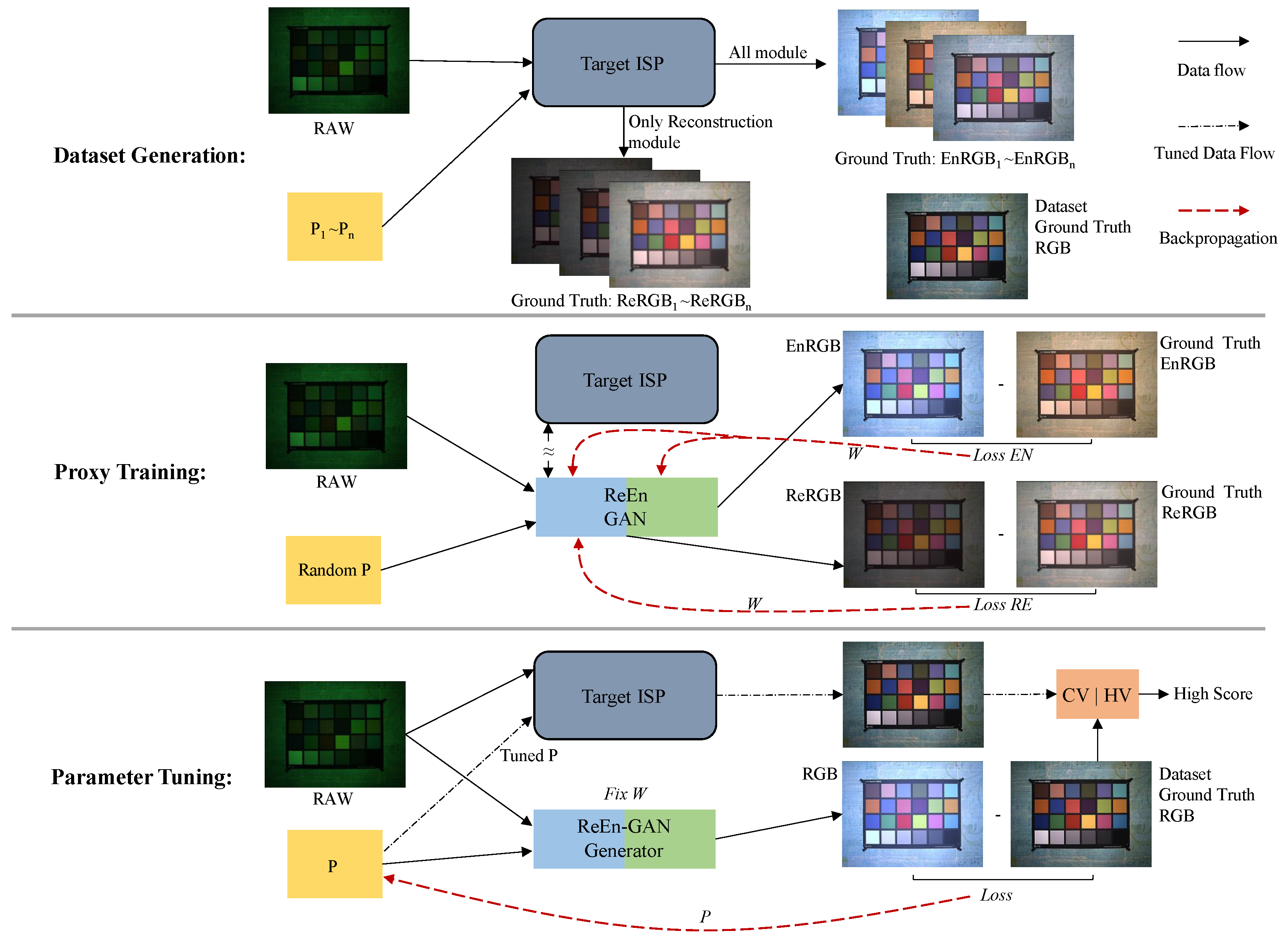
3.1. Overall Proxy Tuning Process

As shown in Figure 1, the tuning method proposed consisted of three steps: step 1, dataset generation; step 2, proxy training; step 3, parameter tuning. In the first step, by injecting randomly selected parameters that cover the parameter space extensively and RAW images into the target ISP, the corresponding ReRGB images and EnRGB images are obtained. Thus, paired RAW-RGB-parameter data are collected. In the second step, by taking paired data as the dataset, the proposed ReEn-GAN is trained separately and jointly to get a two-stage proxy network fitting the target ISP. In the third step, with the ground truth image in the original dataset as the optimization target, parameters with a two-stage proxy are tuned to meet the optimal situation of downstream HV and CV tasks, and the optimal parameters for the target ISP are obtained.
The ultimate goal of ISP tuning is to find the optimal parameters for downstream tasks. For the target ISP pipelines to be tuned, the basic functions are as follows:
f I S P ( I , P ) = f n ( f n 1 ( f 1 ( I , P 1 ) , P n 1 ) , P n )
where f 1 to f n are modules in the ISP pipeline that sequentially process sensor signals, P 1 to P n are parameters for each module, I is the sensor information input to f I S P , and P and I jointly affect the overall output image of f I S P . When I is fixed or follows a certain distribution, adjusting P appropriately can significantly affect the image output by f I S P .
In order to evaluate whether ISP output images can meet certain performance indicators and downstream tasks, an evaluation system is needed as follows:
S = i = 1 N T H V | C V ( f I S P ( I i , P ) ) , I i V
where T H V | C V is the evaluation criterion for f I S P in a certain HV or CV scenario, I belongs to a certain image set or scene V , and S is the score of f I S P in the scene. T H V | C V and V are strictly related; different V requires different T H V | C V as the evaluation function; when V and T are fixed, the only way to improve S is to change P and find the optimal S for T H V | C V under the condition of adjusting P . The optimization function is as follows:
P * = arg min { P } i = 1 N T H V | C V ( f I S P ( I i , P ) ) , I i V
Because the ISP module is in the form of a pipeline, the modules will affect each other. The effect of the latter module f i depends on both its own P i and the processing results of all the previous modules f j | j < i . Therefore, it is difficult to optimize the overall T H V | C V by adjusting the parameters of a single separate module. At the same time, because P in ISP is basically nonlinear and complex, and most of the existing hardware ISP algorithms do not disclose all details to the public, the traditional iterative search method is complex and time-consuming [18]; the complexity of P also determines that it is difficult to use gradient propagation and reverse search methods to search the optimal parameters. Those above problems make the ISP T H V | C V -oriented parameter tuning problem become a nonlinear optimization problem in complex space. When there is a clear evaluation function T H V | C V , some methods refer to the use of a proxy method [13] for HV and CV. The proxy objective is as follows:
W * = arg min { W } i = 1 N f d i f f ( f p r o x y ( I i , P ; W ) , f I S P ( I i , P ) )
where f p r o x y is a differentiable proxy, W is the training parameter of f p r o x y , and f d i f f is a function used to evaluate the magnitude of the difference between the image output by f p r o x y and the image output by f I S P . By adjusting and training W , the sum of f d i f f for I is minimized, and by getting W * , the differentiable proxy of ISP is obtained. Then, by adjusting the input P of f p r o x y , the optimal effect of the proxy under T H V | C V is achieved, and P is given to target f I S P to achieve the optimal effect under T H V | C V . The optimization function is as follows:
P * = arg max { P } i = 1 N T H V | C V f p r o x y I i , P ; W * , I i V
By fixing W * , f p r o x y can adjust the overall image effect on V only by adjusting P , and maximize its score S on HV and CV. Let the P with the largest S be the tuned P * . Then, the best ISP effect on T H V | C V is obtained by reusing P * in f I S P .
As described above, the overall ISP proxy tuning process involves one dataset generation session and two training sessions as shown in Figure 1. The first session, as depicted in Equation (4), involves training the proxy model by minimizing the error between the proxy model output and the actual ISP output. The second session, as depicted in Equation (5), aims to obtain parameters suitable for the actual ISP by maximizing the evaluation score of the proxy model in HV and CV.
Nevertheless, in the proxy training process of [13,20], the parameters within the ISP are treated as equivalent, and the proxy is trained via the same parameter network. This approach results in the end-to-end proxy having to simultaneously learn both low-level (denoising) and high-level (color style) features during the subsequent parameter tuning phase, potentially leading to conflicts in parameter objectives and a decline in proxy performance. Additionally, the employed end-to-end network solely relies on pixel-level loss, thus failing to effectively capture high-frequency details and maintain global consistency in images. As discussed in [14], considering Formula (1), the target ISP pipeline can be divided into two categories: reconstruction and enhancement. For a general ISP pipeline, the processing effect of the two types of modules on images is completely different. Thus, we can split the ISP pipeline into two stages through weak correlation: reconstruction stage and enhancement stage with different optimization goals. Thus, the ReEn-GAN is proposed, which uses a two-stage generative adversarial network as a proxy. By splitting the ISP proxy with all parameters into two different proxies with their own parameters, the above problems can be effectively reduced. The new optimization functions are shown as follows:
W R e * = arg min { W R e } i = 1 N f d i f f [ f R e ( I i , P R e ; W R e ) , f I S P R e ( I i , P R e ) ] , I i V W E n * = arg min { W E n } i = 1 N f d i f f { f E n [ f I S P R e ( I i , P R e ) , P E n ; W E n ] , f I S P ( I i , P ) } , I i V P * = arg max { P } i = 1 N T H V | C V { f E n f R e ( I i , P R e ; W R e * ) , P E n ; W E n * } , ( P E n , P R e ) P
where f R e and f E n are, respectively, the reconstruction proxy and enhancement proxy of the two-stage proxy network. f I S P R e is the target ISP after closing the enhancement modules classified by [14]. In the proxy training step, the training of f R e and the joint training of f R e and f E n are conducted alternately in order to get the best proxy training results. In the parameter tuning step, P * is obtained in the joint training, and loss is passed to P E n and P R e alternately to optimize the global optimal parameters. The overall ReEn-GAN is shown in Figure 2 below.
The goal of reconstruction is to objectively reconstruct the physical scene, which requires strict adherence to sensor physical constraints (such as Bayer array interpolation kernel, noise model), and optimization metrics mainly include PSNR and SSIM. The goal of enhancement is to improve subjective visual quality, which needs to meet human perceptual preferences, and optimize indicators mainly based on perceptual similarity. In the ISP pipeline, the modules classified as reconstruction include demosaic, denoise, edge enhancement, etc.; the modules classified as enhancement include white balance, color correction, etc. In the ISP pipeline, modules classified as reconstruction and enhancement have vastly different effects on image processing [14]. Therefore, for Re-stage and En-stage proxies, specific network structures and loss functions can be used to optimize different proxy targets in these two scenarios; specific training and tuning scheme are needed for more effective optimization; and a specific training environment and experimental scenarios are required to achieve more efficient proxy training. Therefore, it is necessary to point out the specific optimization content in the network structure, loss function, training tuning scheme, and experiment sections. The rest of this section will discuss the ReEn-GAN, its loss functions, training, and tuning scheme in detail, and the experiment environment will be discussed in the Section 4.

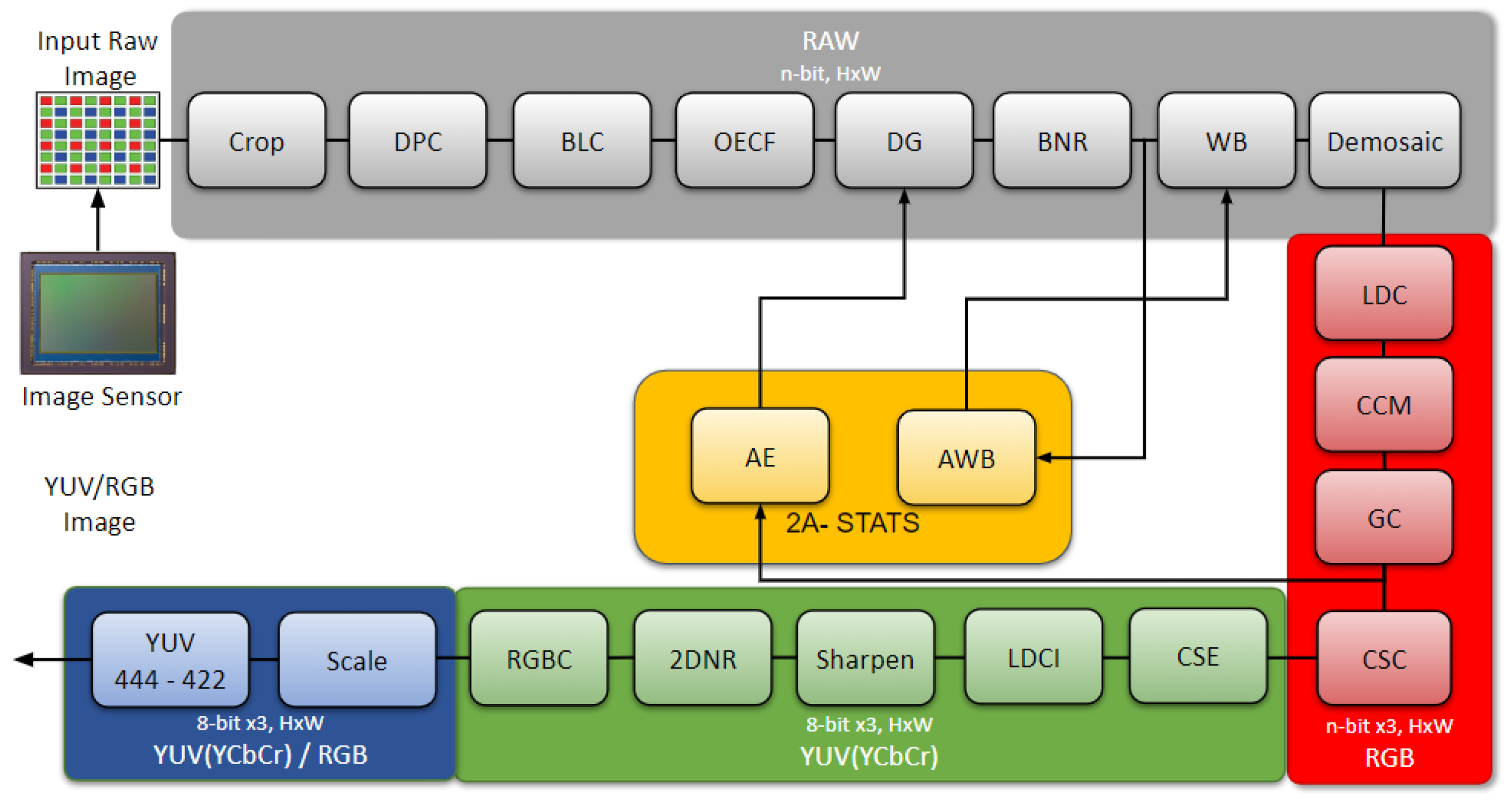
3.2. Reconstruction Stage

In the ISP pipeline, the primary objective of the reconstruction phase is to transform sensor RAW data into high-quality linear RGB images while preserving the original details within the images. For the scenario of ISP reconstruction, in order to optimize the proxy network more effectively and make it suitable for Re-stage scenarios, a specific network structure needs to be used. There are many network structures to choose from, and for image-to-image tasks, we first consider the U-net model [33] as the network structureused for image segmentation tasks. Due to its encoder–decoder structure, the information at all levels of the image can be transmitted across layers through skip connections, making it suitable for image transfer tasks that preserve image details. Meanwhile, in image reconstruction task scenarios, the corresponding ISP module is mainly used for image restoration tasks such as noise reduction, sharpening, and demosaicing, with higher requirements for image details. Therefore, U-NET is often used as the network structure in many AI–ISP applications [23]. At the same time, as a RAW-to-RGB transfer task, image reconstruction requires the network to be able to specifically adapt to the input of RAW images and the output of RGB images, as well as to preserve the structure and information of the input image well. Therefore, based on the four-layer U-Net, we changed the input structure of the network to accept RAW input and ISP parameter input to preserve the original information of the image while the network has sufficient scalability to obtain information on the influence of different ISP parameters on the image. For the discriminator, in order to obtain detailed information of the image, we use patch discriminator to obtain the L G A N , which allows D1 to better control the image generated by G1 through patch level of loss. Generally speaking, the generator employs an optimized encoder–decoder architecture akin to U-Net, while the discriminator utilizes patch discriminators and loss functions described in Equation (7), as depicted in Figure 3.
During the reconstruction phase, generator G 1 is required to capture the spatial transformation features of the image from RAW to RGB in the ISP pipeline, while also implementing image detail processing such as denoising and sharpening. The basic structure of G 1 is an encoder–decoder U-Net with four layers of skip connections. In order to reduce the problems of image artifacts and edge blur caused by the direct input of Bayer images into the network [32], pixel shuffle [34] is applied before the input layer of the network. By rearranging the pixels of the Bayer array, the raw image in the shape of H × W × 1 is replaced with H / 2 × W / 2 × 4 { R , G , B , G } images, which reduces the size of the RAW image and decreases the computational complexity of the network, while avoiding the edge blur and mosaic problems caused by the direct processing of Bayer images [35]. The input image in the shape of H / 2 × W / 2 × 4 undergoes one flat convolution and four down-flat convolutions to encode the image. In order to enable the network to better learn the impact of P R e on the image effect, the image will be concatenated with the corresponding size parameter matrix before each convolution layer, so that all information of P R e can be captured in each convolution. The output data size of the encoder is H / 32 × W / 32 × 256 , and the data enters the decoding stage to restore the details of the image at all levels and achieve the overall reconstruction of the image. At the same time, the concatenated data is linked to the decoder through a skip connection [33], which directly transfers low-level features (such as edges, textures, etc.) to high-level feature maps, helping the network preserve detailed information during the reconstruction process and reducing the problem of vanishing gradients, thereby accelerating the training process and improving reconstruction quality. After going through the encoder–decoder network, the input data in the shape of H / 2 × W / 2 × 4 is converted into the output data in the shape of H / 2 × W / 2 × 12 , which are four channels of R, four channels of G, and four channels of B, respectively. After pixel reshuffle [36], the final output of H × W × 3 is the { R , G , B } image data. In D 1 , in order to enable the discriminator to better obtain hierarchical perceptual information of the image, patch-GAN is used as the discriminators to capture information at various levels.

3.3. Enhancement Stage

In the enhancement stage, the training target of the proxy is the module used for image enhancement in ISP. The proxy takes plain { R , G , B } as the image input, learns the enhancement module to perform color correction, white balance correction, and other effects on the image to obtain the proxy, and outputs the enhanced { R , G , B } image. Similar to the reconstruction stage, in the proxy training of the reconstruction stage, the main goal of the network is also the conversion task of image-to-image. Therefore, U-Net is also used as the basic network structure, and the encoder–decoder structure and skip connection are used to achieve the synthesis and restoration of information at various levels of the image while preserving a certain amount of network learning space for learning the impact of ISP parameter changes on the image. Unlike Re-stage, En-stage serves as a fitting for ISP image reconstruction step, mainly fitting modules such as color correction and white balance in ISP. Therefore, it has lower modeling requirements for image details and higher fitting requirements for overall chromaticity and contrast. Therefore, a network of En-stage can be designed to more efficiently learn the impact of ISP parameters on image effects based on the above characteristics. We use a three-layer U-Net as the network backbone. Compared to the four-layer U-Net used in restoration, we reduce the number of layers to reduce the overall feature extraction scale of the network while retaining a certain feature extraction ability. At the same time, we use a PPM [37] module to enable the network to capture global information at various levels of the image, which corresponds to the color and texture information of the image. Meanwhile, due to the En-stage processing image pairs of RGB-to-RGB, a normal image input layer is used. For the discriminator, in order to obtain the overall information of the image, we use global discriminator to obtain the L G A N , which allows D2 to better control the image generated by G2 through global level of loss. Generally speaking, the enhancement stage uses an encoder–decoder structure similar to U-Net with pyramid pooling module(PPM) [37] as Generator, and evaluates the output images at global levels using global discriminators and loss functions described in Equation (8). The structure of the enhancement stage is shown in Figure 4.
The enhancement stage mainly requires G2 to capture color restoration or tone information in ISP, so the restoration of details at various levels of the image does not need to be like G1, but only needs to focus on the color information of the image and the style information of each level of the image. Therefore, the structure of G2 is similar to G1, using a skip connection encoder–decoder structure similar to U-Net, reducing one layer of encoding and decoding hierarchy and adding a pyramid pooling module(PPM) [37] to enhance the decoder’s multi-scale context awareness ability, achieving better color restoration effect. The input of G2 is a reconstructed three-channel RGB image in size of H × W × 2 . After one flat convolution and three down-flat convolutions, the encoded information in size of H / 8 × W / 8 × 64 is obtained. After being encoded by the encoder, the data enters the PPM module and is up-sampled through four different-sized max pooling layers of ( [ 2 , 2 ] , [ 4 , 4 ] , [ 16 , 16 ] , [ 32 , 32 ] ) to capture the image information of each level. It is then concatenated with the original encoded information and sent to the decoder. In the decoding section, the output image EnRGB in the shape of H × W × 3 is obtained through three layers of up convolutions and one layer of flat convolution. In D 2 , in order to enable the discriminator to better obtain global perceptual information of the image for color reproduction, global-GAN is used as the discriminators to capture global color information.

3.4. Loss Function

The two stages of ReEn-GAN use different loss functions respectively, in order to obtain different optimization objectives and losses of images in the two stages.
In the reconstruction stage, in order to capture the detail of the image, as well as to make G R e faithfully reconstruct the scene—which contains genuine image structures from RAW image data—and the effect of P R e on images, specific loss functions are required. In ISP restoration, it is necessary for the network to learn the detailed reconstruction features of the image. Therefore, based on L G A N , the addition of L 1 can enable the network to learn the detailed features of the image without causing blurring like L 2 . Meanwhile, by incorporating the perceptual loss of pre-trained network loss L V G G , the generated images of the network can be perceived similarly rather than at the pixel-level. Therefore, the mutual compensation between L 1 and L V G G can enhance the learning ability of the network. As mentioned earlier, the use of L p a t c h G A N can also improve the network’s perception of details and enhance its overall generalization ability. Therefore, we use the combination of L 1 , L p a t c h G A N , and L V G G as the loss function in the reconstruction stage. The loss functions are shown as follows:
L R e = L p a t c h G A N + α 1 L 1 + α 2 L V G G L p a t c h G A N ( G R e , D R e ) = E I , I G T [ log D ( I , I G T ) ] + E I ( log { 1 D [ I , G ( I ) ] } ) L 1 = E I , I G T [ | | I I G T | | 1 ] L V G G ( I , I G T ) = min G R e i = 1 5 1 C i W i H i B i ( I ) B i ( I G T ) 2 2
where α 1 and α 2 control the importance of L 1 and L V G G . C i , W i and H i indicate the channels, width, and height of the corresponding output feature map, respectively. Using L 1 instead of L 2 is to avoid the blur effect. L V G G is based on a pre-trained VGGNet [38].
In the enhancement stage, in order to capture the color and global perceptual distribution of the image, as well as to make G E n faithfully reconstruct the scene—which contains genuine image color from RGB image data—and the effect of P E n on images, specific loss functions are also required. In the enhancement stage of ISP, it is necessary for the network to learn the overall information of the image, while also preserving some details of the image so that the proxy can more effectively control the influence of ISP parameters on the image. Therefore, on the basis of L G A N , adding L 1 enables the proxy to learn the pixel-level information of the image more effectively, and by adding L c o l o r [39], the network can learn macro color information. Through L c o l o r , the proxy can learn the influence of parameters on the chromaticity of the image more effectively. By integrating L g l o b a l G A N and L c o l o r , as well as complementing L 1 , the network can be trained more effectively and enhance overall generalization. Therefore, we use the combination of L 1 , L g l o b a l G A N , and L c o l o r as loss function in the enhancement stage. The loss functions are shown as follows:
L E n = L g l o b a l G A N + β 1 L 1 + β 2 L c o l o r L g l o b a l G A N ( G E n , D E n ) = E I , I G T [ log D ( I , I G T ) ] + E I ( log { 1 D [ I , G ( I ) ] } ) L 1 = E I , I G T [ | | I , I G T | | 1 ] L c o l o r ( I , I G T ) = | | I b I G T b | | 2 2
where β 1 and β 2 control the importance of L 1 and L c o l o r . As we did before, we use L 1 to avoid blur effect by G E n . I b and I G T b are images blurred by a 2D Gaussian blur operator, which are used for color loss [39].

3.5. Proxy Training and Tuning Scheme

In this section, we will briefly discuss the proxy training and tuning scheme. As mentioned above, the two-stage proxy training uses the method of staged and joint training. Due to the difference between the reconstruction stage and the enhancement stage in the ISP pipeline, the two stages of proxy training use different learning rate (LR), number of epochs, size of batch, etc. The specific training environment will be discussed in the Section 4. Firstly, the two networks of the reconstruction stage and the enhancement stage need to be trained separately. For the Re-stage, the loss function is L R e , as mentioned above. I R e is obtained by turning off the En module of target ISP, and I R A W and I R e as I G T are used as the input and output of the network. D R e is used to provide L p a t c h G A N , while the output of G R e is used to calculate L 1 and L V G G . At the same time, the En-stage also needs to conduct training synchronously, using L E n as the loss function, obtaining I E n through the complete target ISP, using I R e and I E n as the input and output of the network, and using D E n for the L g l o b a l G A N , and the output of G E n as I G T is used to calculate L 1 and L c o l o r .
When the training of G R e and G E n converges, the joint fine-tuning of G R e and G E n will be conducted. We use I R A W , I R e and I E n as the input and I G T of the two-stage proxy, respectively, obtain a joint two-stage proxy through alternate training, and use the equal combination of L R e and L E n without L G A N as the loss function. G E n accepts the gradient from the L R e part, while G R e accepts the gradient from the complete combined loss function [14].
In the tuning stage, the training parameters of the trained two-stage proxy will be fixed, and L 1 is used as the loss function, which will be back-propagated to the ISP parameters of the proxy. The tuning details can be seen in the Section 4.4 and Section 4.5 below.

4. Experiments

4.1. Experimental Environment and Dataset

The experiments in this paper were conducted using an Intel Xeon Platinum 8255C CPU and an NVIDIA RTX 4080 GPU with CUDA version 11.7. To verify the performance of this method on CV tasks, we selected denoising and object detection as downstream tasks. We used the open-source Infinite-ISP [40] as the tuning target and validated the effectiveness of denoising and object detection using the SIDD [41] and KITTI datasets [42,43], respectively.

4.2. Data Generation and ISP Tuning Preparation

This article uses the open-source InfiniteISP [40] as a software ISP for tuning, and its pipeline is shown in Figure 5 below:
Infinite-ISP includes common algorithms in the ISP pipeline, and it also exposes many parameters that can be tuned externally. This paper selects seven modules, BLC (black level correction), BNR (Bayer noise reduction), AWB (auto white balance), CSE (color saturation enhancement), sharpen, LDCI (local dynamic contrast improvement), and 2DNR (2D noise reduction) as the target modules for tuning, while the parameters of the remaining modules are fixed as default. According to the classification rules in [14], the seven modules are divided into two categories: reconstruction and enhancement, where BLC, BNR, sharpen, and 2DNR are tuning targets for the reconstruction stage, while AWB, CSE, and LDCI are tuning targets for the enhancement stage. All tuning parameters are shown in Table 1 below:
The above parameters are randomly generated within the range and sent to Infinite-ISP to obtain the target ISP for each parameter combination. The intermediate values for reconstruction and enhancement of the two training sessions need to be obtained by turning off AWB, CSE, and LDCI.
For the denoising tuning dataset, we used the SIDD Medium RAW dataset and selected a total of twenty-eight images with different exposures from seven different scenes as the original images. We randomly generated a parameter set of eighteen parameters for tuning and combined it with twenty-eight images to form a dataset of 2800 image-parameter pairs as the first step for training the proxy.
For the object detection tuning dataset, we use the KITTI dataset to select the object detection scene for generating the raw images for training the proxy. At the same time, in order to verify the performance of the tuning effect in object detection in this article, Fast R-CNN [44] was used to train a network for object detection on KITTI, and it was applied to the proxy loss calculation of CV tasks.

4.3. Proxy Performance Experiment

In this section, in order to verify the advantages of the proposed two-stage proxy compared with the end-to-end proxy in terms of image quality, a comparison was made between the two methods for generating proxy images under certain convergence conditions, as well as the quality of the generated images under parameter changes. By comparing the proxy output and ISP output under random parameters in SSIM and HC mentioned above, the difference is evaluated. In order to verify structural similarity more specifically, the SSIM are optimized to be more focused on structure difference [31]. The optimized SSIM functions and HC functions are shown as follows:
S S I M ( I p r o x y , I I S P ) = [ l ( I p r o x y , I I S P ) 0.2 · c ( I p r o x y , I I S P ) 2.8 · s ( I p r o x y , I I S P ) 3.5 ]
H C I 1 , I 2 = i = 1 N H 1 ( i ) H ¯ 1 H 2 ( i ) H ¯ 2 i = 1 N H 1 ( i ) H ¯ 1 2 · i = 1 N H 2 ( i ) H ¯ 2 2
Considering Equation (9), l, c, and s are metrics for luminance, contrast, and structure, respectively [27]. By adjusting the weight of those metrics [31], SSIM can measure structural differences more specifically, while assigning the task of distinguishing color differences to HC. Considering Equation (10), H 1 and H 2 are the histograms of two pictures, respectively, while H ¯ 1 and H ¯ 2 are mean of histogram. The Pearson Correlation Coefficient between the histograms of two images is calculated to get the value that measures the correlation between the chromaticity statistics of two images. Along with the measurement of the above two metrics, we also calculated the number of trainable parameters and forward propagation FLOPs of those two proxy networks.
In the process of proxy training, as mentioned above, different LR and patch sizes are used. In the process of Re-stage training, we use ADAM ( β 1 = 0.9, β 2 = 0.99) as the optimizer. The LR of G R e and D R e are set to 0.0002 and 0.00005, respectively. We use a batch size of 12. After about epoch 300, G R e gradually converges. Among them, α 1 and α 2 in L R e have undergone our limited tests. At the same scale, changes in value have little impact on G R e reception, and we set them to 0.01 and 1. At the same time, En-stage also needs to be trained. The same ADAM ( β 1 = 0.9, β 2 = 0.99) is used as the optimizer. The LR of G E n and D E n are set to 0.001 and 0.0005, respectively, due to the En-stage being easier to converge than the Re-stage, and the network is also smaller. Similarly, a batch size of 12 is used. After about 200 epochs, G E n gradually converges. The β 1 and β 2 of L E n have undergone our limited tests. Similar to the Re-stage, the same scale has less impact on G E n convergence, so it is set to 0.01 and 10. After the convergence of the rest and En-stage training, the joint training is carried out. In the joint training, the loss function is the equal combined loss function mentioned above. Similarly, the ADAM optimizer ( β 1 = 0.9, β 2 = 0.99) is used, and LR is set to 0.0005, and a batch size of 8 is used. After training of approximately epoch 150, the convergence trend begins to end. After proxy training, optimized SSIM and HC are used to evaluate the proxy performance of two-stage proxy and end-to-end proxy [20]. The results are shown in Table 2.
From this table, we can see that, compared to optimized SSIM, the proposed method has a greater improvement on HC. Due to the fact that HC measures more the differences in color and brightness, while optimized SSIM focuses more on the differences in structure and details, the two-stage proxy method proposed is more effective in restoring color and brightness compared to the end-to-end proxy method. This confirms the significance of splitting the ISP pipeline into reconstruction and enhancement, which utilizes different loss functions and optimization objectives in the reconstruction and enhancement stages to achieve the separation of detail processing and color processing, thereby improving the proxy’s ability to grasp information from various dimensions of the image. Better proxy effects also lead to amplifying the improvement of the tuning performance for downstream tasks shown later in this section.
We can also see that, compared with the end-to-end proxy method, the proposed two-stage proxy method uses significantly more network parameters and computation cost, almost a doubling of Params and FLOPs due to the fact that the two-stage proxy method decouples the ISP into two proxies that need to train separately. The need for more computation cost also leads to a longer time consumption of the optimal parameter search process in the tuning phase shown later in this section.

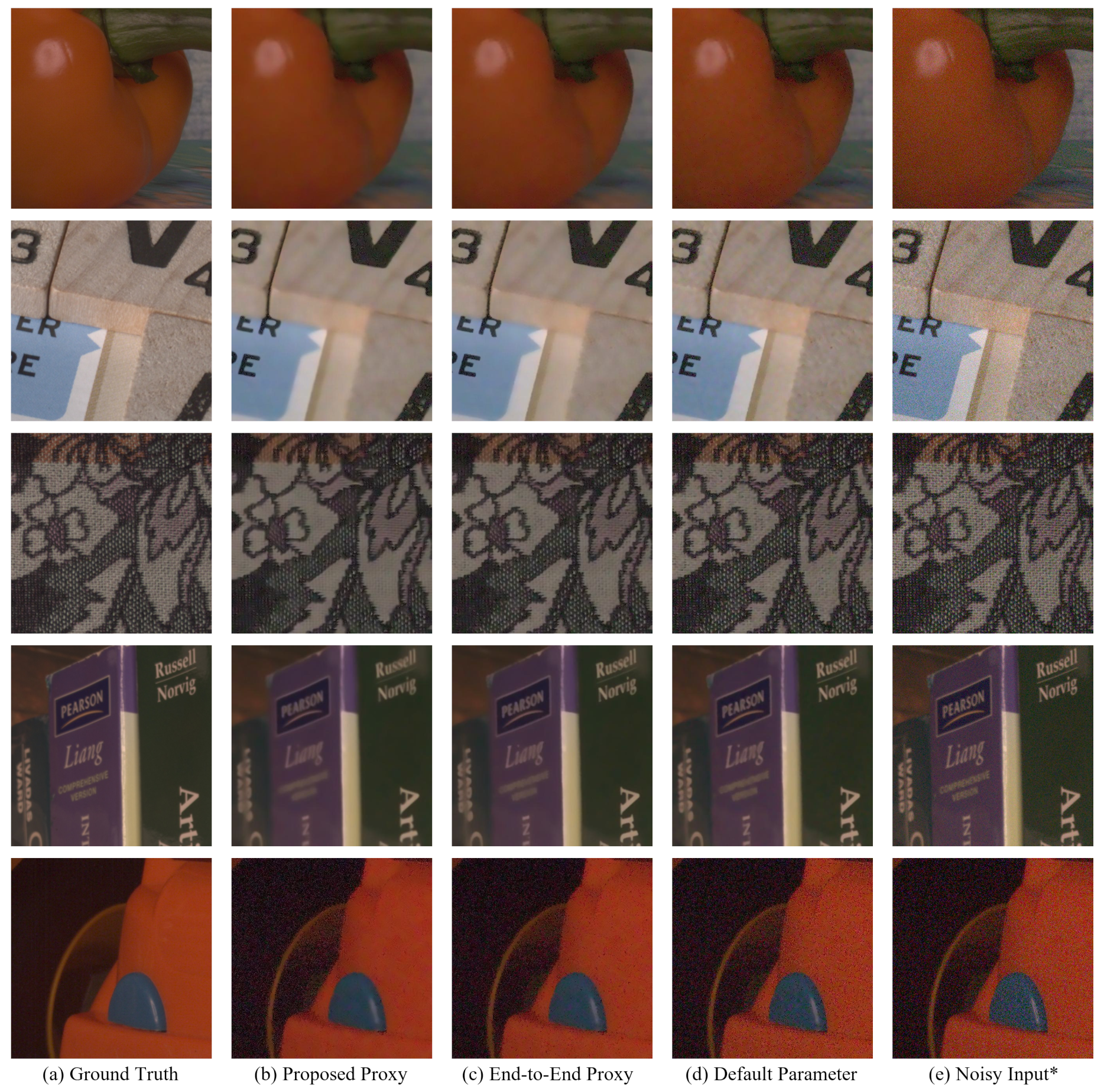
4.4. Denoising Tuning Experiment

In this section, to verify the effectiveness of the ReEn-GAN method proposed in this paper compared to end-to-end proxy, hand-tuning, and other methods, we compared the ISP parameters generated by each method on the image denoising task after applying them to Infinite-ISP. In addition to the parameter generation methods mentioned above, we also compared the results of default parameters, random parameters, and extra BM3D to demonstrate the effectiveness of the tuning method. The criteria we used in our evaluation are PNSR and SSIM, by calculating the PSNR and SSIM between ground truth images and ISP processed images with parameters obtained by various methods to obtain the effects of different tuning methods and facilitate quantitative comparison. The equation of PSNR and SSIM are shown as follows:
P S N R ( x , y ) = 10 · log 10 MAX 2 MSE ( x , y ) M S E ( x , y ) = 1 M · N i = 0 M 1 j = 0 N 1 [ x ( i , j ) y ( i , j ) ] 2 S S I M ( x , y ) = 2 μ x μ y + C 1 2 σ x y + C 2 μ x 2 + μ y 2 + C 1 σ x 2 + σ y 2 + C 2
where MAX is the maximum value of pixels in the image, M and N are the length and width of the image, respectively, C 1 and C 2 are constants often set as ( 0.01 M A X ) 2 and ( 0.03 M A X ) 2 , and the MSE is Mean Square Error.
In the denoising tuning step, we randomly initialize the hyper-parameters P . As mentioned above, we use L 1 as loss function. We use ADAM optimizer ( β 1 = 0.9, β 2 = 0.999) and a LR of 0.000005. After about epoch 20, the P tend to convergent. Then, the P are used in the Infinite-ISP to get the output images alone with PSNR and SSIM in average. The results are shown in Table 3 below.
From this table, we can see that firstly, compared to random parameters, the noise reduction effect of ISP with default parameters or adjusted parameters is greatly improved, indicating that the adjustment of parameters has a particularly important impact on the quality of ISP image processing. Secondly, compared to the ISP with default parameters, the ISP with hand-tuned parameters has a greater enhancement effect on SSIM than on PSNR, indicating that hand-tuning pays more attention to the structural loss of images than to noise. Hand-tuning is more suitable for modules that have a significant impact on human perception and is not widely applicable to any downstream task. Thirdly, the effect of using the proxy method for tuning is better than hand-tuning, indicating that for general downstream tasks, using the proxy method can significantly improve the effect, and there is also an improvement in timeliness compared to time-consuming manual tuning. Last but not least, compared with the tuning method using end-to-end proxy, the performance improvement of the proxy method proposed in this paper on the SSIM index is greater than that on PSNR, indicating that the scheme of using staged reconstruction to enhance the proxy can eliminate the perceptual changes in the image caused by the enhancement stage in the reconstruction proxy stage compared to the end-to-end proxy scheme of a single network. At the same time, using generative adversarial networks can also make the generalization ability of the generative network stronger, making the proxy better able to represent the structural information of the image, resulting in a greater improvement in the SSIM index compared to PSNR. Part of the test result is shown in Figure 6.

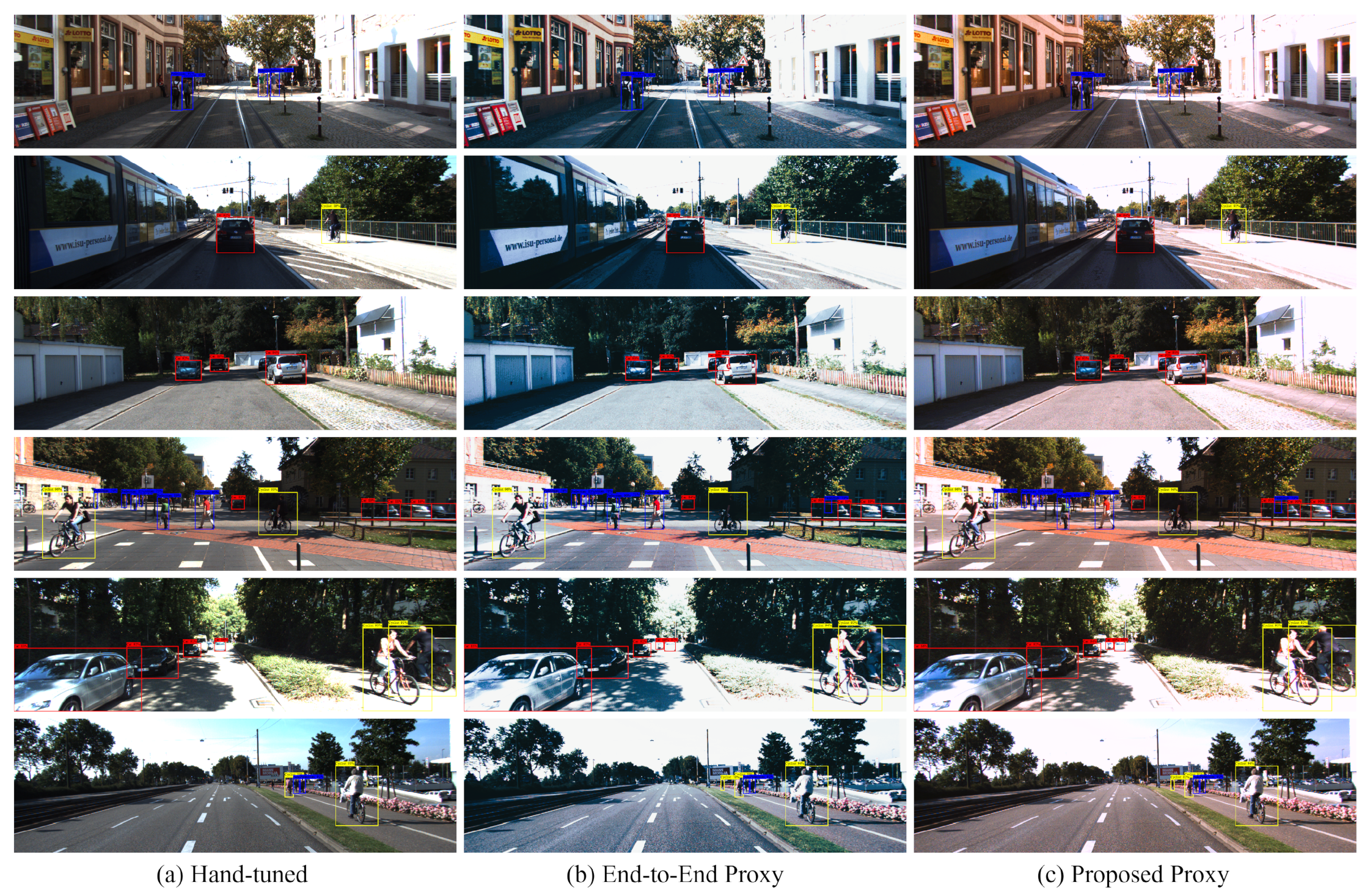
4.5. Object Detection Tuning Experiment

This section evaluates the effectiveness of various parameter generation methods on Infinite-ISP using object detection tasks and assesses the image object detection performance using Fast R-CNN trained on KITTI. The training of Fast R-CNN is based on the KITTI dataset, and the labels in the KITTI dataset are merged into three major categories, namely car, pedestrian, and cyclist.
In this section, similar to the previous section, the proposed proxy method will be compared with end-to-end proxy, hand-tuning, random parameters, and default parameters to compare the performance of the parameters generated by the above methods on object detection tasks in Infinite-ISP. The criteria we used to evaluation are Average Precision (AP), True Positive (TP), False Negative (FN) and F1 score, where AP@0.5/% are used to evaluate the object detection performance of each method on three types of targets (car, person, bicycle). The mAP@0.5/% averages the object detection performance of the three types of targets to get the overall object detection performance. TP and FN are used to count correctly detected targets and incorrectly detected targets, respectively, where TP counts the number of prediction boxes with Intersection Over Unions (IOUs) greater than the threshold (properly predicted), and FN counts targets not properly predicted. The F1 score is used to evaluate the balance performance of Precision and Recall; the calculation formulas are shown as follows:
P r e c i s i o n = T P T P + F P R e c a l l = T P T P + F N F 1 = 2 · P r e c i s i o n · R e c a l l P r e c i s i o n + R e c a l l
where False Positive (FP) is the number of prediction boxes with IOUs less than the threshold.
In the object detection tuning step, we randomly initialize the hyper-parameters P . As mentioned above, we use L 1 as loss function. We use ADAM optimizer ( β 1 = 0.9, β 2 = 0.999) and an LR of 0.000005. After about epoch 35, the P tend to convergent. Then, the P are used in the Infinite-ISP to get the output images. By calculating all the above-mentioned metrics on object detection task with the ISP-processed images with parameters obtained by various methods, the effects of different tuning methods are obtained to facilitate quantitative comparison. The results are shown in Table 4 below:
From this table, we can see that firstly, compared to the improvement in tuning effect for denoising tasks, the improvement in tuning effect for object detection is smaller, indicating that CV tasks such as object recognition are less sensitive to ISP parameter adjustments. At the same time, compared to default parameters, the performance degradation of random parameters in object recognition tasks is smaller than that in denoising tasks, which also indicates that the necessity of parameter adjustment varies in various tasks. Secondly, we can see that in the process of using proxy tuning instead of hand-tuning, compared to the performance improvement of denoising tasks on SSIM, the performance improvement of object detection tasks is more significant, while compared to denoising tasks, the performance improvement on PSNR is even less significant. This indicates that the use of the proxy tuning method has a tendency to improve the performance of different tasks, which also confirms the previous conclusion. Furthermore, similar to denoising tasks, there is a clear upper limit to the performance improvement of hand-tuning, and using proxy tuning can break through this upper limit in certain indicators. Although the overall performance improvement is not as good as denoising tasks, the application of proxy tuning in object detection can effectively break through the upper limit of hand-tuning. This means that the proxy model can find the global optimal solution by searching for various specific optimal solutions for CV tasks and get rid of the performance degradation of CV tasks caused by human eyes’ specific understanding and preferences for images (as shown in Figure 7, poor visual perception does not necessarily mean poor CV performance). Last but not least, the method proposed in this article further improves the performance of object detection tasks on the basis of end-to-end proxy, demonstrating that by decoupling the reconstruction enhancement task and adding L G A N , the two-layer proxy can capture more features of the ISP pipeline’s impact on the image, allowing the proxy to better fit the ISP pipeline under different parameter conditions, thereby achieving better tuning performance in downstream CV tasks. Part of the test result is shown in Figure 7.

4.6. Ablation Experiment

In this section, we will compare the significance of different loss functions and PPM in the proposed methods. In order to demonstrate the effectiveness of the proposed method, we compared the performance differences of the model in proxy fitting performance and denoising tuning performance under different conditions. The results are shown in Table 5 below. The metrics and experiment settings are mentioned earlier.
From the proxy fitting part of this table, we can see that compared to PPM, the performance improvement of L V G G and L c o l o r is more significant, with the addition of L V G G leading to a more significant improvement in proxy SSIM of proxy fitting results, while the addition of L c o l o r leads to a more significant improvement in proxy HC. However, the difference in performance improvement between PSNR and SSIM in tuning experiments is not significant. Meanwhile, since the main improvement of the proposed method lies in the improvement of two-stage compared to end-to-end, the impact of the loss function and PPM on overall performance is relatively small. The experiment on the difference between the proposed two-stage proxy and end-to-end proxy has been discussed in the proxy performance experiment above.

5. Discussion

In the methods and experimental results above, we compared the performance of the proposed two-stage proxy and end-to-end proxy methods in various dimensions. Firstly, we compared the differences in proxy performance between two methods. By comparing specific optimized SSIM and HC, we validated the proxy effect of the proposed method on image structure and color, demonstrating that it can better grasp the chromaticity information of images compared to the end-to-end proxy method. Secondly, we compared the tuning effects of two proxy methods and a manual tuning method on downstream tasks such as object detection and noise reduction, and used the evaluation indicators of each task to indicate the tuning effect. The results showed that the proposed proxy method had certain improvements in both object detection and noise reduction tasks compared to the end-to-end proxy method and the manual tuning method. Moreover, due to the more obvious restoration effect of the proposed method on ISP color processing compared to structural restoration, the improvement of the proposed method on object detection tasks compared to end-to-end proxy was greater than that on noise reduction tasks. Meanwhile, the proxy based tuning method significantly improves the tuning effect for CV tasks compared to manual tuning, demonstrating the superiority of the proxy tuning method in CV tasks. Thirdly, we compared the effects of different loss functions and PPM on the proposed two-stage proxy. The experiment showed that by setting a reasonable loss function and adding a PPM module, the proxy performance and downstream tuning performance of the staged proxy can be effectively improved, and the performance can be further improved on the basis of the staged improvement.
We can also see that the proposed two-stage proxy method has some room for improvement. In the above experimental results, it is shown, firstly, that compared to the end-to-end proxy method, the proposed two-stage method has significant disadvantages in terms of computational complexity for proxy fitting. This is reflected in the fact that the two-stage proxy needs to learn the reconstruction and enhancement proxy of ISP pipelines separately, and the complexity of the corresponding tuning steps will also increase. Meanwhile, due to the addition of various loss functions, the convergence speed of the proxy has also been reduced, resulting in a decrease in the timeliness of the proposed method compared to the end-to-end method. Secondly, compared to the end-to-end method, the proposed two-stage method does not strictly belong to the black-box method because it utilizes the internal information of the ISP pipeline. When encountering an ISP that is completely black-box to the outside tuner, the two-stage proxy method may have a reduced fitting effect on the ISP pipeline due to the inability to obtain information between ISP modules, resulting in a decrease in tuning performance. Thirdly, due to the limitation of experimental time, this article did not extensively experiment with the improvement of two-stage proxy performance by various loss functions, the tuning performance of more different ISPs, and the tuning effect of more downstream CV tasks.
Therefore, based on those above issues, there is still a lot of future research space on the basis of this paper. Firstly, on the basis of the existing network structure, the network structure of the reconstruction and enhancement stages can be improved to achieve similar proxy performance at lower complexity. Secondly, by improving the structure of how the parameters are inputted to the network, on the basis of the existing two-stage proxy method, different types of parameters can also correspond to different types of network structures, thereby further enhancing the proxy performance of the model on different category ISP modules. Thirdly, testing of the impact of changing more loss functions and different feature extraction modules on the proxy and tuning performance of the model can be done in order to optimize proxy performance and tuning performance more thoroughly.

6. Conclusions

This paper proposes an ISP tuning method based on two-stage proxy. By decoupling the ISP process into a reconstruction phase (physical signal recovery) and an enhancement phase (visual quality and color optimization), the two-stage proxy can better fit different modules in ISP. By using different network structures and loss functions for different targets, the two-stage proxy can efficiently fit the reconstruction and enhancement modules in ISP. In the Section 4, firstly, this article compared the performance differences between the two-stage proxy and end-to-end proxy in terms of proxy performance and downstream CV tuning tasks and demonstrated the importance of the two-stage proxy. Secondly, by comparing the performance differences of different tuning methods on the downstream CV tasks of denoising and object detection, the performance improvement of proxy tuning compared to manual tuning and the performance improvement of the two-stage proxy tuning method compared to the end-to-end proxy tuning method were verified. Thirdly, by comparing different loss functions, the significance of improving the loss function for performance enhancement in addition to the two-stage proxy was verified in this paper. Those experiments have shown that this method outperforms traditional ISP and end-to-end proxy methods on public datasets (SIDD, KITTI) and outperforms hand-tuning by more than 21% in performance metrics.

Author Contributions

Conceptualization, J.Y. and P.Z.; methodology, P.Z.; software, P.Z.; validation, P.Z.; investigation, P.Z.; writing—review and editing, P.Z. and J.Y.; supervision, J.Y. All authors have read and agreed to the published version of the manuscript.

Funding

This research received no external funding.

Institutional Review Board Statement

Not applicable.

Informed Consent Statement

Not applicable.

Data Availability Statement

The original contributions presented in this study are included in the article. Further inquiries can be directed to the corresponding author.

Conflicts of Interest

The authors declare no conflicts of interest.

Abbreviations

The following abbreviations are used in this manuscript:
ISPImage Signal Processor
CVComputer Vision
HVHuman Vision
PPMPyramid Pooling Module
BLCBlack Level Correction
BNRBayer Noise Reduction
AWBAuto White Balance
CSEColor Saturation Enhancement
LDCILocal Dynamic Contrast Improvement
2DNRTwo-dimensional Noise Reduction

References

  1. Brown, M.S. Understanding the In-Camera Image Processing Pipeline for Computer Vision. In Proceedings of the IEEE Computer Vision and Pattern Recognition-Tutorial, Las Vegas, NV, USA, 26 June–1 July 2016. [Google Scholar]
  2. Guo, Y.; Wu, X.; Luo, F. Learning Degradation-Independent Representations for Camera ISP Pipelines. In Proceedings of the 2024 IEEE/CVF Conference on Computer Vision and Pattern Recognition (CVPR), Seattle, WA, USA, 16–22 June 2023; pp. 25774–25783. [Google Scholar]
  3. Wu, C.T.; Isikdogan, L.F.; Rao, S.; Nayak, B.; Gerasimow, T.; Sutic, A.; Ain-kedem, L.; Michael, G. VisionISP: Repurposing the Image Signal Processor for Computer Vision Applications. In Proceedings of the 2019 IEEE International Conference on Image Processing (ICIP), Taipei, Taiwan, 22–25 September 2019; pp. 4624–4628. [Google Scholar] [CrossRef]
  4. Yang, C.; Kim, J.; Lee, J.; Kim, Y.; Kim, S.S.; Kim, T.; Yim, J. Effective ISP Tuning Framework Based on User Preference Feedback. Electron. Imaging 2020, 32, 1–5. [Google Scholar] [CrossRef]
  5. IEEE Std 1858-2016; IEEE Standard for Camera Phone Image Quality. IEEE: New York, NY, USA, 2017; pp. 1–146. [CrossRef]
  6. IEEE P2020 Automotive Imaging. 2018, pp. 1–32. Available online: https://ieeexplore.ieee.org/document/8439102 (accessed on 13 November 2024).
  7. Microsoft. Microsoft Teams Video Capture Specification, 4th ed.; Microsoft: Redmond, WA, USA, 2019. [Google Scholar]
  8. Wueller, D.; Kejser, U.B. Standardization of Image Quality Analysis–ISO 19264; Society for Imaging Science and Technology: Scottsdale, AZ, USA, 2016. [Google Scholar]
  9. Yahiaoui, L.; Horgan, J.; Deegan, B.; Yogamani, S.; Hughes, C.; Denny, P. Overview and Empirical Analysis of ISP Parameter Tuning for Visual Perception in Autonomous Driving. J. Imaging 2019, 5, 78. [Google Scholar] [CrossRef] [PubMed]
  10. Molloy, D.; Deegan, B.; Mullins, D.; Ward, E.; Horgan, J.; Eising, C.; Denny, P.; Jones, E.; Glavin, M. Impact of ISP Tuning on Object Detection. J. Imaging 2023, 9, 260. [Google Scholar] [CrossRef] [PubMed]
  11. Yoshimura, M.; Otsuka, J.; Irie, A.; Ohashi, T. DynamicISP: Dynamically Controlled Image Signal Processor for Image Recognition. In Proceedings of the 2023 IEEE/CVF International Conference on Computer Vision (ICCV), Paris, France, 2–3 October 2023; pp. 12820–12830. [Google Scholar]
  12. Zhou, J.; Glotzbach, J. Image Pipeline Tuning for Digital Cameras. In Proceedings of the 2007 IEEE International Symposium on Consumer Electronics, Irving, TX, USA, 20–23 June 2007; pp. 1–4. [Google Scholar] [CrossRef]
  13. Tseng, E.; Yu, F.; Yang, Y.; Mannan, F.; Arnaud, K.S.; Nowrouzezahrai, D.; Lalonde, J.F.; Heide, F. Hyperparameter optimization in black-box image processing using differentiable proxies. ACM Trans. Graph. 2019, 38, 27:1–27:14. [Google Scholar] [CrossRef]
  14. Liang, Z.; Cai, J.; Cao, Z.; Zhang, L. CameraNet: A Two-Stage Framework for Effective Camera ISP Learning. IEEE Trans. Image Process. 2021, 30, 2248–2262. [Google Scholar] [CrossRef] [PubMed]
  15. Bergstra, J.; Bardenet, R.; Bengio, Y.; Kégl, B. Algorithms for hyper-parameter optimization. In Proceedings of the 25th International Conference on Neural Information Processing Systems, Red Hook, NY, USA, 12–15 December 2011; pp. 2546–2554. [Google Scholar]
  16. Nishimura, J.; Gerasimow, T.; Sushma, R.; Sutic, A.; Wu, C.T.; Michael, G. Automatic ISP Image Quality Tuning Using Nonlinear Optimization. In Proceedings of the 2018 25th IEEE International Conference on Image Processing (ICIP), Athens, Greece, 7–10 October 2018; pp. 2471–2475. [Google Scholar] [CrossRef]
  17. Tseng, E.; Mosleh, A.; Mannan, F.; St-Arnaud, K.; Sharma, A.; Peng, Y.; Braun, A.; Nowrouzezahrai, D.; Lalonde, J.F.; Heide, F. Differentiable Compound Optics and Processing Pipeline Optimization for End-to-end Camera Design. ACM Trans. Graph. 2021, 40, 1–19. [Google Scholar] [CrossRef]
  18. Mosleh, A.; Sharma, A.; Onzon, E.; Mannan, F.; Robidoux, N.; Heide, F. Hardware-in-the-Loop End-to-End Optimization of Camera Image Processing Pipelines. In Proceedings of the 2020 IEEE/CVF Conference on Computer Vision and Pattern Recognition (CVPR), Seattle, WA, USA, 13–19 June 2020; pp. 7526–7535. [Google Scholar] [CrossRef]
  19. Portelli, G.; Pallez, D. Image Signal Processor Parameter Tuning with Surrogate-Assisted Particle Swarm Optimization. In Artificial Evolution; Idoumghar, L., Legrand, P., Liefooghe, A., Lutton, E., Monmarché, N., Schoenauer, M., Eds.; Springer: Cham, Switzerland, 2020; pp. 28–41. [Google Scholar]
  20. Xu, F.; Liu, Z.; Lu, Y.; Li, S.; Xu, S.; Fan, Y.; Chen, Y.K. AI-assisted ISP hyperparameter auto tuning. In Proceedings of the 2023 IEEE 5th International Conference on Artificial Intelligence Circuits and Systems (AICAS), Hangzhou, China, 11–13 June 2023; pp. 1–5. [Google Scholar]
  21. Robidoux, N.; Seo, D.E.; Ariza, F.; García Capel, L.E.; Sharma, A.; Heide, F. End-to-end High Dynamic Range Camera Pipeline Optimization. In Proceedings of the 2021 IEEE/CVF Conference on Computer Vision and Pattern Recognition (CVPR), Nashville, TN, USA, 20–25 June 2021; pp. 6293–6303. [Google Scholar] [CrossRef]
  22. Qin, H.; Han, L.; Wang, J.; Zhang, C.; Li, Y.; Li, B.; Hu, W. Attention-Aware Learning for Hyperparameter Prediction in Image Processing Pipelines. In European Conference on Computer Vision; Avidan, S., Brostow, G., Cissé, M., Farinella, G.M., Hassner, T., Eds.; Springer: Cham, Switzerland, 2022; pp. 271–287. [Google Scholar]
  23. Santos, C.F.G.D.; Arrais, R.R.; Silva, J.V.S.D.; Silva, M.H.M.D.; Neto, W.B.G.d.A.; Lopes, L.T.; Bileki, G.A.; Lima, I.O.; Rondon, L.B.; Souza, B.M.D.; et al. ISP Meets Deep Learning: A Survey on Deep Learning Methods for Image Signal Processing. ACM Comput. Surv. 2025, 57, 1–44. [Google Scholar] [CrossRef]
  24. Liu, G.H.; Wei, Z. Image Retrieval Using the Fused Perceptual Color Histogram. Comput. Intell. Neurosci. 2020, 2020, 8876480. [Google Scholar] [CrossRef] [PubMed]
  25. Lu, S.; Wang, B. An image retrieval algorithm based on improved color histogram. In Journal of Physics: Conference Series; IOP Publishing Ltd.: Bristol, UK, 2019; Volume 1176, p. 022039. [Google Scholar] [CrossRef]
  26. Furgala, Y.; Velhosh, A.; Velhosh, S.; Rusyn, B. Using Color Histograms for Shrunk Images Comparison. In Proceedings of the 2021 IEEE 12th International Conference on Electronics and Information Technologies (ELIT), Lviv, Ukraine, 5–7 May 2021; pp. 130–133. [Google Scholar] [CrossRef]
  27. Wang, Z.; Bovik, A.; Sheikh, H.; Simoncelli, E. Image quality assessment: From error visibility to structural similarity. IEEE Trans. Image Process. 2004, 13, 600–612. [Google Scholar] [CrossRef] [PubMed]
  28. Nilsson, J.; Akenine-Möller, T. Understanding SSIM. arXiv 2020, arXiv:2006.13846. [Google Scholar]
  29. Korhonen, J.; You, J. Peak signal-to-noise ratio revisited: Is simple beautiful? In Proceedings of the 2012 Fourth International Workshop on Quality of Multimedia Experience, Melbourne, Australia, 5–7 July 2012; pp. 37–38. [Google Scholar] [CrossRef]
  30. Horé, A.; Ziou, D. Image Quality Metrics: PSNR vs. SSIM. In Proceedings of the 2010 20th International Conference on Pattern Recognition, Istanbul, Turkey, 23–26 August 2010; pp. 2366–2369. [Google Scholar] [CrossRef]
  31. Čadík, M.; Herzog, R.; Mantiuk, R.; Mantiuk, R.; Myszkowski, K.; Seidel, H.P. Learning to Predict Localized Distortions in Rendered Images. Comput. Graph. Forum 2013, 32, 401–410. [Google Scholar] [CrossRef]
  32. Isola, P.; Zhu, J.Y.; Zhou, T.; Efros, A.A. Image-to-Image Translation with Conditional Adversarial Networks. In Proceedings of the 2017 IEEE Conference on Computer Vision and Pattern Recognition (CVPR), Honolulu, HI, USA, 21–26 July 2017; pp. 5967–5976. [Google Scholar] [CrossRef]
  33. Ronneberger, O.; Fischer, P.; Brox, T. U-Net: Convolutional Networks for Biomedical Image Segmentation. arXiv 2015, arXiv:1505.04597. [Google Scholar]
  34. Chen, C.; Chen, Q.; Xu, J.; Koltun, V. Learning to See in the Dark. In Proceedings of the 2018 IEEE/CVF Conference on Computer Vision and Pattern Recognition, Salt Lake City, UT, USA, 18–22 June 2018; pp. 3291–3300. [Google Scholar] [CrossRef]
  35. Wei, Z. Raw Bayer Pattern Image Synthesis with Conditional GAN. arXiv 2021, arXiv:2110.12823. [Google Scholar]
  36. Shi, W.; Caballero, J.; Huszár, F.; Totz, J.; Aitken, A.P.; Bishop, R.; Rueckert, D.; Wang, Z. Real-Time Single Image and Video Super-Resolution Using an Efficient Sub-Pixel Convolutional Neural Network. In Proceedings of the 2016 IEEE Conference on Computer Vision and Pattern Recognition (CVPR), Las Vegas, NV, USA, 27–30 June 2016; pp. 1874–1883. [Google Scholar]
  37. Zhao, H.; Shi, J.; Qi, X.; Wang, X.; Jia, J. Pyramid Scene Parsing Network. In Proceedings of the 2017 IEEE Conference on Computer Vision and Pattern Recognition (CVPR), Los Alamitos, CA, USA, 21–26 July 2017; pp. 6230–6239. [Google Scholar] [CrossRef]
  38. Simonyan, K.; Zisserman, A. Very Deep Convolutional Networks for Large-Scale Image Recognition. arXiv 2014, arXiv:1409.1556. [Google Scholar]
  39. Ignatov, A.; Kobyshev, N.; Timofte, R.; Vanhoey, K. DSLR-Quality Photos on Mobile Devices with Deep Convolutional Networks. In Proceedings of the 2017 IEEE International Conference on Computer Vision (ICCV), Venice, Italy, 22–29 October 2017; pp. 3297–3305. [Google Scholar]
  40. Infinite-ISP. Available online: https://github.com/10x-Engineers/Infinite-ISP (accessed on 23 December 2024).
  41. Abdelhamed, A.; Lin, S.; Brown, M.S. A High-Quality Denoising Dataset for Smartphone Cameras. In Proceedings of the IEEE Conference on Computer Vision and Pattern Recognition (CVPR), Salt Lake City, UT, USA, 18–22 June 2018. [Google Scholar]
  42. Geiger, A.; Lenz, P.; Stiller, C.; Urtasun, R. Vision meets Robotics: The KITTI Dataset. Int. J. Robot. Res. (IJRR) 2013, 32, 1231–1237. [Google Scholar] [CrossRef]
  43. Geiger, A.; Lenz, P.; Urtasun, R. Are we ready for Autonomous Driving? The KITTI Vision Benchmark Suite. In Proceedings of the Conference on Computer Vision and Pattern Recognition (CVPR), Providence, RI, USA, 16–21 June 2012. [Google Scholar]
  44. Girshick, R. Fast R-CNN. In Proceedings of the 2015 IEEE International Conference on Computer Vision (ICCV), Santiago, Chile, 7–13 December 2015; pp. 1440–1448. [Google Scholar] [CrossRef]
Figure 1. Illustration of the proposed two-stage proxy auto-tuning method.
Applsci 15 03371 g001
Figure 2. The structure of proposed ReEn-GAN proxy.
Applsci 15 03371 g002
Figure 3. The structure of reconstruction stage.
Applsci 15 03371 g003
Figure 4. The structure of enhancement stage.
Applsci 15 03371 g004
Figure 5. The pipeline of Infinite-ISP. https://github.com/10x-Engineers/Infinite-ISP (accessed on 23 October 2024).
Applsci 15 03371 g005
Figure 6. Part of the test result of denoising tuning experiment. * The noise input is processed by demosaic and white balance.
Applsci 15 03371 g006
Figure 7. Part of the test result of object detection tuning experiment.
Applsci 15 03371 g007
Table 1. Parameters for tuning.
ModuleParameterDefault ValueMin ValueMax Value
BLCR sat *40951 2 13
Gr sat *40951 2 13
Gb sat *40951 2 13
B sat *40951 2 13
BNRR std dev s *1012
R std dev r0.10R std dev s
G std dev s *1012
G std dev r0.080G std dev s
B std dev s *1012
B std dev r0.10B std dev s
Sharpensharpen sigma5112
sharpen strength108
2DNRwts *101 2 4
AWBunderexposed pecentage5016
overexposed pecentage0.1016
percentage3.5016
CSEsaturation gain1.508
LDCIclip limit *115
* Must be integer.
Table 2. Comparison of SSIM, HC, Params, and FLOPs by end-to-end proxy and proposed proxy.
MethodsSSIMHCParams/MFLOPs/G
End-to-End Proxy [20]0.9650.9548.766.72
Proposed Proxy0.9670.97814.29116.58
Table 3. Comparison of denoising effects on SIDD dataset.
MethodsPSNRSSIM
Random-Param16.720.527
Default-Param22.170.795
BM3D 125.890.806
Hand-tuned27.860.873
End-to-End Proxy [20]33.540.892
Proposed Proxy33.760.908
1 BM3D worked after Default-Param ISP.
Table 4. Comparison of object detection results on KITTI dataset.
MethodmAP@0.5/%True PositivesFalse NegativesF1 ScoreAP@0.5/%
Car Person Bicycle
Random Param74.24628195782.175.273.174.4
Default Param79.65024156186.380.777.980.4
Hand-tuned Param83.45276130988.683.485.281.6
End-to-End Proxy [20]90.8575183493.191.490.790.3
Proposed Proxy92.0584174493.992.292.491.5
Table 5. Comparison of different conditions on proxy fitting performance.
+ L VGG + L color +PPMProxy SSIMProxy HCTuning PSNRTuning SSIM
0.9170.89230.390.825
0.9480.93732.530.867
0.9240.94631.450.846
0.9210.90431.020.832
0.9670.97833.760.908
Disclaimer/Publisher’s Note: The statements, opinions and data contained in all publications are solely those of the individual author(s) and contributor(s) and not of MDPI and/or the editor(s). MDPI and/or the editor(s) disclaim responsibility for any injury to people or property resulting from any ideas, methods, instructions or products referred to in the content.

